Chapter 5
Fugacities in Gas Mixtures

It was shown in Chap. 2 that the basic equation ot equilibrium between two phases α and β, at the same temperature, is given by equality of fugacities for any component i in these phases:

In many cases one of the phases is a gaseous mixture; in this chapter we discuss methods for calculating the fugacity of a component in such a mixture.

Formal thermodynamics for calculating fugacities from volumetric data was discussed in Chap. 3; the two key equations are:

(5-1)

and

(5-2)

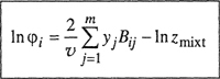
where the fugacity coefficient φ _i is defined by

(5-3)

and z is the compressibility factor of the mixture.

Equation (5-1) is used whenever the volumetric data are given in volume explicit form; i.e., whenever

(5-4)

Equation (5-2) is used in the more common case when the volumetric data are expressed in pressure-explicit form, i.e., whenever

(5-5)

The mathematical relation between volume, pressure, temperature, and composition is called the equation of state and most forms of the equation of state are pressure-explicit. Therefore, Eq. (5-2) is frequently more useful than Eq. (5-1). At low or moderate densities, it is often possible to describe volumetric properties of a gaseous mixture in a volume-explicit form; in that case Eq. (5-1) can be used. At high densities, however, volumetric properties are much better represented in pressure-explicit form, requiring the use of Eq. (5-2).

Equations (5-1) and (5-2) are exact and if the information needed to evaluate the integrals is at hand, then the fugacity coefficient can be calculated exactly. The problem of calculating fugacities in the gas phase, therefore, is equivalent to the problem of estimating volumetric properties. Techniques for estimating such properties must come not from thermodynamics, but rather from molecular physics; it is for this reason that Chap. 4, concerned with intermolecular forces, precedes Chap. 5.

5.1 The Lewis Fugacity Rule

A particularly simple and popular approximation for calculating fugacities in gas-phase mixtures is given by the Lewis rule; the thermodyaamic basis of the Lewis rule has already been given (Sec. 3.1). The assumption on which the rule rests states that at constant temperature and pressure, the molar volume of the mixture is a linear function of the mole fraction. This assumption (Amagat’s law) must hold not only at the pressure of interest but for all pressures up to the pressure of interest.

As shown in Sec. 3.1, the fugacity of component i in a gas mixture can be related to the fugacity of pure gaseous i at the same temperature and pressure by the exact relation

(5-6)

where is the partial molar volume, defined shortly after Eq. (3-14). According to Amagat’s law, = υ_i and assuming validity of this equality over the entire pressure range 0 → P the Lewis fugacity rale follows directly from Eq. (5-6):

(5-7)

or, in equivalent form,

(5-8)

where f_{pure i} and φ_{pure i} are evaluated for the pure gas at the same temperature and pressure as those of the mixture.

In effect, the Lewis rule assumes that at constant temperature and pressure, the fugacity coefficient of i is independent of the composition of the mixture and is independent of the nature of the other components in the mixture. These are drastic assumptions. On the basis of our knowledge of intermoiecular forces, we recognize that for component i deviations from ideal-gas behavior (as measured by φ_i) depend not only on temperature and pressure, but also on the relative amounts of component i and other components j, k,…; further, we recognize that φ_i must depend on the chemical nature of these other components that interact with component i. The Lewis rule, however, precludes such dependence; according to it, φ_i is a function only of temperature and pressure but not of composition.

Nevertheless, the Lewis rule is frequently used because of its simplicity for practical calculations. We may expect that the partial molar volume of a component i is close to the molar volume of pure i at the same temperature and pressure whenever the intermoiecular forces experienced by a molecule i in the mixture are similar to those that it experiences in the pure gaseous state. In more colloquial terms, a molecule i that feels “at home” while it is “with company”, possesses properties in the mixture close to those it has in the pure state. It therefore follows that for a component i, the Lewis fugacity rule is:

• Always a good approximation at sufficiently low pressures where the gas phase is nearly ideal.

• Always a good approximation at any pressure whenever i is present in large excess (say, y_i >0.9). The Lewis rule becomes exact in the limit as y_i→1.

• Often a fair approximation over a wide range of composition and pressure whenever the physical properties of all the components are nearly the same (e.g., nitrogen-carbon monoxide or benzene-toluene).

• Almost always a poor approximation at moderate and high pressures whenever the molecular properties of the other components are significantly different from those of i and when i is not present in excess. If y_i is small and the molecular properties of i differ much from those of the dominant component in the mixture, the error introduced by the Lewis rule may be extremely large (see Sec. 5.12).

One of the practical difficulties encountered in the use of the Lewis rule for vapor-liquid equilibria results from the frequent necessity of introducing a hypothetical state. At the temperature of the mixture, it often happens that P, the total pressure, exceeds , the saturation pressure of pure component i. In that case φ_{pure i}, the fugacity coefficient of pure gas i at the temperature and pressure of the mixture, is fictitious because pure gas i cannot physically exist at these conditions. Calculation of φ_{pure i} under such conditions requires assumptions about the nature of the hypothetical pure gas and consequently, further inaccuracies may result from use of the Lewis rule.

In summary, then, the Lewis fugacity rule is attractive because of convenience but it has no general validity. However, when applied in certain limiting situations, it frequently provides a good approximation.

5.2 The Virial Equation of State

As indicated at the beginning of this chapter, the problem of calculating fugacities for components in a gaseous mixture is equivalent to the problem of establishing a reliable equation of state for the mixture; once an equation of state exists, fugacities can be found by straightforward computation. Such computation presents no difficulties in principle although it may be tedious because it may require trial-arid-error calculations.

Many equations of state have been proposed and each year additional ones appear in the literature, but most of them are either totally or at least partially empirical. All empirical equations of state are based on more or less arbitrary assumptions that are not generally valid. Because the constants in an empirical equation of state for a pure gas have at best only approximate physical significance, it is difficult (and frequently impossible) to justify mixing rules for expressing the constants of the mixture in terms of the constants of the pure components that comprise the mixture. As a result, because mixing rules introduce further arbitrary assumptions, for typical empirical equations of state, one set of mixing rules may work well for one or several mixtures but poorly for others (Cullen and Kobe, 1955).

To calculate with confidence fugacities in a gas mixture, it is advantageous to use an equation of state where the parameters have physical significance, i.e. where the parameters can be related directly to intermolecular forces. One equation of state that possesses this desirable ability is the virial equation of state.

Figure 5-1 shows a plot of the compressibility factor as a function of density for helium, methane, and three binary mixtures containing 10, 25 and 50 rnole per cent water in methane. For these systems, the magnitudes of the intermolecular forces differ appreciably and depend strongly on density (or pressure). The compressibility factor for the methane mixture containing 10 mol % water deviates little from unity over a wide range of density, even when compared with the compressibility factors of pure methane or helium. However, as density increases, the compressibility factor plot for the same mixture shows a change in the slope from negative to positive. It is apparent that, to describe systems as those in Fig. 5-1, the parameters that appear in a gas-phase equation of state must account for a large variety of intermolecular forces that are responsible for the nonideaiity of the gas.

Figure 5-1 Compressibility factors for helium, methane and three water/methane mixtures as a function of density at 498.15 K (Joffrion and Eubank, 1988).

The virial equation of state for nonelectrolyte gases has a sound theoretical foundation, free of arbitrary assumptions (Mason and Spurling, 1969). The virial equation gives the compressibility factor as a power series in the reciprocal molar volume 1/ν;¹

¹ Equation (5-9) is frequently written in the equivalent form
                                               z = 1 + Bρ + Cρ² + Dρ³+…,
where p, the moiar density, is equal to l/υ. It is most conveniently derived using the grand partition function (see App. B) as, for example, in Hill (1986). The derivation shews that the virial equation is remarkably general, provided that the intermoleeuiar potential obeys certain well-defined restrictions.

(5-9)

In Eq. (5-9), B is the second virial coefficient, C is the third virial coefficient, D is the fourth, and so on. All virial coefficients are independent of pressure or density; for pure components, they are functions only of the temperature. The unique advantage of the virial equation follows, as shown later, because there is a theoretical relation between the virial coefficients and the intermolecular potential. Further, in a gaseous mixture, virial coefficients depend on composition in an exact and simple manner.

The compressibility factor is sometimes written as a power series in the pressure:

(5-10)

where coefficients B′, C′, D′,… depend on temperature but are independent of pressure or density. For mixtures, however, these coefficients depend on composition in a more complicated way than do those appearing in Eq. (5-9). Relations between the coefficients in Eq. (5-9) and those in Eq. (5-10) are derived in App.C with the results

(5-11)

(5-12)

(5-13)

Equation (5-9) is usually superior to Eq. (5-10) in the sense that when the series is truncated after the third term, the experimental data are reproduced by Eq. (5-9) over a wider range of densities (or pressures) than by Eq. (5-10), provided that the virial coefficients are evaluated as physically significant parameters. In that case, the second virial coefficient B is properly evaluated from low-pressure P-V-T data by the definition

(5-14)

Similarly, the third virial coefficient must also be evaluated from P-V-T data at low pressures; it is defined by

(5-15)

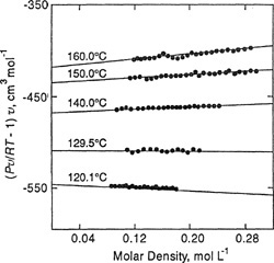
Reduction of P-V-T data to yield second and third virial coefficients is illustrated in Fig. 5-2, taken from the work of Douslin (1962) on methane. In addition to Douslin’s data, Fig. 5-2 also shows experimental results from several other investigalors. The coordinates of Fig. 5-2 follow from rewriting the virial equation in the form

(5-16)

Figure 5-2 Reduction of P-V-T data for methane to yield second and third virial coefficients (data from various sources).

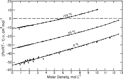
When isothermal data are plotted as shown, the intercept on the ordinate gives B, while C is found from the limiting slope as l/υ → 0. For mixtures, the same procedure is used, but in addition to isothermal conditions, each plot must also be at constant composition. An example is given in Fig. 5-3 for the mixture methanol/methyl acetate at several temperatures (Olf et al., 1989).

Figure 5-3 Reduction of P-V-Fdata for methanol/methyl acetate to yield second and third virial coefficients of approximateiy equimolar mixtures (Olf et al., 1989).

An illustration of the applicability of Eqs. (5-9) and (5-10) at two different temperatures is given in Figs. 5-4 and 5-5, based on Michels’ accurate volumetric data for argon (Michels et al., 1960; Guggenheim and McGlashan, 1960; Munn, 1964; Munn et al., 1965, 1965a). Using only low-pressure data along an isotherm, B and C were calculated as indicated by Eq. (5-16). These coefficients were then used to predict the compressibility factors at higher pressures (or densities). One prediction is based on Eq. (5-9) and the other on Eq. (5-10) together with Eqs. (5-11) and (5-12). Experimentally determined isotherms are also shown. In both cases, Eq. (5-9) is more successful than Eq. (5-10).²

² The comparisons shown in Figs. 5-4 and 5-5 are for the case where Eqs. (5-9) and (5-10) are truncated after the quadratic terms. When similar comparisons are made with these equations truncated after the linear terms, it often happens that, because of compensating errors, Eq. (5-10) provides a better approximation at higher densities than Eq. (5-9). See Chueh and Prausnitz (1967).

Figure 5-4 Compressibility factor for argon at -70°C

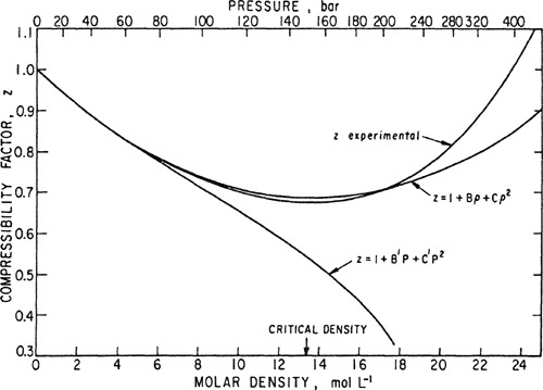
Figure 5-5 Compressibility factor for argon at -25°C

For many gases, it has been observed that Eq. (5-9), when truncated after the third term (i.e., when D and all higher virial coefficients are neglected), gives a good representation of the compressibility factor to about one half the critical density and a fair representation to nearly the critical density.

For higher densities, the virial equation is of little practical interest. Experimental as well as theoretical methods are not sufficiently developed to obtain useful quantitative results for fourth and higher virial coefficients. The virial equation is, however, applicable to moderate densities as commonly encountered in many typical vapor-liquid and vapor-solid equilibria.

The significance of the virial coefficients lies in their direct relation to intermolecular forces. In an ideal gas, the molecules exert no forces on one another. In the real world, no ideal gas exists, but when the mean distance between molecules becomes very large (low density), all gases tend to behave as ideal gases. This is not surprising because intermolecular forces diminish rapidly with increasing intermolecular distance and therefore forces between molecules at low density are weak. However, as density rises, molecules come into closer proximity with one another and, as a result, interact more frequently. The purpose of the virial coefficients is to take these interactions into account. The physical significance of the second virial coefficient is that it takes into account deviations from ideal behavior that result from interactions between two molecules. Similarly, the third virial coefficient takes into account deviations from ideal behavior that result from the interaction of three molecules. The physical significance of each higher virial coefficient follows in an analogous manner.

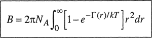
From statistical mechanics we can derive relations between virial coefficients and intermolecular potential functions (Hill, 1986). For simplicity, consider a gas composed of simple, spherically symmetric molecules such as methane or argon. The potential energy between two such molecules is designated by Γ(r), where r is the distance between molecular centers. The second and third virial coefficients are given as functions of Γ(r) and temperature by

(5-17)³

³ Similarly, the McMillan-Mayer solution theory provides the link between the osmotic second virial coefficient (B*₂₂) of a solute (see Sec. 4.11) dilute in a solvent medium and the potential of mean force, W₂₂:

where μ₃ is the chemical potential of the solvent. Osmotic third virial coefficients can also be calculated from the potential of mean force. While in a gas B depends only on temperature, in a dilute solution B*₂₂ depends on temperature and chemical potential of the solvent.

and

(5-18)

where f_ij ≡ exp(–Γ_ij/kT)–1, k is Boltzmann’s constant and N_A is Avogadro’s constant.⁴

⁴ Equation (5-18) assumes, for convenience, that the potential energy of molecules 1, 2, and 3 is given by the sum of the three binary potential energies (additivity assumption): Γ₁₂₃(r₁₂, r₁₃, r₂₃) = Γ₁₂(r₁₂) + Γ₁₃ (r₁₃) + Γ₂₃(r₂₃). This assumption is unfortunately not strictly correct, although in many cases, it provides a good approximation.

Similar expressions can be written for the fourth and higher virial coefficients. While Eqs. (5-17) and (5-18) refer to simple, spherically symmetric molecules, we do not imply that the virial equation is applicable only to such molecules; rather, it is valid for essentially all stable, uncharged (electrically neutral) molecules, polar or nonpolar, including those with complex molecular structure. However, in a complex molecule the intermolecular potential depends not only on the distance between molecular centers but also on the spatial geometry of the separate molecules and on their relative orientation. In such cases, it is possible to relate the virial coefficients to the intermolecular potential, but the mathematical expressions corresponding to Eqs. (5-17) and (5-18) are necessarily more complicated.

Special care must be taken with “reactive” molecules, for example, molecules like acetic acid that dimerize, as discussed in Sec. 5.9.

5.3 Extension to Mixtures

Perhaps the most important advantage of the virlal equation of state for application to phase equilibrium problems lies in its direct extension to mixtures. This extension requires no arbitrary assumptions. The composition dependences of all virial coefficients are given by a generalization of the statistical-mechanical derivation used to derive the virial equation for pure gases.

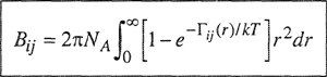
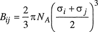
First, consider the second virial coefficient that takes into account interactions between two molecules. In a pure gas, the chemical identity of each of the interacting molecules is always the same; in a mixture, however, there are various types of two-molecule interactions depending on the number of components present. In a binary mixture containing species i and j, there are three types of two-molecule interactions, designated i-i, j-j, and i-j. For each of these interactions there is a corresponding second virial coefficient that depends on the intermolecular potential between the molecules under consideration. Thus B_ii is the second virial coefficient of pure i that depends on Γ_jj; B_jj is the second virial coefficient of pure; that depends on Γ_jj; and B_jj is the second virial coefficient corresponding to the i-j interaction as determined by Γ_ij, the potential energy between molecules i and j. If i and j are spherically symmetric molecules, B_ij is given by the same expression as that in Eq. (5-17):

(5-19)

The three second virial coefficients B_ii, B_jj, and B_ij are functions only of the temperature; they are independent of density (or pressure) and, what is most important, they are independent of composition. Because the second virial coefficient is concerned with interactions between two molecules, it can be rigorously shown that the second virial coefficient of a mixture is a quadratic function of the mole fractions y_i and y_j. For a binary mixture of components i and j,

(5-20)

For a mixture of m components, the second virial coefficient is given by a rigorous generalization of Eq. (5-20):

(5-21)

The third virial coefficient of a mixture is related to the various C_ijk coefficients that take into account interactions of three molecules i, j, and k; in a pure gas, the chemical identity of these three molecules is always the same but in a mixture, molecules i, j, and k may belong to different chemical species. In a binary mixture, for example, there are four C_ijk coefficients. Two of these correspond to the pure-component third virial coefficients and two of them are cross-coefficients. Because third virial coefficients take into account interactions of three molecules, it can be rigorously shown that the third virial coefficient of a mixture is a cubic function of the mole fractions. For a binary mixture of components i and j,

(5-22)

Equation (5-22) can be rigorously generalized for a mixture of m components:

(5-23)

Examining random-error propagation, Eubank and Hall (1990) found that there are optimum mixture compositions for calculation of cross-virial coefficients from binary gas-density experimental data. For determination of the cross-second virial coefficient B₁₂ from B_mixt using Eq. (5-20), the equimolar mixture is optimum as expected. However, to determine C₁₁₂ and C₁₂₂ from (at least) two density measurements of the mixture third virial coefficients using Eq. (5-22), it is best to use density data at mole fractions 0.25 and 0.75.

Coefficient C_ijk is related to intermolecular potentials Γ_ij, Γ_ik, and Γ_jk by an equation of the same form as that of Eq. (5-18):

(5-24)

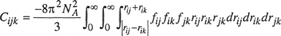
where f_ij ≡ exp(–Γ_ij/kT) – 1, f_ik ≡ exp(–Γ_ik/kT) –1, and f_jk ≡ exp(–Γ_jk/kT) –1.

The fourth, fifth, and higher virial coefficients of a gaseous mixture are related to the composition and to the various potential functions in an analogous manner: the nth virial coefficient of a mixture is a polynomial function of the mole fractions of degree n.

Equations (5-20) and (5-22) can be used to obtain, respectively, the second virial cross coefficients, B_ij, and the third virial cross coefficients, C_iij and C_ijj, from regression of the corresponding mixture virial coefficients.

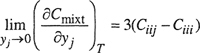
If experimental data are available for several compositions, the cross coefficients can be obtained from

(5-25)

and

(5-26)

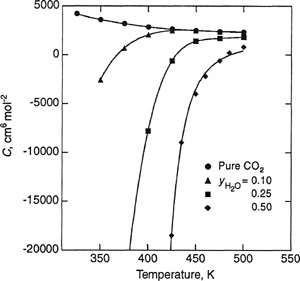
To illustrate, Figs. 5-6 and 5-7 show, respectively, experimental second and third virial coefficients for the carbon dioxide/water system as a function of temperature and mole fraction of water. As indicated in Fig. 5-7, uncertainties in estimating the limiting curvature makes it difficult to determine the third virial cross coefficients with high accuracy.

Figure 5-6 Experimental second virial coefficients for the CO₂/H₂O system as a function of the mole fraction of water, for various temperatures (Patel et al, 1987).

Figure 5-7 Experimental third virial coefficients for the CO₂/H₂O system as a function of temperature, for several mole fractions (Patel et al., 1987).

Equations (5-21) and (5-23) are rigorous results from statistical mechanics and are not subject to any assumptions other than those upon which the virial equation itself is based. The proof for these equations is not elementary and no attempt is made to reproduce it here. Such a proof may be found in advanced texts.⁵ However, the physical significance of Eqs. (5-21) and (5-23) is not difficult to understand because these equations are a logical consequence of the physical significance of the individual virial coefficients; each of the individual virial coefficients describes a particular interaction and the virial coefficient of the mixture is a summation of the individual virial coefficients, appropriately weighted with respect to composition.

⁵ See, for example, Hirschfelder et al. (1954), Hill (1986), or Mayer and Mayer (1977). It is shown in these, as well as in other references, that the nth virial coefficient is a polynomial in the mole fractions of degree n. These polynomial relations do not require the assumption of pairwise additivity of potential functions. That assumption is customarily used in evaluating the individual virial coefficients from potential functions but it is not required for establishing the composition dependence of the third (and higher) virial coefficients.

Extension of the virial equation to mixtures is based on theoretical rather than empirical grounds and it is this feature of the virial equation that makes it useful for phase-equilibrium problems. Empirical equations of state that contain constants having only empirical significance are useful for pure components but cannot be extended to mixtures without the use of somewhat arbitrary mixing rules for combining the constants. Extension of the virial equation to mixtures, however, follows in a simple and rigorous way from the theoretical nature of that equation.

5.4 Fugacities from the Virial Equation

Once we have decided on a relation that gives the volumetric properties of a mixture as a function of temperature, pressure, and composition, we can readily compute fugacities.

The virial equation for a mixture, truncated after the third term, is given by

(5-27)

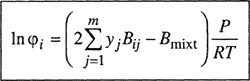
where z_mixt is the compressibility factor of the mixture, v is the molar volume of the mixture, and B_mixt and C_mixt are the virial coefficients of the mixture given by Eqs. (5-21) and (5-23). The fugacity coefficient for any component i in a mixture of m components is obtained by substitution in Eq. (3-53). When the indicated differentiations and integrations are performed, we obtain

(5-28)

In Eq. (5-28) the summations are over all components, including component i. For example, for component 1 in a binary mixture, Eq. (5-28) becomes

(5-29)

Similarly, for component 2,

(5-30)

Equation (5-28) is one of the most useful equations for phase-equilibrium thermodynamics. It relates the fugacity of a component in the vapor phase to its partial pressure through the theoretically-derived virial equation of state. The major practical limitation of Eq. (5-28) lies in its restriction to moderate densities. It may be applied to any component in a gas mixture regardless of whether or not that component can exist as a pure vapor at the temperature and pressure of the mixture; no hypothetical states are introduced. Further, Eq. (5-28) is not limited to binaries but is applicable without further assumptions to mixtures containing any number of components. Finally, Eq. (5-28) is valid for many types of (nonionized) molecules, polar and nonpolar, although it is unfortunately true that for practical purposes, theoretical calculation of the various B and C coefficients from statistical mechanics is restricted to relatively simple substances. However, this limitation is not due to failure of the virial equation or of the thermodynamic equations in Sec. 3.4; rather, it is a result of our present inability to describe adequately the intermolecular potential between molecules of complex structure.

Because data for second viriai coefficients⁶ are much more plentiful than those for third viriai coefficients, Eq. (5-28) is often truncated by omitting the quadratic term in density:

⁶ An extensive compilation of experimental virial coefficients is given by J. H. Dymond and E. B. Smith, 1980, The Virial Coefficients of Pure Gases and Mixtures, Oxford: Clarendon Press.

(5-31)

where z_mixt is given by

(5-32)

When the volume-explicit form of the virial equation [Eq. (5-10)] is used instead of the pressure-explicit form [Eq. (5-9)], and when terms in the third viriai coefficient C’ (and higher) are omitted, we obtain [using Eq. (5-11)]

(5-33)

Equation (5-33) is more convenient than Eq. (5-31) because it uses pressure, rather than volume, as the independent variable. Further, Eq. (5-33) is preferable because the assumption C’ = 0 often provides a better approximation than the assumption C = 0 in Eq. (5-31). However, both Eqs. (5-31) and (5-33) are valid only at low or moderate densities, approximately equal to but not exceeding (about) one-half the critical density.

In the limit as component i becomes infinitely dilute in component j, Eq. (5-31) for a binary mixture reduces to

Therefore, a reliable estimate of cross-coefficient B_ij is essential for the calculation of fugacity coefficients of dilute components.

5.5 Calculation of Virial Coefficients from Potential Functions

In previous sections we discussed the nature of the virial equation of state and, in Eq. (5-28), we indicated the way it may be used to calculate the fugacity of a component in a gaseous mixture. We must now consider how to calculate the virial coefficients that appear in Eq. (5-28) and, to do so, we make use of our discussion of intermolecular forces in Chap. 4.

First, we must recognize that the first term on the right-hand side of Eq. (5-28) is frequently much more important than the second term; at low or moderate densities, the second term is sufficiently small to allow us to neglect it. This is fortunate because we can estimate B’s with much more accuracy than we can estimate C’s.

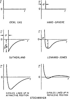
Equation (5-19) gives the relation between the second virial coefficient B_ij and the intermolecular potential function Γ_ij(r) for spherically symmetrical molecules i and j, where i and may, or may not, be chemically identical. If the potential function Γ_ij(r) is known, then B_ij can be calculated by integration as indicated by Eq. (5-19) and similarly, if the necessary potentials are known, C_ijk can be found from Eq. (5-24). Such integrations have been performed for many types of potential functions corresponding to different molecular models. A few models are illustrated in Figs. 5-8 and 5-9. We now give a brief discussion of each of them with reference to second virial coefficients, followed by a short section on third virial coefficients.

Ideal-Gas Potential. The simplest (trivial) case is to assume that Γ = 0 for all values of the intermolecular distance r. In that case, the second, third, and higher virial coefficients are zero for all temperatures and the virial equation reduces to the ideal-gas law.

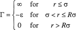
Hard-Sphere Potential. This model takes into account the nonzero size of the molecules but neglects attractive forces. It considers molecules to be like billiard balls; for hard-sphere molecules there are no forces between the molecules when their centers are separated by a distance larger than σ, the hard-sphere diameter, but the force of repulsion becomes infinitely large when they touch, at a separation equal to σ. The potential function Γ(r) is given by

(5-34)

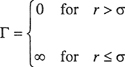
Substituting into Eqs. (5-19), we obtain for a pure component

(5-35)

Figure 5-8 Potential functions with zero, one, or two adjustable parameters.

For mixtures, the second virial coefficient B_ij (i≠j) is

(5-36)

The hard-sphere model gives a highly oversimplified picture of real molecules because, for a given gas, it predicts second virial coefficients that are independent of temperature. These results are in strong disagreement with experiment but give a rough approximation for the behavior of simple molecules at temperatures far above the critical. For example, helium or hydrogen have very small forces of attraction; near room temperature, where the kinetic energies of these molecules are much larger than their potential energies, the size of the molecules is the most significant factor that contributes to deviation from ideal-gas behavior. Therefore, at high-reduced temperatures, the hard-sphere model provides a reasonable but rough approximation. Because Eq. (5-34) requires only one characteristic constant, the hard-sphere model is a one-parameter model.

Figure 5-9 Potential functions with three adjustable parameters.

Sutherland Potential. According to London’s theory of dispersion forces, the potential energy of attraction varies inversely as the sixth power of the distance of separation. When this result is combined with the hard-sphere model, the potential function becomes

(5-37)

where K is a constant depending on the nature of the molecule. London’s equation [Eq. (4-19)] suggests that K is proportional to the ionization potential and to the square of the polarizability. The Sutherland model provides a large improvement over the hard-sphere model and it is reasonably successful in fitting experimental second-virialcoefficient data with its two adjustable parameters. Like the hard-sphere model, however, it predicts that at high temperatures the second virial coefficient approaches a constant value, although the best available data show that it goes through a weak maximum at a temperature very much higher than the critical. This limitation is not serious in typical phase-equilibrium problems where such high-reduced temperatures are almost never encountered except, perhaps, for helium.

Lennard-Jones’ Form of Mie’s Potential. As discussed in Chap. 4, Lennard-Jones’ form of Mie’s equation is

(5-38)

where ε is the depth of the energy well (minimum potential energy) and σ is the collision diameter, i.e., the separation where Γ = 0. Equation (5-38) gives what is probably the best known two-parameter potential for small, nonpolar molecules. In Lennard-Jones’ formula, the repulsive wall is not vertical but has a finite slope; this implies that if two molecules have very high kinetic energy, they may be able to interpenetrate to separations smaller than the collision diameter σ. Potential functions with this property are called soft-sphere potentials. The Lennard-Jones potential correctly predicts that, at a temperature very much larger than ε/k (k is Boltzmann’s constant), the second virial coefficient goes through a maximum. The temperature where B = 0 is called the Boyle temperature.

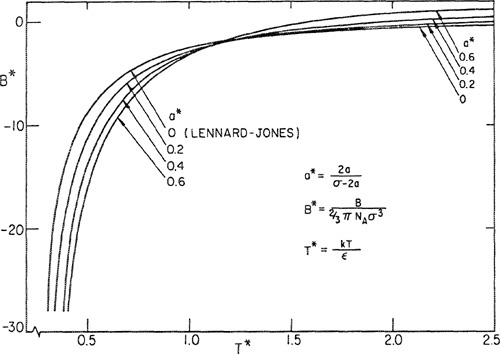
When Lennard-Jones’ potential is substituted into the statistical mechanical equation for the second virial coefficient [Eq. (5-17)], the required integration is not simple. However, numerical results have been obtained (Hirschfelder et al., 1954) as shown in Fig. 5-10, where the reduced (dimensionless) virial coefficient is a function of the reduced (dimensionless) temperature. The reducing parameter for the virial coefficient is proportional to collision diameter σ raised to the third power and that for the temperature is proportional to characteristic energy ε.

Figure 5-10 Second virial coefficients calculated from Lennard-Jones 6-12 potential

For many gases, second virial coefficients, as well as other thermodynamic and transport properties, have been interpreted and correlated successfully with the Len-nard-Jones potential. Unfortunately, however, it has frequently been observed that for a given gas, one set of parameters (ε and σ) is obtained from data reduction of one property (e.g., the second virial coefficient) while another set is obtained from data reduction of a different property (e.g., viscosity). If the Lennard-Jones potential were the true potential, then the parameters ε and σ should be the same for all properties of a given substance.

But even if attention is restricted to the second virial coefficient alone, there is good evidence that the Lennard-Jones potential is only an approximation, albeit a very good one in certain cases. It has been shown by Michels et al. (1958) that his highly accurate data for the second virial coefficient of argon over the temperature range -140 to +150°C cannot be fitted with the Lennard-Jones potential within the experimental error using only one set of parameters. This conclusion can be supported through a revealing series of calculations suggested by Michels et al. (1960). We take an experimental value of B corresponding to a certain temperature and then arbitrarily assume a value for ε. We now calculate the corresponding value of b₀ = (2/3)πN_Aσ³ that is required to force agreement between the experimental B and that calculated from the Lennard-Jones function. Next, we repeat the calculation at the same temperature assuming some other value of ε. In this way we obtain a curve on a plot of b₀ versus ε. We now perform the same series of calculations for another experimental value of B at a different temperature and again obtain a curve; where the two curves intersect should be the “true” value of ε and b₀. However, we find that when we repeat these calculations for several different temperatures, all the curves do not intersect at one point, as they should if the Lennard-Jones potential were exactly correct.

Such a plot is shown in Fig. 5-11; instead of a point of intersection, the curves define an area that gives a region rather than a unique set of potential parameters. Therefore, we conclude that even for a spherically symmetric, nonpolar molecule such as argon, the Lennard-Jones potential is not completely satisfactory (Guggenheim and McGlashan, 1960; Munn, 1964; Muan et al., 1965, 1965a). Such a conclusion, however, was reached only because Michels’ data are of unusually high accuracy and were measured over a large temperature range. For many practical calculations the Lennard-Jones potential is adequate. Lennard-Jones parameters for some fluids are given in Table 5-1.

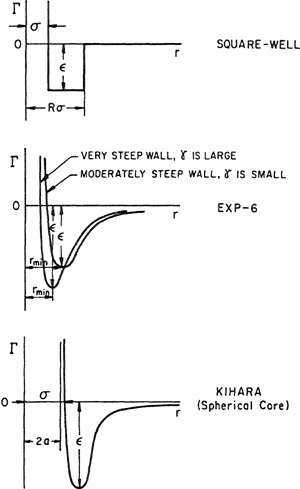
The Square-Well Potential. The Lennard-Jones potential is not a simple mathematical function. To simplify calculations, a crude potential was proposed having the general shape of the Lennard-Jones function. This crude potential is obviously an unrealistic simplification because it has discontinuities, but its mathematical simplicity and flexibility make it useful for practical calculations. The flexibility arises from the square-well potential’s three adjustable parameters: the collision diameter, σ; the well depth (minimum potential energy), ε; and the reduced well width, R. The square-well potential function is

Figure 5-11 Lennard-Jones’ parameters calculated from second-virial-coefficient data for argon. If perfect representation were given by Lennard-Jones’ potential, all isotherms would intersect at one point.

Table 5-1 Parameters for the Lennard-Jones potential obtained from second-virial coefficient data. ^§

^§ L. S. Tee, S. Gotoh, and W. E. Stewart, 1966, Ind. Eng. Chem. Fundam., 5: 356.

(5-39)

leading to

The square-well model has an infinitely steep repulsive wall and therefore, like the Sutherland model, it does not predict a maximum for the second virial coefficient. With its three adjustable parameters, good agreement can often be obtained between calculated and experimental second virial coefficients (Sherwood and Prausnitz, 1964).

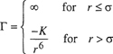
The Exp-6 Potential. A potential function for nonpolar molecules should contain an attractive term of the London type in addition to a repulsive term; little is known about that term but it must depend strongly on the intermolecular distance. For the repulsive term Mie, and later Leonard-Jones, used a term inversely proportional to r, the intermolecular distance, raised to a large power. Theoretical calculations, however, have suggested that the repulsive potential is not an inverse-power function but rather an exponential function of r. A potential function that uses an exponential form for repulsion and an inverse sixth power for attraction is called an exp-6 potential. (It is also sometimes referred to as a modified Buckingham potential.) This potential function contains three adjustable parameters and is written⁷

⁷ Equation (5-40) is valid only for r > s, where s (a very small distance) is that value for r where Γ goes through a (false) maximum. For completeness, therefore., it should be added that Γ = ∞ for r > s. The quantity s, however, is not an independent parameter and has no physical significance.

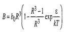
(5-40)

where -ε is the minimum potential energy at intermolecular separation r_min. The third parameter, γ, determines the steepness of the repulsive wall; in the limit, when γ = ∞, the exp-6 potential becomes the Sutherland potential that has a hard-sphere repulsive term.

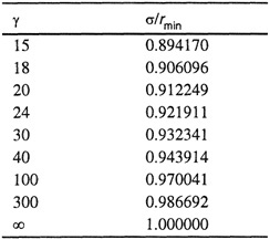
The collision diameter σ (i.e., the intermolecular distance where Γ = 0) is only slightly less than the distance r_min but the exact relation depends on the value of γ, as shown in Table 5-2. Numerical results for the second virial coefficient, based on Eq. (5-40), are available (Sherwood and Prausnitz, 1964a). Good agreement can often be obtained between calculated and observed second virial coefficients.

Table 5-2 Ratio σ/r_min for the exp-6 potential as a function of the repulsive steepness parameter γ.

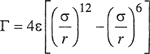
The Kihara Potential. According to Lennard-Jones’ potential, two molecules can interpenetrate completely provided that they have enough energy; according to this model, molecules consist of point centers surrounded by “soft” (i.e., penetrable) electron clouds. An alternative picture of molecules is to think of them as possessing impenetrable (hard) cores surrounded by penetrable (soft) electron clouds. This picture leads to a model proposed by Kihara. In crude mechanical terms, Kihara’s model (for spherically symmetric molecules) considers a molecule to be a hard billiard ball with a foam-rubber coat; a Lennard-Jones molecule, by contrast, is a soft ball made exclusively of foam rubber.

Kihara (1953, 1958, 1963) writes a potential function identical to that of Len-nard-Jones except that the intermolecular distance is taken not as that between molecular centers but rather as the distance between the surfaces of the molecules’ cores.⁸ For molecules with spherical cores, the Kihara potential is

⁸ When the cores are not spherical, the intermolecular distance is for the orientation that gives a minimum distance of separation.

(5-41)

where a is the radius of the spherical molecular core, ε is the depth of the energy well, and σ is the collision diameter, i.e., the distance r between molecular centers when Γ = 0.

Equation (5-41) is for the special case of a spherical core, but a more general form has been presented by Kihara for cores having other convex shapes such as rods, tetrahedra, triangles, prisms, etc. (Connolly and Kandakic, 1960; Prausnitz and Keeler, 1961; Prausnitz and Myers, 1963). Numerical results, based on Kihara’s potential, are available for second viriai coefficients for several core geometries and, in particular, for reduced (spherical) core sizes a*, where a* = 2a/(σ – 2a). When a* = 0, the results are identical to those obtained from Lennard-Jones’ potential. Because it is a three-parameter function, Kihara’s potential is successful in fitting thermodynamic data for a large number of nonpolar fluids, including some complex substances whose properties are represented poorly by the two-parameter Lennard-Jones potential. Figure 5-12 shows reduced second viriai coefficients calculated from Kihara’s potential.

Figure 5-12 Second viriai coefficients calculated from Kihara’s potential with a spherical core of radius a.

In our discussion of Lennard-Jones’ potential we indicated that Michels’ highly accurate second-virial-coefficient data for argon could not be represented over a large temperature range by the Lennard-Jones potential using only one set of potential parameters. However, these same data can be represented within the very small experimental error by the Kihara potential using only one set of parameters (Myers and Prausnitz, 1962; Rossi and Danon, 1966; O’Connell and Prausnitz, 1968). The ability of Kihara’s potential to do what Lennard-Jones’ potential cannot do is hardly surprising because the former potential has three adjustable parameters whereas the latter has only two. In fitting data for argon, the three Kihara parameters were determined by trial and error until the deviation between experimental and theoretical second viriai coefficients reached a minimum less than the experimental error. The magnitude of the core diameter obtained by this procedure is physically reasonable when compared to the diameter of the “impenetrable core” of argon as calculated from its electronic structure. Figure 5-13 shows results of a theoretical calculation of the electron density as a function of distance. While the results shown appear to justify confidence in the Kihara potential, the agreement indicated must not be considered “proof” of its validity. The “true” potential between two argon atoms is undoubtedly quite different from that given by Eq. (5-41) especially at very small separations. However, it appears that for practical calculation of common thermodynamic properties (except those at very high temperatures), Kihara’s potential is one of the most useful potential functions now available.

Figure 5-13 Charge distribution in argon (quoted by C. A. Coulson, 1962, Valence, 2^nd Ed. London: Oxford University Press).

One practical application of Kihara’s potential is for prediction of second virial coefficients at low temperatures where experimental data are scarce and difficult to obtain. To illustrate, Fig. 5-14 shows predicted and observed second virial coefficients for krypton at low temperatures; two sets of predictions were made, one with the Kihara potential and the other with the Lennard-Jones potential. In both cases potential parameters were obtained from experimental measurements made at room temperature and above. It is evident from Fig. 5-14 that even for such a “simple” substance as krypton, she Kihara potential is significantly superior to the Leonard-Jones potential. Kihara parameters for some fluids are given in Table 5-3.

Figure 5-14 Second virial coefficients for krypton. Predictions at low temperatures based on Lennard-Jones potential (a* = 0) and on Kihara potential.

Table 5-3 Parameters for the Kihara potential (spherical core) obtained from second-virial-coefficient data.§

For mixtures, Kihara’s potential gives B_ij(i ≠ j) when the pure-component core parameters and the unlike-pair potential parameters ε_ij and σ_ij are specified. The latter two are frequently related to the pure-component parameters by empirical combining rales. However, the core parameter for the i-j interaction can be derived exactly from the core parameters for the i-i and j-j interactions even for nonspherical cores (Kihara, 1953, 1958, 1963; Myers and Prausnitz, 1962).

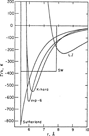
The difficulty of determining “true” intermolecular potentials from second virialcoefficient data is illustrated in Figs. 5-15 and 5-16 that show several potential functions for argon and for neopentane. Each of these functions gives a good prediction of the second virial coefficient; the three-parameter potentials give somewhat better predictions than the two-parameter potentials, but all of them are in fairly good agreement with experiment. However, the various potential functions differ very much from one another, especially for neopentane.

Figures 5-15 and 5-16 give striking evidence that agreement between a particular set of experimental results and those calculated from a particular model should not be regarded as proof that the model is correct.⁹ Models are useful in molecular thermodynamics but one must not confuse utility with truth. Figures 5-15 and 5-16 provide a powerful illustration of A. N. Whitehead’s advice to scientists: “Seek simplicity but distrust it”.

⁹ A more nearly “true” potential can be obtained by simultaneous analysis of experimental data for a variety of properties: second virial coefficients, gas-phase viscosity, diffusivity, and thermal diffusivity. Such analysis has produced a “best” potential function for argon. See Dymond and Alder (1969) and Barker and Pompe (1968).

Figure 5-15 Potential functions for argon as determined from second-virial-coefficient data.

The Stockmayer Potential. All of the potential functions previously described are applicable only to nonpolar molecules. We now briefly consider molecules that have a permanent dipole moment; for such molecules Stockmayer proposed a potential that adds to the Lennard-Jones formula for nonpolar forces an additional term for the potential energy due to dipole-dipole interactions. Dipole-induced dipole interactions are not considered explicitly although it may be argued that because these forces, like London forces, are proportional to the inverse sixth power of the intermolecular separation, they are, in effect, included in the attractive term of the Lennard-Jones formula. For polar molecules, the potential energy is a function not only of intermolecular separation but also of relative orientation. Stockmayer’s potential is

Figure 5-16 Potential functions for neopentane as determined from second-viriai-coefficient data.

(5-42)

where F_θ is a known function of the angles θ₁, θ₂, and θ₃ that determine the relative orientation of the two dipoles [see Eq. (4-7)]. This potential function contains only two adjustable parameters because the dipole moment μ is an independently determined physical constant.

The collision diameter σ in Eq. (5-42) is the intermolecular distance where the potential energy due to forces other than dipole-dipole forces becomes equal to zero.

Numerical results, based on Stockmayer’s potential, are available for the second virial coefficient (Rowlinson, 1949). Figure 5-17 shows reduced second virial coefficients calculated from Stockmayer’s potential as a function of reduced temperature and reduced dipole moment. The top curve (zero dipole moment) is for nonpolar Lennard-Jones molecules and it is evident that the effect of polarity is to lower (algebraically) the second virial coefficient due to increased forces of attraction, especially at low temperatures, as suggested by Keesom’s formula (see Sec. 4.2). Stockmayer’s potential has been used successfully to fit experimental second-virial-coefficient data for a variety of polar molecules; Table 5-4 gives parameters for some polar fluids and Table 5-5 shows some illustrative results for trifluoromethane.

Figure 5-17 Second viriai coefficients calculated from Stockmayer’s potential for polar molecules.

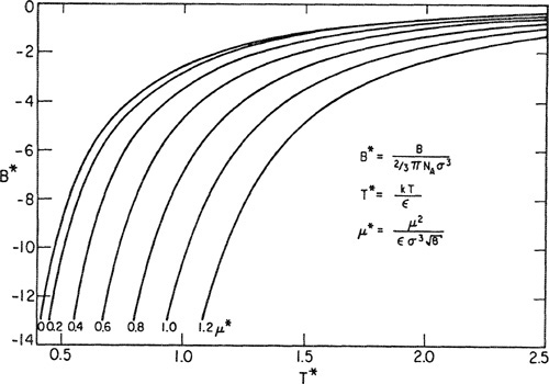
Table 5-4 Parameters for Sockmayer’s potential for poiar fluids.^*

^* R. F. Blanks and J. M. Prausnitz, 1962, AIChEJ., 8: 86.

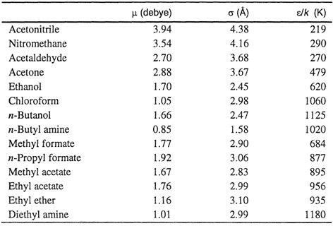
Table 5-5 Second virial coefficients of trifiuoromethane. Calculated values from Stockmayer potential with ε/k = 188 K, σ = 4.83 Å, and μ = 1.65 debye.

The various potential models discussed above may be used to calculate B_ij as well as B_ii. The calculations for B_ij are exactly the same as those for B_ij when potential Γ_ij is used rather than potential Γ_ii. In the Stockmayer potential, when i ≠ j, the reduced dipole moment μ* in Fig. (5-17) becomes .

5.6 Third Virial Coefficients

In the preceding section, attention was directed to the second virial coefficient. We now consider briefly our limited knowledge concerning third virial coefficients.

Equations (5-18) and (5-24) give expressions for the third virial coefficient in terms of three two-body intermolecular potentials. In the derivation of these equations, an important simplifying assumption was made; i.e., we assumed pairwise additivity of potentials. The third virial coefficient takes into account deviations from ideal-gas behavior due to three-molecule interactions; for a collision of three molecules i, j, and k, we need Γ_ijk the potential energy of the three-molecule assembly. However, in the derivation of Eqs. (5-18) and (5-24) it was assumed that

(5-43)

Equation (5-43) says that the potential energy of the three molecules i, j, and k is equal to the sum of the potential energies of the three pairs i-j, i-k, and j-k. This assumption of pairwise additivity of intermolecular potentials is a common one in molecular physics because little is known about three-, four- (or higher) body forces. For an m- body assembly, the additivity assumption takes the form

(5-44)

We also used this assumption in Sec. 4.5, where we briefly considered some properties of the condensed state. While there is no rigorous proof, it may well be that because of cancellation effects, the assumption of pairwise additivity becomes better as the number of particles increases. However, it is likely that the assumption is somewhat in error for a three-body assembly (Rowlinson, 1965). Therefore, calculations for the third virial coefficient using Eq. (5-18) must be considered as approximations.

For any realistic potential, the calculation of third virial coefficients is complicated and, to obtain numerical results, we require a computer. Numerical computations have been carried out for several potential functions and results for pure nonpolar components are available (Sherwood and Prausnitz, 1964a; Kihara, 1953, 1958, 1963; Graben and Present, 1962; Sherwood et al, 1966). For example, Fig. 5-18 gives reduced third virial coefficients as calculated from Kihara’s potential. In these calculations, a spherical core was used and pairwise additivity was assumed. The reduced third virial coefficient, reduced temperature, and reduced core are defined by

Figure 5-18 Third virial coefficient from Kihara potential assuming pairwise additivity.

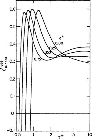
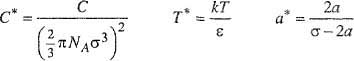
where -ε is the minimum energy in the potential function, σ is the intermolecular distance when the potential is zero, and a is the core radius. For a* = 0, the results shown are those obtained from Lennard-Jones’ potential

Some efforts have been made to include nonadditivity corrections in the calculation of third virial coefficients (Sherwood and Prausnitz, 1964a; Kihara, 1953, 1958, 1963). These corrections are based on a quantum-mechanical relation derived by Axilrod and Teller (1943) for the potential of three spherical, nonpolar molecules at separations where London dispersion forces dominate. The nonadditive correction is a function of the polarizability and at lower temperatures it is large; its overall effect is that it approximately doubles the calculated third virial coefficient at its maximum, steepens the slope near the peak value and shifts the maximum to a lower reduced temperature.

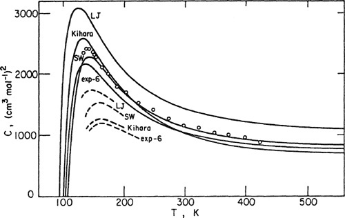
Calculated and observed third virial coefficients for argon are shown in Fig. 5-19. Calculated results are based on four potential functions; for each of these, the parameters were determined from second-virial-coefficient data. The solid lines include the nonadditivity correction but the dashed lines do not; it is clear that the nonadditivity correction is appreciable.

Figure 5-19 Calculated and observed third virial coefficients for argon. Solid lines include Axilrod-Teller nonadditivity corrections. Dashed Sines show a portion of calculated results assuming additivity. Circles represent experimental data of Michels (1958).

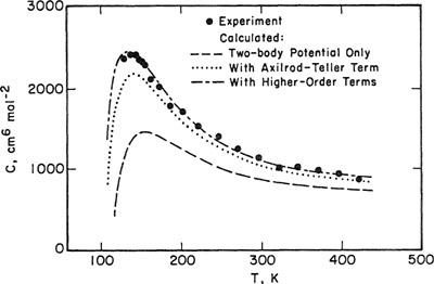
Barker and Henderson (1976) have presented a definitive study of the third virial coefficient of argon; their results are shown in Fig. 5-20. The lowest line shows calculations based on the assumption of pairwise additivity as given by Eq. (5-43). For the two-body potential for argon, Barker and Henderson used an expression obtained from data reduction using two-body experimental information: second virial coefficients and gas-phase transport properties at low densities. The middle line shows calculations based on a three-body potential (Γ_ijk) that includes first-order corrections to the additivity assumption. (This correction is called the Axilrod-Teller correction.) The top line shows calculations that include second- and third-order corrections. These calculations agree with experiment within experimental error.

Without going into details, we can indicate the nature of the three-body corrections. First, we recall that in London’s theory of dispersion forces, the potential is approximated by a series; for a two-body potential it has the form

(5-45)

where r is the center-to-center distance between two molecules. The leading coefficient is

(5-46)

where α is the polarizability, I is the ionization potential, and ε₀ is the vacuum permittivity. Coefficients C₈ and C₁₀ (not reproduced here) give the higher-order terms in London’s potential. (In many practical calculations these terms are ignored.)

For a three-body potential, the first-order correction to the additivity assumption is obtained from London’s theory, restricting attention to the leading (C₆/r⁶) term. This first-order (Axilrod-Teller) correction to Γ_ijk is

(5-47)

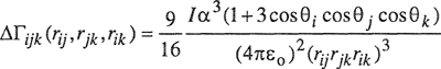
where θ_i, θ_j, and θ_k are the three angles of a triangle whose sides are r_ij, r_jk, and r_ik.

Second-order corrections for nonadditivity are based on London’s theory, restricting attention to the first two terms in the series; third-order corrections for nonad ditivity are based on London’s theory, restricting attention to the first three terms in the series. Still higher corrections appear to be negligible.

The important difference between Barker and Henderson’s results (Fig. 5-20) and those of earlier workers (Fig. 5-19) lies in the two-body potential. The earlier work is based on a two-body potential that follows only from second virial-coefficient data and, as suggested by Fig. 5-15, these data alone do not yield a unique potential function. However, Barker and Henderson were able to use a unique two-body potential obtained from other dilute-gas data in addition to second-virial-coefficient data. The excellent agreement between theory and experiment, shown in Fig. 5-20, follows from an excellent two-body potential.

Figure 5-20 Third virial coefficients for argon (Barker and Henderson, 1976).

Due to experimental difficulties, there are few reliable values of third virial coefficients. It is therefore not possible to make a truly meaningful comparison between calculated and observed third virial coefficients; not only are experimental data not plentiful, but frequently they are of low accuracy. Ever, when calculated from very good P-V-T data, the accuracy of third virial coefficients is about one order of magnitude lower than that for second virial coefficients. To the extent that a comparison could be made, Sherwood (1964) found that the Lennard-Jones potential (with nonadditivity correction) generally predicted third virial coefficients that were too high, especially for larger molecules (such as pentane or benzene) where the predictions were very poor. The three-parameter potentials (square-well, exp-6, and Kihara) gave much better predictions; however, in view of the uncertainties in the data, and because corrections for nonadditive repulsive forces have been neglected, it is not possible to give a quantitative estimate of agreement between theory and experiment.

Little work has been done on the third virial coefficient of mixtures. The cross-coefficients, assuming additivity, can be calculated by Eq. (5-24) and the nonadditivity correction to these cross-coefficients, based on the formula of Axilrod and Teller, can also be computed as shown by Kihara (1953, 1958, 1963). However, the results of such calculations cannot be presented in a general manner; the coefficient C_ijk (for i≠j≠k) is a function of five independent variables for a two-parameter potential; for a three-parameter potential, eight independent variables must be specified.

An approximate method for calculating Cp was proposed by Orentlicher (1967), who showed that, subject to several simplifying assumptions, a reasonable estimate of C_ijk can be made based on Sherwood’s numerical results for the third virial coefficient of pure gases.¹⁰ Component i is chosen as a reference component; let C_ii(T) stand for the third virial coefficient of pure i at the temperature T of interest. Let the potential function between molecules i and j be characterized by the collision diameter σ_ij and the energy parameter ε_ij. Similarly, the potential function for the i-k pair is characterized by σ_ik and ε_ik and that for the j-k pair by σ_jk and ε_jk Orentlicher’s approximation is

¹⁰ Orentlicher’s approximation has been critically discussed by D. E. Siogryn, 1968, J. Chern. Phys., 48: 4474,

(5-48)

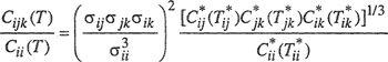
where T_ij^* = kT/ε_ij etc., and where the individual reduced coefficients C_ij^* etc., are obtained from available tables for pure components using any one of several popular potential functions.¹¹ Orentlicher’s formula appears to give good results for mixtures where the components do not differ much in molecular size and characteristic energy. The accuracy of the approximation is difficult to assess, but it is probably useful for mixtures at those temperatures where the third virial coefficient of each component has already passed its maximum. Table 5-6 gives some observed and calculated third-virial cross coefficients for binary mixtures. Because the uncertainty in the experimental results is probably at least ±100 (cm³ mol^-1)², agreement between calculated and experimental results is good for these particular mixtures.

¹¹ C_j^* is a function of KT/ε_ij and, perhaps, of some additional parameter such as a_ij^*, for the Kihara potential. This function, however, is the same as that for C_ii^*, that in turn depends on KT/ε_ii and, perhaps, on a_ii^*

Table 5-6 Experimental and catenated third-virial cross coefficients for some binary mixtures (OrentSicher, 1967).

Third virial coefficients for polar gases were calculated by Rowlinson (1951) using the Stockmayer potential and assuming additivity. Because experimental data are scarce and of low accuracy, it is difficult to make a meaningful comparison between calculated and experimental results.

5.7 Virial Coefficients from Corresponding-States Correlations

Because there is a direct relation between virial coefficients and interraolecular potential, it follows from the molecular theory of corresponding states (Sec. 4.12) that virial coefficients can be correlated by data reduction with characteristic parameters such as critical constants. A few correlations are given in the following paragraphs.

The major part of this section is concerned with second virial coefficients for nonpolar gases. We cannot say much about third virial coefficients because of the scarcity of good experimental data and because of the nonadditivity problem mentioned in the preceding section. Further, our understanding of polar gases is not nearly as good as that of nonpolar gases, because again, good experimental data are not plentiful for polar gases, and because theoretical models, based on ideal dipoles, often provide poor approximations to the behavior of real polar molecules.

Equation (5-17) relates second virial coefficient B to intermolecular potential Γ. Following the procedure given in Sec. 4.12, we assume that the potential Γ can be written in dimensionless form by

(5-49)

where ε is a characteristic energy parameter, CT is a characteristic size parameter, and F is a universal function of the reduced intermoiecular separation. Upon substitution, Eq. (5-17) can then be rewritten in dimensionless form:

(5-50)

If we set σ³ proportional to critical volume υ_c’ and ε/k proportional to critical temperature T_c’ we obtain an equation of the form

(5-51)

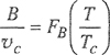
where F_B is a universal function of reduced temperature.

Equation (5-51) says that the reduced secoad virial coefficient is a generalized function of reduced temperature; this function can either he determined by specifying the universal potential function Γ/ε and integrating, as shown by Eq. (5-50), or by a direct correlation of experimental data for second virial coefficients.

For example, McGlashan and Potter (1962) plotted on reduced coordinates experimentally determined second virial coefficients for methane, argon, krypton, and xenon; the data for these four gases were well correlated by the empirical equation

(5-52)

Equation (5-52) was established from pure-component data but, utilizing the results of statistical mechanics and the molecular theory of corresponding states, it is readily extended to mixtures. To find B for a pure component, we use critical constants υ_c and T_c for that component; for a mixture of m components we first recall that the second virial coefficient is a quadratic function of the mole fraction [Eq. (5-21)]:

(5-53)

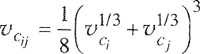
To calculate cross-coefficient B_ij (i≠j) we again use Eq. (5-52), but we must now specify parameters υ_ij and T_cij If we use the common, semiempirical combining rules for the characteristic parameters of the potential function Γ_ij, i.e.,

(5-54)

and

(5-55)

it then follows from our previous assumptions that

(5-56)

and

(5-57)

The geometric-mean approximation for T_c12 expressed by the above equation appears to be an upper limit; for asymmetric systems (i.e., mixtures whose components differ appreciably in molecular size), T_c12 is usually smaller than the geometric mean of T_c1, and T_c2. Subject to several simplifying assumptions, it can be shown from London’s dispersion formula (Sec. 4.4) that

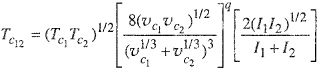
where I is the ionization potential and q is a positive exponent. Each of the bracketed quantities is equal to or less than unity and therefore the geometric mean for T_C12 [Eq. (5-57)] represents an upper limit. While the London formula is useful for showing that the geometric mean for T_C12 is a maximum, it is usually not reliable for a quantitative correction of the geometric-mean assumption.

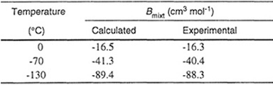
To illustrate the applicability of Eq. (5-52) for a mixture, let us make the reasonable assumption that this equation holds also for nitrogen; we can then calculate the second virial coefficient of a mixture of argon and nitrogen using only the critical volume and critical temperature for each of these pure components. Table 5-7 shows results obtained at three temperatures for an equimolar mixture argon/nitrogen using Eqs. (5-52), (5-53), (5-56), and (5-57). Calculated results are in excellent agreement with those found experimentally by Grain and Sonntag (1965).

Table 5-7 Experimental and calculated second virial coefficients for an equimolar mixture of argon/nitrogen.

Equation (5-52) gives a good representation of the second virial coefficients of small, nonpolar molecules but for larger molecules Eq. (5-52) is no longer satisfactory. For example, McGlashan et al. (1962, 1964} measured second virial coefficients for normal alkanes and α-olefins containing up to eight carbon atoms; to represent their own data, as well as those of others, they used an amended form of Eq. (5-52), i.e.,

(5-58)

where n stands for the number of carbon atoms.¹² Clearly, for methane (n = 1) Eq. (5-58) reduces to Eq. (5-52). Because experimental critical volumes for α-olefins are not highly accurate and because critical volumes for α-olefins have not been measured for n > 4, McGlashan et al., suggest that for these fluids the critical volumes be calculated from the expression

¹² McGlashan and Potter’s correlation applies equally well for some polymethyl compounds (e.g., tetramethylsilane, 2-methylbutane) taking the characteristic parameter n to be the number of methyl groups (J. M. Barbarin-Castillo and I. A. McLure, 1993, J. Chern. Thermodynamics, 25: 1521).

(5-59)

Equation (5-58) is plotted in Fig. 5-21 to illustrate the importance of the third parameter, n, especially at low reduced temperatures. The experimental data for hydrocarbons of different chain length clearly show the need for a third parameter in a corresponding-states correlation. This need indicates that a potential function containing only two characteristic constants is not sufficient for describing the thermodynamic properties of a series of compounds that, although chemically similar, differ appreciably in molecular size and shape.

Figure 5-21 Corresponding-states correlation of McGlashan for second virial coefficients of normal paraffins and α-olefins.

While the addition of a third parameter significantly improves the accuracy of a corresponding-states correlation for the second virial coefficients of pure fluids, it unfortunately introduces the need for an additional combining rule when applied to the second virial coefficients of mixtures. Suppose, for example, that we want to use Eq. (5-58) for predicting the second virial coefficient of a mixture of propene and α-heptene. Let 1 stand for propene and 2 for heptene; how shall we compute the cross-coefficient B₁₂? For the characteristic volume and temperature we have the (at best) semitheoretical combining rules given by Eqs. (5-56) and (5-57). We must also decide on a value of n₁₂ and, because B₁₂ refers to the interaction of one propene molecule with one heptene molecule, we are led to the rule

(5-60)

that, in this case, gives n₁₂ = 5. While this procedure appears reasonable, we must recoganize that Eq. (5-60) has little theoretical basis; it is strictly an ad hoc, phenomenological equation that, ultimately, can be justified only empirically. McGlashan et al. measured volumetric properties of a nearly equimolar mixture of propene and heptene. The second virial coefficients of the mixture at several temperatures are shown in Fig. 5-22. Calculated results were obtained from Eq. (5-53); individual coefficients B₁₁, B₂₂, and B₁₂ were determined from Eq. (5-58) and from the combining Miles given by Eqs. (5-56), (5-57), and (5-60). In this system, agreement between calculated and experimental results is excellent; good agreement was also found for mixtures of propane and heptane and for mixtures of propane and octane (McGlashan and potter, 1962).

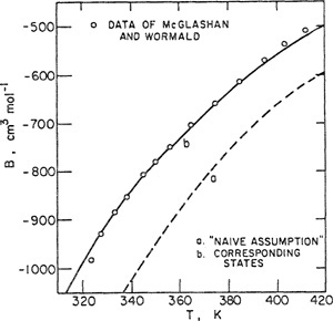
Figure 5-22 Second virial coefficients of a mixture containing 50.05 mote percent propene and 49, 95 mole percent α-heptene.

For comparison, Fig. 5-22 also shows results calculated with the attractively simple assumption

(5-61)

Guggenheim¹³ appropriately calls Eq. (5-61) the “naive assumption”. It can readily be shown that Eq. (5-61) follows from Amagat’s law (or the Lewis rale); when Eq. (5-61) is substituted into the exact Eq. (5-53), we obtain the simple but erroneous result

¹³ E. A. Guggenheim, 1952, Mixtures, Oxford: Clarendon Press.

(5-62)

Figure 5-22 shows that Eq. (5-62) is in significant disagreement with experimental data.

The Pitzer-Tsonopoulos Correlation. In Sees. 4.12 and 4.13 we pointed out that the applicability of corresponding-states correlations could be much extended if we distinguish between different classes of fluids and characterize these classes with an appropriate, experimentally accessible parameter. With this extension, the theory of corresponding states is applied separately to any one class containing a limited number of fluids rather than to a very large number of fluids belonging to different classes.

The classifying parameter suggested by Pitzer is w, the acentric factor, a macroscopic measure of how much the force field around a molecule deviates from spherical symmetry. The acentric factor is (essentially) zero for spherical, nonpolar molecules such as the heavy noble gases and for small, highly symmetric molecules such as methane. The definition of ω was given earlier [Eq. (4-86)]; it is

(5-63)

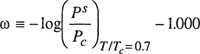
where P^s is the saturation (vapor) pressure and P_c is the critical pressure. Some acentric factors are given in Table 4-14. Other classifying parameters have been proposed (Meissner and Seferian, 1951; Riedel, 1956; Rowlinson, 1955) but the acentric factor is the most practical because it is easily evaluated from experimental data that are both readily available and reasonably accurate for most common substances.

When applied to the second virial coefficient, the extended theory of corresponding states asserts that for all fluids in the same class,

(5-64)

where, as before, σ is a characteristic molecular size and ε/k is a characteristic energy expressed in units of temperature. Function F_ω depends on the acentric factor ω and, for any given ω, it applies to all substances having that ω.

Upon replacing σ and ε/k with macroscopic parameters, Eq.(5-64) becomes

(5-65)¹⁴

¹⁴ Corresponding states sets σ³ proportional to υ_c But υ_c = z_c RT_C IP_C In Eq. (5-65), because z_c is a function only of ω, z_c has been absorbed in F_ω. By contrast, z_c appears explicitly in Eq. (5-66).

Schreiber and Pitzer (1989) have proposed a correlation of the form indicated by Eq. (5-65). They write

(5-66)

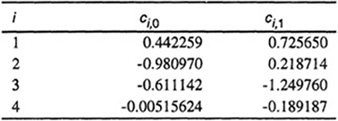
Here, T_R = T/T_C is the reduced temperature and z_c is the compressibility factor at ihe critical point approximated by z_c = 0.291-0.08ω. Coefficients C₁, c₂, c₃, and c₄ depend on acentric factor according to

(5-67)

Table 5-8 gives coefficients c_i,0 and C_i,1, determined from a large body of experimental data for nonpolar or slightly polar fluids. Highly polar fluids such as water, nitriles, ammonia, and alcohols were not included; also, the quantum gases helium, hydrogen and neon were omitted.

Table 5-8 Coefficients for Eq. (5-67).

Tsonopoulos (1974, 1975, 1978) gave another correlation for second virial coefficients in the form

(5-68)

where

(5-69)

(5-70)

Figure 5-23 shows the reduced second virial coefficient as a function of reciprocal reduced temperature for three ω. It is clear that the introduction of a third parameter has a pronounced effect, especially at low reduced temperatures.

Figure 5-23 Reduced second virial coefficients.

Equations (5-68), (5-69), and (5-70) [and other similar equations like those given by Mak and Lielmezs (1989)] provide a good correlation for the second virial coefficients of normal fluids. A normal fluid is one whose molecules are of moderate size, are nonpolar or else slightly polar, and do not associate strongly (e.g., by hydrogen bonding); further, it is a fluid whose configurational properties can be evaluated to a sufficiently good approximation by classical, rather than quantum statistical mechanics. For the three quantum gases, helium, hydrogen, and neon, good experimental results are available (see App. C), and therefore there is no need to use a generalized correlation for calculating the second virial coefficients of these gases. However, effective critical constants for quantum gases are useful for calculating properties of mixtures that contain quantum fluids in addition to normal fluids, as discussed later.

For polar and hydrogen-bonded fluids, Tsonopoulos suggested that Eq. (5-68) be amended to read¹⁵

¹⁵ Similar equations were proposed by Hayden and O’Connell (1975) and by Tarakad and Daneer (1977).

(5-71)

where

(5-72)

Constants a and b cannot easily be generalized, but for polar fluids that do not hydrogen-bond, Tsonopoulos found that b = 0.

Figure 5-24 shows constant a as a function of reduced dipole moment for a variety of non-hydrogen-bonded polar fluids. The equations given in the same figure present a compromise best fit for the polar fluids indicated.

Figure 5-24 Correlating constant a for some polar fluids. Top curve for ketones, aldehydes, alkyl nitriles, ethers, and carboxylic acid esters; lower curve for alkyl halides, mercaptans, sulfides, and disulfides.

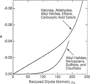
As shown in Fig. 5-24, Tsonopoulos (1990) suggests separate equations, one for each group of different chemical species. The top curve in Fig. 5.24 is recommended for ketones, aldehydes, alkyl nitriles, ethers, and carboxylic-acid esters,

(5-73)

However, for alkyl halides, mercaptans, sulfides, and disulfides, the bottom curve of Fig. 5-24 should be used:

(5-74)

In Eqs. (5-73) and (5-74), µ_R is the reduced dipole moment defined by where the units are debye for the dipole moment µ, bar for P_c, and kelvin for T_c.

(5-75)

As Fig. 5-24 shows, Eqs. (5-73) and (5-74) approach closely at high µ_R suggesting a unique relation between a and µ_R for strongly polar, non-dimerizing organic compounds.

For water the recommended a is -0.0109.

It is difficult to correlate second virial coefficients of polar and hydrogen-bonded fluids because we do not adequately understand the pertinent intermolecular forces and also because reliable experimental second-virial-coefficient data for such fluids are relatively scarce. For strongly hydrogen-bonded fluids, the virial equation is not useful for describing vapor-phase imperfections. For such fluids a chemical theory (dimerization) is required, as discussed in Sec. 5.8.

Third Virial Coefficients. Reliable experimental data are rare for third virial coefficients of pure gases, and good third virial coefficients for gaseous mixtures are extremely rare. In addition to the scarcity of good experimental results, it is difficult to establish an accurate corresponding-states correlation because, as briefly discussed earlier (Secs. 5.2 and 5.6), third virial coefficients do not exactly satisfy the assumption of pairwise additivity of intermolecular potentials. Fortunately, however, as shown by Sherwood (1966), nonadditivity contributions to the third virial coefficient from the repulsive part of the potential tend to cancel, at least in part, nonadditivity contributions from the attractive part of the potential; further, these contributions appear to be a function primarily of the reduced polarizability and they are important only in part of the reduced temperature range, at temperatures near or below the critical temperature.

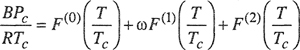
Several corresponding-states correlations are available for the third virial coefficients of gases and gas mixtures. Those of Chueh and Prausnitz (1967), Pope et al. (1973), De Santis and Grande (1979), and Orbey and Vera (1983) are suitable for nonpolar gases, whereas the correlation presented by Besher and Lielmezs (1992) also provides estimates for polar fluids. Typically these correlations give the reduced third virial coefficient through the generalized correlation,

(5-76)

where F⁽⁰⁾ and F⁽¹⁾ are regressed from experimental data.

For polar compounds, Besher and Lielmezs suggested that the above equation should take the form

(5-77)

where µ_R is the reduced dipole moment [defined by Eq. (5-75)] and x is an empirical, substance-dependent constant.

For the correlation of Orbey and Vera, functions F⁽⁰⁾ and F⁽¹⁾ in Eq. (5-76) are given by

(5-78)

(5-79)

Figure 5-25 compares experimental with calculated third virial coefficients for (nonpolar) sulfur hexafluoride obtained from the correlations of De Santis and Grande, Orbey and Vera, and Besher and Lielmezs. As Fig. 5-25 shows, all three methods compare well with experiment.

Figure 5-25 Reduced third virial coefficient of sulfur hexafluoride as a function of reduced temperature. Experiment: (from various sources). Calculated:…… De Santis and Grande (1979);…. Orbey and Vera (1983); — Besher and Lieimezs (1992).

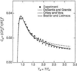
For mixtures, it is difficult to predict the cross-coefficients C_ijk. Studies by Stogryn (1968, 1969, 1970) indicate that no simple approximation procedure is entirely satisfactory; however, the approximation suggested by Orentlicher is useful [see Eq. (5-48)]. In its simplest form, Orentlicher’s approximation suggests that

(5-80)

Coefficient C_ij is the third virial coefficient for a hypothetical pure gas whose potential-energy function is characterized by distance parameter σ_ij and energy parameter ε_ij or, in corresponding-states terms,

(5-81)

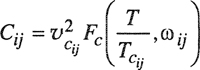
where F_c is the correlating equation for the third virial coefficient of a pure fluid.

A simple combining rule [e.g., Eq. (5-56)] is used for v_cij, while T_cij is best estimated from second-virial coefficient (B_ij) data as discussed earlier in this section. For the third parameter ω_ij we use the arithmetic average.

Cross-virial-coefficient data are scarce and often not reliable. Measurements of cross virial coefficients are time-consuming and require meticulous care, especially for third virial coefficients. To reduce the number of cross parameters required to describe experimental data, McGregor et al. (1987) proposed a relation among the third cross virial coefficients that requires only binary data to predict multicomponent mixture behavior. The same relation also permits an accurate estimation of third cross virial coefficients from a single experimental isotherm at a single composition if the third virial coefficients are known for the pure components. McGregor used the simplifying assumption

(5-82)

From Eq. (5-82), the mixture third virial coefficient is

(5-83)

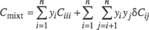
For a binary mixture,

(5-84)

As a result, C_mixt given by Eq. (5-84) is formally identical to the quadratic mole-fraction expression for the mixture’s second virial coefficient. Equation (5-84) requires only the same amount of data as that required for the calculation of second virial cross coefficients.

In Eq. (5-82), δC₁₂ is a binary parameter whose evaluation requires data for only one binary mixture. A single composition for a binary mixture is sufficient to calculate B₁₂ as well as C₁₁₂ and C₁₂₂, provided that we know C₁₁₁ and C₂₂₂.

Extension to multicomponent mixtures uses the assumption

(5-85)

Pairwise additivity is not assumed in Eq. (5-85). Rather, if is assumed that certain relations exist among the magnitudes of three-body interactions. Therefore, the simplifying assumptions expressed by Eqs. (5-82) and (5-85) reduce the number of interaction parameters required to obtain, e.g., compressibility factor z from Eq. (5-9). Thus, to evaluate z for a ternary mixture, Eqs. (5-21) and (5-23) require three cross terms for the second virial coefficients and seven for the third. However, the simplified model of McGregor, briefly described above, reduces to three the number of cross terms needed for the third virial coefficieat. In addition, McGregor’s method can be used to predict third virial cross coefficients when fitted to experimental data for a single binary mixture, thereby permitting the description of multicomponent mixtures using only data for binary mixtures.

Figure 5-26 Third virial coefficients [from Eq. (5-22)] for the mixture CH₄/CO₂ at 300 K. • Experiment; - · -· - Lennard-Jones; ---- Orbey and Vera; —— McGregor.

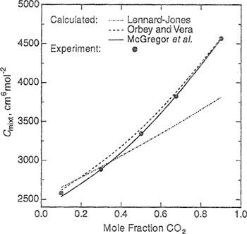
A comparison between experimental and calculated mixture third virial coefficients obtained from several methods has been presented by Brugge et al. (1989). They calculated C_mixt from Eq. (5-22) using the Lennard-Jones 6-12 intermolecular potential [C* = C*_add+ΔC*, where C* = C/(B*)²= C/(2/3πN_Aσ³);C^*_add is the pairwise contribution and ΔC* is the non-additivity correction], the empirical correlation of Orbey and Vera, and the model of McGregor. Figure 5-26 shows a comparison for the system methane/carbon dioxide at 300 K. Large deviations (particularly for high CO₂ concentrations) result from the calculations using the Lennard-Jones potential. In general, the other two methods are able to represent third virial coefficients of the mixtures within experimental uncertainty.

Quantum Gases. Corresponding-states correlations for virial coefficients may also be applied to quantum gases (helium, hydrogen, and neon) by using effective critical constants and ω = 0. Because the configurational properties of low-molecular weight molecules are described by quantum, rather than classical mechanics, effective critical constants depend on temperature. Following the method proposed by Gunn et al. (1966), these correlations for quantum gases use temperature dependent effective critical constants given by

(5-86)

(5-87)

(5-88)

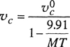
where M is the molar mass in grams per mole and T is in kelvin. Superscript ⁰ designates the “classical” critical constants that are the effective critical constants at high temperatures; as MT becomes large, T_c → T_c⁰, P_c → P_c⁰ and v_c → v_c⁰. Therefore, while Eqs. (5-86) to (5-88) are essentially empirical, they are consistent with the theoretical requirement that quantum corrections are important only for low-molecular weight compounds at low temperatures. Table 5-9 gives effective “classical” critical constants for neon and for isotopes of hydrogen and helium.

Table 5-9 “Classical” critical constants for quantum gases.

For mixtures containing one or more quantum gases, binary characteristic constants T_cij and P_cij are obtained from combining rules

(5-89)

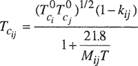
and

(5-90)

where

(5-91)

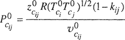
(5-92)

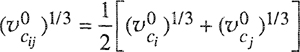
(5-93)

and

(5-94)

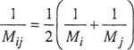
For a quantum gas, the effective ω = 0. For non-quantum gases, T_c⁰, P_c⁰ and v_c⁰ are the experimental critical temperature, pressure and volume. If no experimental value is available for the critical volume, it can be estimated by

The “classical” critical volumes listed in Table 5-9 satisfy this relation with ω = 0.

The combining rules listed above are useful for estimating cross-coefficient B_ij(i ≠ j) when either i or j (or both) is a quantum gas.

5.8 The “Chemical” Interpretation of Deviations from Gas-Phase Ideality

It was suggested many years ago that nonideal behavior of gases may be attributed to the formation of different chemical species. From the principle of Le Chatelier, one can readily show that, at low pressures, complex formation by association or solvation is negligible (resulting in ideal behavior); however, as pressure rises, significant chemical conversion may occur, sometimes leading to large deviations from ideal-gas behavior. For example, in pure gas A, various equilibria may be postulated:

2A A₂, 3A A₃, etc.

The equilibrium constant for dimerization reflects the interaction of two molecules at a time and therefore, a relation can be established between the dimerization equilibrium constant and the second virial coefficient (Mason and Spurting, 1969). Similarly, the trimerization equilibrium constant is related to the third virial coefficient, and so on. However, regardless of the degree of association, the “chemical” viewpoint considers the forces between molecules to be of chemical, rather than physical nature and it therefore attempts to explain nonideal behavior in terms of the formation of new chemical species. Polymerization reactions (dimerization, trimerization, etc.) result in negative deviations (z < 1) from ideal-gas behavior while dissociation reactions (primarily important at high temperatures) result in positive deviations (z >1).

5.9 Strong Dimerization: Carboxylic Acids

The “chemical” viewpoint is particularly justified for systems with strong forces of attraction between molecules; good examples are organic acids or alcohols and other molecules capable of hydrogen bonding. To illustrate, consider the dimerization of acetic acid:

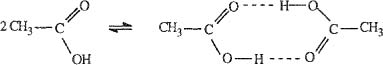
We define an equilibrium constant in terms of the partial pressures rather than fugacities because we assume that the mixture of true species (i.e., monomers and dimers) behaves as an ideal gas.

(5-95)

where P is the total pressure; y_A is the mole fraction of monomer; y_A2 is the mole fraction of dimer; and P⁰ is the standard-state pressure equal to 1 bar. The equilibrium constant can be calculated from P-V-T data as follows: We measure V, the volume for one mole of acetic acid at total pressure P and temperature T. (In this connection, one mole means the formula weight of monomeric acetic acid.) Let n_A be the number of moles of monomer and the number of moles of dimer; further, let α be the fraction of molecules that dimerize. Then n_T, the total number of “true” moles, is given by

(5-96)

with the restraint that n_A + 2n_A2 = 1, as required by material balance. Because, by assumption, PV = n_TRT, we can compute α by substitution and obtain

(5-97)

Because

(5-98)

and

(5-99)

the equilibrium constant K is related to a by

(5-100)

Equation (5-100) shows that, because K is a function only of temperature, a must go to zero as P approaches zero; in other words, dimerization decreases as the pressure falls. This pressure dependence of the degree of dimerization is a direct consequence of Le Chatelier’s principle.

Figure 5-27 gives dimerization constants for acetic acid and for propionic acid as a function of temperature based on experimental P-V-T measurements by McDougall (1936, 1941). In these gases, dimerization is very strong even at low pressures. For example, at 40°C and P = 0.016 bar, α for acetic acid is 0.8, and α for propionic acid is slightly larger, about 0.84. These gases show large deviations from ideal behavior at very low pressures, well below 1 bar.¹⁶. Tsonopoulos (1970) gives association constants for formic, acetic, propionic, butanoic, and trimethylacetic acids.

Figure 5-27 Dimerization equilibrium constants for acetic acid and propionic acid.

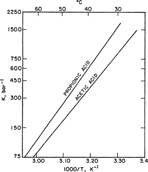
¹⁶ Because of strong dimerization in the vapor phase, the fugacity of a pure, saturated carboxylic acid is considerably lower than its saturation (vapor) pressure even when that pressure is small. Similarly, the fugacity coefficient of a carboxylic acid in a gaseous mixture is not close to unity even at low pressures. These deviations from ideal behavior are significant in vapor-liquid equilibria and failure to take them into account can lead to serious error. At low and moderate pressures, the fugacity of a strongly dimerized component, pure or in a mixture is set equal to the partial pressure of that component’s monomer; this partial pressure can be calculated from the dimerization equilibrium constant. Details of such calculations have been presented by various authors, notably by Sebastiani and Lacquanti (1967), Tsonopoulos (1970), and Marek (1954, 1955).

Because acetic and propionic acids are members of the same homologous series, it is reasonable to use the results shown in Fig. 5-27 to estimate the equilibrium constant for the solvation (or cross-dimerization) of these acids:

For this estimate, we assume that the enthalpy of the hydrogen bond is the same in the mixed dimer as that in either pure-component dimer. If A stands for acetic acid monomer and B stands for propionic acid monomer, we assume that there is zero enthalpy change for the reaction

However, the entropy change for this reaction is positive because distinguishability has been lost; whereas there are two different molecular species on the left side, there is only one molecular species on the right and therefore the reaction proceeds toward a more probable state. Details of the entropy calculation need not concern us here;¹⁷ the change in entropy is given by R1n2. The standard Gibbs energy of forming AB dimers from A and B monomers can now be calculated from the following scheme:

(5-101)

(5-102)

(5-103)

¹⁷ See R. Fowler and E. A. Guggenheim, 1952, Statistical Thermodynamics, p. 167, Cambridge: Cambridge University Press.

where is the molar Gibbs energy change in the standard state. Substitution gives .

From McDougall’s data at 20°C, , giving K_AB = 10.11×10^-3. Experimental measurements at 20°C by Christian (1957) indicate good agreement between the observed properties of acetic acid/propionic acid mixtures and those calculated from the three equilibrium constants. This favorable result is a fortunate consequence of the similar chemical nature of the mixture’s components; in other mixtures, where the solvating components are chemically dissimilar, it is usually not possible to predict accurately the properties of the mixture from data for the pure components.

Much attention has been given to the system acetic acid/water. For example, Tsonopoulos (1970) suggests that when the total pressure is near 1 bar, vapor-phase nonidealities can be described by the following chemical equilibria:

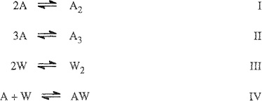
where A stands for acetic acid and W stands for water. Using P-V-T data, for acetic acid vapor, equilibrium constants are evaluated for I and II; using P-V-T (second virial coefficient) data for water vapor, an equilibrium constant is evaluated for III. For the cross-dimer, Tsonopoulos assumes that the equilibrium constant for IV is equal to that for III.

From material balances and from the four simultaneous chemical equilibria, Tsonopoulos calculates p_A, the partial pressure of acetic acid monomer and p_W, that of water monomer. The fugacity coefficients of (stoichiometric) water (1) and (stoichiometric) acetic acid (2) are then given by

(5-104)

(5-105)

Equations (5-104) and (5-105) follow from the general relation (see App. G) stating that, in an associated and/or solvated mixture, the chemical potential of a (stoichiometric) component is equal to that of the component’s monomer.

Figure 5-28 Vapor-phase fugacity coefficients for saturated mixtures of water (1)/acetic acid (2) at 1 bar.

Figure 5-28 shows calculated vapor-phase fugacity coefficients for the system water/acetic acid along the vapor-liquid saturation curve at 1 bar. The necessary dewpoint (T, y) data were taken from Sebastiani and Lacquanti (1967). Although the total pressure is low, deviations from ideal-gas behavior (φ₁ = φ₂ = 1) are large. In this calculation at 1 bar, chemical equilibrium I is by far the most important. If equilibria II, III, and IV had been neglected, the results shown in Fig. 5-28 would not be seriously affected.

5.10 Weak Dimerizations and Second Virial Coefficients

The “chemical” theory of virial coefficients was proposed many years ago; it has been extensively developed by Lambert (1953) and collaborators in connection with their studies of organic polar gases and polar-gas mixtures. Following Lambert, we consider a pure polar gas A and assume that the forces between A molecules can be divided into two classes: The first class is concerned with “normal” intermolecular forces (such as dispersion forces) that exist between nonpolar as well as polar molecules, and the second is concerned with chemical association forces leading to the formation of new chemical species. At moderate densities, the first class of forces is responsible for a “normal” or “physical” second virial coefficient, whereas the second class is responsible for a dimerization equilibrium constant. The equation of state is written

(5-106)

with

B = B_nonpolar + B_polar

Lambert has shown that B_polar is directly proportional to the dimerization equilibrium constant:

(5-107)

where P⁰ is the standard-state pressure (1 bar).

Techniques for calculating B_nonpolar are somewhat arbitrary bat, fortunately, this arbitrariness is not important for our purposes because, for any case where Lambert’s procedure is of interest, B_polar is always much larger in magnitude than B_nonpolar. A reasonable method for estimating B_nonpolar is to use the reduced second-virial-coefficient equation of Schreiber and Pitzer [Eq. (5-66)] with the true critical constants but with a fictitious acentric factor as determined by the polar molecule’s homomorph.¹⁸

¹⁸ The homomorph (homo = same, morph = form) of a polar molecule is a nonpolar molecule having essentially the same size and shape as those of the polar molecule. For example, the homomorph for acetonitrile coald be ethane.

However, dimerization can only account for negative second virial coefficients. While dissociation reactions can account for positive deviations from ideal-gas behavior, small positive deviations are commonly found for stable common gases (e.g. methane) at moderate pressures and at temperatures well above the critical; these deviations cannot realistically be ascribed to dissociation. For stable molecules at high reduced temperatures, positive second virial coefficients must be accounted for by the concept of excluded volume, i.e., the inaccessibility of some parts of space due to the finite size of the molecules.

In its simplest form, the excluded volume can be accounted for by an equation of state

(5-108)¹⁹

¹⁹ Equation (5-108) is equivalent to assuming that B_nonpolar = n_Tb_m

where V is the total volume, n_T is the true total number of moles, and n_Tb_m is the excluded volume due to the finite size of the molecules.

Let us suppose that, in the absence of any dimerization, there is one mole of A. As before, let α be the fraction of molecules that associate. Then, the equilibrium constant for association is given by Eq. (5-100); for small degrees of association (α << 1), Eq. (5-100) to a good approximation becomes

(5-109)

The gas is a mixture of monomer A and dimer A₂. Because we assume that α is much less than unity, is necessarily much smaller than n_A. Also, using Eqs. (5-96) and (5-109), the total number of moles present n_T is

(5-110)

Rewriting Eq. (5-108) gives

(5-111)

At modest densities, it is reasonable to assume that the excluded volume for the dimer is the same as that for the monomer. Therefore,

(5-112)

where b is the excluded volume for the monomer. Because the above derivation is based on one mole of A in the absence of any dimerization (i.e., n_A + 2n_A2 = 1), then n_Tb_m = b. This result and a comparison of Eq. (5-111) with Eq. (5-106) gives

(5-113)

Equation (5-113) was obtained for small degrees of dimerization (α << 1). Therefore, the chemical theory of gas imperfections leads to an equation of state of the virial form in the limit α → 0. Through Eq. (5-113) it is possible to obtain dimerization equilibrium constants from experimental second virial coefficients, provided that these coefficients were obtained at low densities where α is much less than unity. For highly polar fluids, and especially for strongly hydrogen-bonded fluids, the condition α << 1 is attained only at low pressures. To illustrate, consider acetic acid where α = 0.8 at 1600 Pa (or 0.016 bar) and 40°C; at the same temperature for α to be small, say equal to 0.01, it is necessary to reduce the pressure to 1.3 Pa. While carboxylic acids are unusually strong in their tendency to dimerize even at very low pressures, other common fluids (e.g., alcohols, aldehydes, esters, etc.) begin to dimerize to an appreciable extent only at normal pressures (close to 1 bar).

Lambert’s form of the virial equation of state is not useful for highly associating fluids because the valid pressure range for that equation is often extremely small. This limitation is not alleviated by introducing third (and higher) virial coefficients because these coefficients do not account for large α, but rather reflect the formation of trimers and higher aggregates.

In general, calculations based on the chemical theory of gas imperfections are not limited to small α; the theory holds for the entire range 0 ≤ α ≤ 1. In practice the chemical theory is limited to moderate pressures because, as pressure rises, trimer and higher aggregates are formed and few quantitative data are available on chemical equilibria beyond dimerization. For weakly interacting fluids (i.e. nonpolar or slightly polar components) there is little difference between results calculated from the chemical theory and those obtained from the “physical” virial equation. For some engineering applications, however, the chemical theory of gas imperfections presents an advantage over the virial equation because it is applicable to strongly polar and hydrogen-bonding fluids as well as to normal nonpolar fluids.

Experimental data for a large variety of polar gases have been reduced using the chemical theory described above, e.g. by Nothnagel et al. (1973) and by Olf et al. (1989a). When data are available over a range of temperature, a semilogarithrnic plot of K versus 1/T gives information on the enthalpy and entropy for dimer formation according to

(5-114)

The enthalpy Δh⁰ and entropy Δs⁰ of dimer formation in the standard state are obtained from experimental second virial coefficients using Eqs. (5-113) and (5-114). Excluded volume b in Eq. (5-113) is proportional to the volume of the molecules; for polyatomic molecules, b may be calculated from atomic radii and bond distances (Bondi, 1968). Some experimentally determined results are shown in Table 5-10 for several polar gases.

Table 5-10 Excluded volumes (obtained from the method of Bondi), standard enthalpies and entropies of dimerization (from second virial coefficients) for some polar gases.

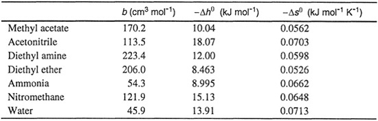
The “chemical” theory is readily extended to mixtures. A two-component mixture (say 1 and 2) contains five molecular species: A, A₂, B, B₂, and AB; their mole fractions are related by material balances and through three equilibrium constants, K_A2, K_B2, and K_AB; the first second of these can be determined from volumetric data for the pure components, as discussed above. However K_AB requires volumetric data for the mixture.

When dimerizations are weak, cross term B₁₂ of Eq. (5-20) is given by

(5-115)

In the above equation we assumed that [see Eq. (556)]. In the last term of Eq. (5-115), the factor 1/2 is a symmetry factor. When P-V-T data at low pressures are available for a binary mixture, it is then possible to find B₁₂ and hence K_AB. Figure 5-29 compares the temperature dependence of experimental second cross virial coefficients of methanol/methyl acetate and acetonitrile/methyl acetate with results calculated from chemical theory.

The equations presented above assume that chemical equilibria are limited to a stoichiometry of two (dimers). In principle, this assumption is not necessary but, with few exceptions, in practice the chemical theory is limited to moderate pressures where trimers (and higher aggregates) are neglected.²⁰

²⁰ A notable exception is hydrogen fluoride that forms hexamers. See, for example, M. Lencka and A. Anderko, 1993,AlChE J., 39: 533, and Sec. 12.10.

Figure 5-29 Second cross virial coefficients (Olf et al., 1989a) of methanol/methyl acetate and acetonitrile/methyl acetate. , m Experiment: –– Calculated from chemical theory.

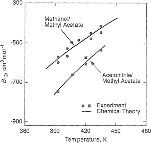
A few additional examples illustrate the “chemical” theory of gas nonideality for binary mixtures. First, we consider Carter’s data (1963) for the acetonitrile/acetaldehyde system. Carter found that the experimental second-virial cross coefficient for the mixture was much more negative than that of either pure component, as shown in Fig. 5-30; the magnitude of the cross-coefficient is unexpectedly large, much larger than that predicted by Stockmayer’s potential using pure-component parameters with common combining rules uncorrected for specific interactions. When Carter’s experimental data are used to calculate chemical equilibrium constants as described above, and when the temperature dependence of these constants is investigated using Eq. (5-114), the enthalpy of formation for the acetonitrile/acetaldehyde complex is considerably larger in magnitude than that for either pure-component dimer. The observed enthalpies are compared with theoretically calculated energies in Table 5-11.²¹

²¹ For our purposes here, no distinction need be made between energy and enthalpy.

The calculations are based on an electrostatic model with two structures, (a) and (b). In structure (a) the complex (or dimer) consists of two “touching” ideal spherical dipoles such that the dipoles are lined up in a direction perpendicular to the center-to-center separation, as shown at the bottom of Table 5-11. Structure (b) is similar, except that the dipoles are now lined up in a direction parallel to the center-to-center separation. From elementary electrostatic theory, the standard energy of formation of each of these structures is

(5-116)

(5-117)

Table 5-11 Standard energies of complex formation in the acetonitrile/acetaldehyde system (Carter, 1960).

Figure 5-30 Second virial coefficients for the acetonitrile/acetaldehyde system.

where μ is the dipole moment of the monomer, ε_o is the vacuum permittivity and r is the distance between the two centers of the two molecules that form the dimer. For acetonitrile and acetaldehyde the dipole moments are, respectively, 3.9 and 2.7 debye. Distances r were estimated from van der Waals radii reported by Pauling (1945).

The results in Table 5-11 suggest that the structure of the complex [structure (b), perhaps] is qualitatively different from that of the dimers that seem to have the properties of structure (a). In the absence of other experimental information, this interpretation of Carter’s data should not be taken too seriously but it does provide a possible explanation concerning why the cross-virial coefficient for this system is so different from the virial coefficients of the pure components.

For a second example consider the system ammonia/acetylene studied by Cheh et al. (1966). This system is qualitatively different from that studied by Carter because, while acetaldehyde and acetonitrile are both strongly polar, in the ammonia/acetylene system only ammonia has a dipole moment. Nevertheless, in the interaction between unlike molecules, there are strong complexing forces that are not present in the interactions between like molecules; Fig. 5-31 gives B₁₁, B₂₂, and B₁₂ and we see that B₁₂ is considerably more negative than either B₁₁ or B₂₂ Cheh et al., using appropriate potential functions, reduced the experimental second virial coefficients of the pure gases by taking into account all physical dispersion, induction, dipole, and quadrupole forces. Then, using conventional combining rules, they calculated the (physical) cross-coefficient B₁₂ and found that its magnitude was much too small, as shown in Fig. 5-32.

Figure 5-31 Experimental second viriai coefficients for acetylene (1) and for ammonia (2). B₁₂ is the observed cross coefficient for binary mixtures of (1) and (2).

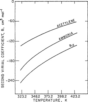
Figure 5-32 Second-virial cross coefficient for acetylene/ammonia mixtures. Calculated contributions from physical forces are insufficient to account for the observed large negative coefficient. B_12physical is the sum of contributions a, b, c and d.

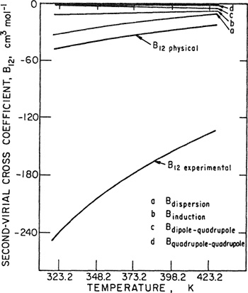
The high negative B₁₂ can be “explained” by the formation of a hydrogen bond between (acidic) acetylene and (basic) ammonia. This hydrogen-bond formation provides a reasonable explanation because there is much independent evidence for the basic properties of ammonia and there also is some independent evidence for the acidic properties of acetylene.²²

²² For example, acetylene is much more soluble in oxygen-containing solvents (such as acetone) than is ethane or ethylene.

Chemical equilibrium constant K for hydrogen-bond formation is found from

(5-118)

where P⁰ is the standard-state pressure (1 bar).

From the variation of K with temperature, the standard enthalpy and entropy of complex formation are

Δh⁰ = (-9250 ± 1250) J mol^-1

Δs⁰ = (-75.3 ± 3.8) J mol^-1 K^-1

These results are in good agreement with statistical-mechanical calculations for the formation of a loosely bonded complex of ammonia and acetylene.²³.

²³ The factor 1/2 in Eq. (5-118) was erroneously omitted in the work of Chen et al. (1966) and therefore the entropy reported there is in error by R In 2,

In some cases, specific chemical interaction between unlike molecules can lead to very large negative values for the second-virial cross coefficient B₁₂.

To illustrate, Fig. 5-33 shows some experimental results for the binary system trimethyl amine/methanol. The data of Millen and Mines (1974) indicate that there is strong interaction between the alcohol and the amine as suggested also by the shift in the (infrared) hydrogen-bond frequency of methanol (310 cm^-1 expressed in wave numbers). The enthalpy and entropy of complex formation are, respectively, -28.9 kJ mol^-1 and -98.3 J mol^-1 K^-1 at 25°C.

Figure 5-33 Second virial coefficients for the system trimethyl amine (1)/methanol (2).

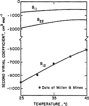
The large negative B₁₂ yields a remarkably low fugacity coefficient for methanol, infinitely dilute in trimethyl amine, as shown by Stein and Miller (1980). Figure 5-34 gives this fugacity coefficient at 45°C; even at low pressure, where gas-phase nonideality is usually negligible, the fugacity coefficient departs significantly from unity.

Figure 5-34 Fugacity coefficients for methanol at infinite dilution in trimethyl amine at 45°C (Stein and Miller, 1980).

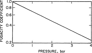
For calculating fugacity coefficients at moderate densities, it is desirable to have a correlation that includes both the “physical” contributions (second virial coefficients) and the “chemical” contributions (equilibrium constants) to vapor-phase nonideality. Hayden and O’Connell (1975), following earlier work by Nothnagel el al. (1973), presented a correlation of that form. Details of that correlation, including pertinent computer programs, are presented elsewhere.²⁴

²⁴ J. M. Prausnitz, T. F. Anderson, E. A. Grens, C. A. Eckert, R. Hsieh, and J. P. O’Connell, 1980, Computer Calculations for Multicomponent Vapor-Liquid and Liquid-Liquid Equilibria, Englewood Cliffs: Prentice Hall.

Figures 5-35 and 5-36 present fugacity coefficients for two binary systems, calculated with the Hayden-O’Connell correlation. In these calculations, application is directed at correlating isobaric vapor-liquid equilibria; the fugacity coefficients, therefore, are calculated at saturation, i.e., at dew-point conditions (Conti et al, 1960; Wisniak and Tamir, 1976). Although the total pressure is only 1 bar, deviations from ideal-gas behavior are considerable in both systems.

Figure 5-35 Fugacity coefficients for saturated mixtures of two carboxylic acids at 1 bar: formic acid (1)/acetic acid (2).

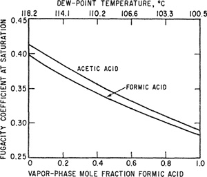
Figure 5-36 Fugacity coefficients for saturated mixtures of propionic acid (1)/methyl isobutyl ketone (2) at 1 bar.

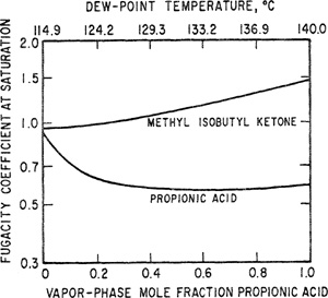
In the system formic acid/acetic acid, the fugacity coefficients are well below unity at all compositions because both components associate. In the system propionic acid/methyl isobutyl ketone, fugacity coefficients are close to unity only when the mole fraction of (associating) acid is small. As this mole fraction rises, deviations from ideal-gas behavior increase. The weak minimum in the fugacity coefficient for propionic acid is a consequence of two effects: As the concentration of acid rises, the tendency to associate increases but, because the temperature is also rising, the association constant decreases. At isobaric saturation, a change in composition is accompanied by a change in temperature. For propionic acid, an increase in mole fraction raises deviations from ideal-gas behavior but an increase in temperature lowers such deviations.

These examples illustrate that forces between molecules are often highly specific and in such cases it is unfortunately not possible to predict even approximately the properties of a mixture from those of the pure components. This is not surprising if we consider a far-fetched analogy: Let us suppose that a sociologist in Russia has carefully studied the behavior of Russians and after years of observation knows all about them. He then goes to China and makes a similar, thorough study of the Chinese. With this knowledge, can he then predict the behavior of a society where Russians and Chinese intermingle freely? Probably not. This analogy is highly extreme but serves to remind us that molecules are not inert particles floating blindly through space; instead, they are complicated “individuals” whose “personalities” are sensitive to their environment.

5.11 Fugacities at High Densities

Previous sections pointed out advantages of the virial equation of state but, as indicated earlier, this equation has an important disadvantage, i.e., its inapplicability to gases at high densities. The density range for practical application of the virial equation varies somewhat with the temperature, but frequently the virial equation is not useful at densities larger than about 50% of the critical (when third and higher virial coefficients are neglected) or 75% of the critical (when fourth and higher virial coefficients are neglected). This disadvantage follows primarily from our limited knowledge regarding third and higher virial coefficients.

At present, gas-phase fugacities at high densities can best be calculated by using semi-empirical methods.

For example, the theorem of corresponding states can be extended to mixtures utilizing what is often called the pseudocritical method introduced by Kay (1936). According to this method, the configurational properties of a mixture may be calculated from the generalized, reduced properties of pure fluids by expressing the characteristic reducing parameters as a function of mixture composition. This idea is easily illustrated by using the two-parameter corresponding-states theory that expresses compressibility factor z as a universal function of reduced temperature and reduced pressure,

(5-119)

The pseudocritical method assumes that the same universal function F_z applies to mixtures when T_c and P_c are taken, not as the (true) critical temperature and pressure of the mixture, but as pseudocritical constants, that is, characteristic parameters that depend on the composition of the mixture.

Kay assumed that T_c and P_c are linear functions of the mole fractions, although other functions relating T_c and P_c to composition are consistent with the pseudocritical idea (and numerous functions have been proposed by e.g. Reid and Leland, 1965; Leland and Chappelear, 1968). The pseudocritical and other empirical methods are reliable for many, but by no means all, cases. For example, for mixtures of small, nonpolar gases not near critical conditions, very good results can usually be obtained, while for mixtures containing polar components, reliability is frequently uncertain, and for all mixtures at or near critical conditions, regardless of molecular complexity, calculated fugacities are likely to be in error. These limitations follow directly from our incomplete knowledge of intermolecular forces between complex molecules and from our inability to describe in a simple way the behavior of fluids in the vicinity of the critical state.

The general and exact equations for the calculation of fugacities from volumetric properties have been derived and discussed in Chap. 3, and the two key relations are given again by Eqs. (5-1) and (5-2).

A more convenient method for calculating fugacities in gas mixtures is to use a phenomenological equation of state, i.e. an equation of state based on a molecular picture altough the details of the equation cannot be derived with theoretical rigor. Sometimes such equations are called semiempirical; most currently used phenomenological equations of state are based on a van der Waals-type picture of fluids.

While these equations of state are derived for pore fluids, they can be extended to mixtures upon making some simplifying assumptions. The key assumption is the one-fluid theory of mixtures. This theory assumes that the configurational properties of a mixture are the same as those of a hypothetical pure fluid whose characteristics (as expressed by constants in the equation of state) are some composition-dependent average of the characteristics of the pure components in the mixture.

The composition dependence of equation of state constants is given by mixing rules that are mostly empirical.

Given some phenomenological equation of state and using the one-fluid theory, we obtain a relation of the form

(5-120)

where υ is the molar volume of the mixture and a(y) and b(y) designate constants a and b as functions of mole fraction y. The number of such constants is arbitrary but, to keep experimental-data requirements low, typical useful equations of state contain no more than two or three substance-specific constants. These constants are often expressed in terms of critical temperature, critical pressure and acentric factor.

As shown in Chap. 3, Eq. (5-120) is sufficient to calculate fugacities of all components in a fluid mixture. Chapter 12 presents details concerning calculation of fugacities based on Eq. (5-120).

5.12 Solubilities of Solids and Liquids in Compressed Gases

Vapor-phase fugacity coefficients are required in any phase-equilibrium calculation wherein one of the phases is a gas under high pressure. If the gas is at low pressure, vapor-phase fugacity coefficients are usually close to unity, although there are some exceptions (e.g. acetic acid). However, vapor-phase fugacity coefficients are particularly important for calculating the solubility of a solid or a high-boiling liquid in a dense gas because in such cases failure to include corrections for gas-phase nonideality can lead to serious errors. To illustrate how corrections to gas-phase nonideality can significantly influence phase behavior, we now briefly present some examples concerning the solubility of a condensed component (a solid and a liquid) in a dense gas.

First, we consider equilibrium between a compressed gas and a solid. This is a particularly simple case because the solubility of the gas in the solid is almost always negligible. The condensed phase may therefore be considered pure and thus all nonideal behavior in the system can be attributed entirely to the vapor phase. Gas-liquid equilibria, considered later, is a little more complicated because the solubility of the gas in the liquid, while it may be small, is usually not negligible.

Let subscript 1 stand for the light (gaseous) component and let subscript 2 stand for the heavy (solid) component. We want to calculate the solubility of the solid component in the gas phase at temperature T and pressure P. We first write the general equation of equilibrium for component 2:

(5-121)

where superscript stands for the solid phase.

Because the solid phase is pure, the fugacity of component 2 is given by

(5-122)

as discussed in Sec. 3.3. In Eq. (5-122), is the saturation (vapor) pressure of the pure solid, the fugacity coefficient at saturation pressure and is the solid molar volume, all at temperature T.

For the vapor-phase fugacity, we introduce fugacity coefficient φ₂ by recalling its definition:

(5-123)

Substituting and solving for y₂, we obtain the desired solubility of the heavy component in the gas phase,

(5-124)

where

(5-125)

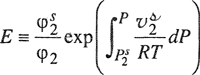
The quantity E, nearly always greater than unity, is called the enhancement factor; that is, E is the correction factor that must be applied to the simple (ideal-gas) expression valid only at low pressure. The enhancement factor provides a measure of the extent that pressure enhances the solubility of the solid in the gas; as P → , E → 1. It is a dimensionless measure of solvent power because it is the ratio of the observed solubility to the ideal-case solubility.

The enhancement factor contains three correction terms: takes into account nonideality of the pure saturated vapor; the Poynting correction gives the effect of pressure on the fugacity of the pure solid; and φ₂, the vapor-phase fugacity coefficient in the high-pressure gas mixture. Of these three correction terms, it is usually the last one that is by far the most important. In most practical cases, the saturation pressure of the solid is small and thus is nearly equal to unity. The Poynting correction is not negligible, but it rarely accounts for an enhancement factor of more than 2 or 3 and frequently much less. However, the fugacity coefficient φ₂ can be so far removed from unity as to produce very large enhancement factors that, in some cases, can exceed 10³ or more.

While enhancement factors in the range 10⁴-10⁶ are common, factors as high as 10¹² have been reported for the solubility of solid oxygen in dense gaseous hydrogen (McKinley et al., 1961).

Figure 5-37 shows the logarithm of the enhancement factor for solid carbon tetrachloride as a function of the density of supercritical carbon tetrafluoride at 249 K. The nearly linear function indicates that at high gaseous solvent densities (or pressures) very large deviations from nonideality are observed. The experimental data are fitted well using the Peng-Robinson equation of state (see Sec. 12.7).

Figure 5-37 Enhancement factors for solid CCl₄ in supercritical CF₄ at 249 K.

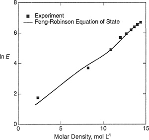
Another example of enhanced solubility of a solid in a dense gas is given in Fig. 5-38 that shows the solubility of solid carbon dioxide in compressed air at 143 K; the dashed line gives the calculated solubility with φ₂ = 1. In this calculation the solubility was calculated with the Poynting correction but with the assumption of gas-phase ideality. The two lines at the top of the diagram were calculated from Eq. (5-28) based on the virial equation; one calculation included only second virial coefficients, while the other included second and third virial coefficients. In these calculations air was considered to be a mixture of oxygen and nitrogen and therefore the results shown are those for a ternary system. The required virial coefficients were calculated from the Kihara potential using only pure-component parameters and customary combining rules. Calculated results are compared with experiment (Webster, 1952); when third virial coefficients are neglected, the calculations correctly predict the minimum in the curve of log y₂ versus P, but at pressures above that corresponding to the minimum mole fraction, third virial coefficients are required. In this particular system, agreement between calculated and experimental results at higher pressures is very good; unfortunately, such good agreement is not always obtained due to the difficulty of calculating third virial coefficients of mixtures. However, in the moderate-pressure region where third (and higher) virial coefficients can be neglected, it is almost always possible in nonpolar systems to make good estimates of the vapor-phase solubility of a solid (Ewald et al., 1953). Such estimates are frequently useful for engineering purposes; for example, in a freezing-out process it is desirable to minimize the mole fraction of a heavy impurity in a gas stream or, in a gas-cooling process, it is necessary to know the solubility of a heavy component to prevent plugging of the flow lines by precipitation of solid.

Figure 5-38 Solubility of solid carbon dioxide in air at 143 K.

At very high densities, the virial equation is not useful because almost no information is available on the fourth and higher virial coefficients; often, the second virial coefficient can be estimated well but the third virial coefficient can only be estimated approximately. Therefore, if the gas density is high (close to or exceeding the critical density), a mostly empirical equation of state must be used to relate the fugacity coefficient to the pressure, temperature, and gas-phase composition. To illustrate, Fig. 5-39 compares calculated (Kurnik and Reid, 1981) and experimental solubilities of naphthalene (melting point 80.2°C) in compressed ethylene as a function of temperature and pressure. The phase-equilibrium calculations shown in Fig. 5-39 were performed by Kurnik and Reid using the Peng-Robinson equation of state (see Sec. 12.3).

Figure 5-39 Solubility minima and maxima for naphthalene in compressed ethylene.

The results indicate S-shaped curves, each with a well-defined minimum at moderate pressure and a well-defined maximum at very high pressure. The maximum occurs at high densities when repulsive forces between ethylene and naphthalene become important; as the density (or pressure) rises further, naphthalene is “squeezed out” of the gaseous solution.

Kurnik and Reid have calculated maximum solubilities, shown by the dashed line in Fig. 5-40; the continuous lines indicate experimental data. The maximum solubility rises with increasing temperature because the vapor pressure of solid naphthalene rises with temperature. The pressure for maximum solubility falls with increasing temperature as we move away from the critical temperature of ethylene (282.4 K).

Figure 5-40 Solubility maxima for naphthalene in compressed ethylene.

Finally, consider the solubility of a liquid in a compressed gas. This situation is somewhat more difficult than that discussed above because a gas is soluble to an appreciable extent in a liquid, whereas the solubility of a gas in a solid is usually negligible. A general discussion of high-pressure vapor-liquid equilibria is given in Chap. 12; here we restrict ourselves to equilibrium between a high-boiling liquid and a sparingly soluble gas at conditions remote from critical. We are interested in the solubility of the heavy (liquid) component in the vapor phase that contains the light (gaseous) component in excess; as before, let 1 stand for the (light) gaseous solvent and 2 for the (heavy) solute in the gas phase. For the heavy component, the equation of equilibrium is where superscripts V and L stand, respectively, for vapor and liquid and where φ₂ is the vapor-phase fugacity coefficient of component 2 in the gaseous mixture.

(5-126)

Fugacity coefficient φ₂ must again be calculated from an equation of state, but before we turn to that calculation, we must say something about the fugacity of component 2 in the liquid phase. If the gas is only sparingly soluble, the liquid-phase fugacity of component 2 can be calculated by assuming that the solubility of component 1 in the liquid is described by a pressure-corrected form of Henry’s law (see Sec. 10.3): For component 1 we assume that, in the liquid phase, fugacity f₁^L is related to mole fraction x₁ by

(5-127)

where H_1,2 is Henry’s constant, is the partial molar volume of component 1 in the liquid phase at infinite dilution, and is the saturation pressure of pure liquid component 2, all at system temperature T. Then, from the Gibbs-Duhem equation, it can be shown that

(5-128)

where is the saturation pressure, is the fugacity coefficient at saturation, and is the molar volume, all of pure liquid 2, all at temperature T.

Substituting Eq. (5-128) into Eq. (5-126), and solving for the desired solubility y₂, we obtain

(5-129)

where x₁, the solubility of gas 1 in liquid 2, is calculated from

(5-130)

Solution of Eq. (5-129) necessarily requires a trial-and-error calculation because x₁ as well as φ₁ and φ₂ depend on the composition of the vapor. For the conditions under consideration, y₁ ≈ 1 and thus, as discussed in Sec. 5.1, the Lewis fugacity rule is a good approximation for the fugacity of component 1 (although it is a very bad approximation for the fugacity of component 2). For the first iteration, therefore, the calculations can be simplified by replacing φ₁ in Eq. (5-130) φ_{pure 1} (evaluated at the temperature and pressure of the system) and by setting y₂ = 0 in Eq. (5-28) for φ₂.

The fugacity of pure liquid 2 at temperature T and pressure P is readily calculated from the volumetric properties of pure component 2 as shown in Sec. 3.3. Henry’s constant H must be determined experimentally or else estimated from a suitable correlation (see Sec. 10.5); it need be known only approximately because, under the conditions considered, x₁ << 1, and thus even a somewhat inaccurate estimate of x₁ does not seriously affect the value of y₂. A rough estimate of is often sufficient here because the exponential correction to H may be small and often may be neglected.

In Eq. (5-129) it is the fugacity coefficient φ₂ that accounts for the nonideal behavior of liquid solubility in compressed gases. To illustrate, Fig. 5-41 shows the solubility of decane (normal b.p. 174°C) in compressed nitrogen at 50°C. Curve (a) gives calculated results assuming ideal-gas behavior and curve (c) shows results obtained when the Lewis fugacity rule is used for calculating the fugacity coefficient of decane (component 2). Curve (b) is based on the virial equation with B₁₂ = -141 cm³ mol^-1; it gives excellent agreement with experimental data (Prausnitz and Benson, 1959). Good agreement is perhaps not surprising because virial coefficient B₁₂ used in the calculation was back-calculated from the experimental solubility data. However, a reasonable estimate of B₁₂ could probably have been made without any data for this binary system by using one of the generalized equations discussed in Sec. 5.7.

Figure 5-41 Vapor-phase solubility of decane in nitrogen at 50°C.

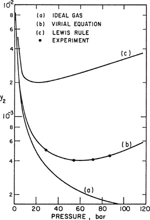
Nonideal behavior of the decane/nitrogen system at 50°C is not large because in this case the fugacity coefficient of decane is of the order of magnitude of unity (or, in other words, the absolute value of B₁₂ is not large). This result follows because nitrogen is a light gas with a potential energy much smaller than its kinetic energy at 50°C. Therefore, when a decane molecule escapes from the liquid into a space filled with gaseous nitrogen, it feels almost as if it were in a vacuum, or to put it more precisely, as if it were dissolved in an ideal gas. Thus the calculation based on the ideal-gas assumption is not seriously in error in this case; the solubility of decane in nitrogen is only a little larger than what it would be in an ideal-gas solvent because the attractive forces between solute and gaseous solvent are weak in this particular system at 50°C.

However, the ideal-gas assumption becomes increasingly bad for calculating the solubility of a liquid in a compressed gas when the potential energy of the gas is not small compared to its kinetic energy. To illustrate, Fig. 5-42 shows fugacity coefficients of decane at saturation in three gases. It is evident that the vapor-phase fugacity coefficient of decane (and hence its vapor-phase solubility) is strongly dependent on the nature of the gaseous component. Thus decane at 75°C and 100 bar is approximately 10 times more soluble in carbon dioxide than in nitrogen and approximately 40 times more soluble than in hydrogen. The relatively high solubility in carbon dioxide follows from the relatively large attractive forces between decane and carbon dioxide. A rough measure of the potential energy of a gaseous solvent is given by its critical temperature; therefore it is not surprising that carbon dioxide (T_c = 304.2 K) is a better solvent for decane than nitrogen (T_c = 126.2 K) that, in turn, is a better solvent than hydrogen (T_c = 33.3 K).

Figure 5-42 Fugacity coefficients of decane in hydrogen, nitrogen, and carbon dioxide at 75°C.

As a final example, Fig. 5-43 shows some second-virial cross coefficients for binary mixtures of methanol, obtained from vapor-phase solubility measurements (Lazalde-Crabtree et al., 1980). As the temperature falls, cross-coefficient B₁₂ becomes increasingly negative, corresponding to the rising importance of attractive forces between the dissimilar molecules. Attractive forces between methanol and nitrogen are weak compared to those between methanol and carbon dioxide.

Figure 5-43 Second-virial cross coefficients for binary mixtures containing methanol.

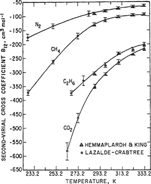
Methanol is an industrial solvent for sweetening natural gas by selective high-pressure absorption of the sour components carbon dioxide and hydrogen sulfide. Because of the solubility of methanol in the dense gas leaving the absorber, a high-pressure absorption process is necessarily accompanied by some solvent loss, that, at high flow rates, may represent an appreciable economic consideration. Figure 5-44 shows the calculated solubility of methanol in a typical effluent-gas mixture as a function of temperature and pressure. The calculations are based on equations of equilibrium similar to Eqs. (5-129) and (5-130) except that the necessary equations now are for a multicomponent, rather than a binary, mixture. For an industrial-scale natural-gas plant, the cost of solvent loss may be large, possibly a few million dollars per year.

Figure 5-44 Solvent loss in absorption. Solubility of methanol in a natural gas effluent.

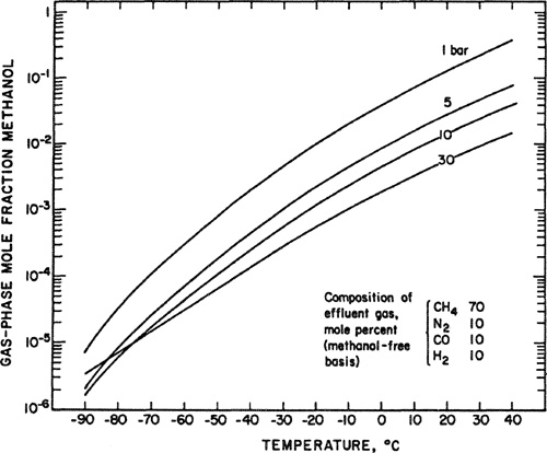
5.13 Summary

Efforts to describe quantitatively volumetric properties of real gases and gaseous mixtures extend over more than 200 years and the scientific literature abounds with articles on this subject. In this chapter we have given some of the main ideas with special reference to those contributions that appear to be most useful for technical applications. At the end of such a long chapter it is helpful to recapitulate and to state briefly the current status of efforts toward the calculation of gas-phase fugacities.

The fugacity of a component in a gas mixture at any temperature and density can be calculated exactly if volumetric data can be obtained for the mixture at the system temperature and over a density range from zero to the density of interest. However, because such data are rarely available, for practical purposes it is necessary to use approximations. A particularly simple approximation is provided by the Lewis fugacity rule; this rule is not generally reliable, although it gives good results for a component present in excess (Sec. 5.1).

There are many empirical equations of state and new ones continue to appear. These equations contain empirically determined constants and such constants have been reported for many common pure gases. To predict volumetric properties of a mixture, it is necessary to establish mixing rules that state how these constants depend on composition. For empirical equations of state, such mixing rules frequently cannot be established with confidence unless at least some data are available for the particular mixture of interest. Fugacity coefficients are usually sensitive to binary parameters in mixing rules.

A theoretically significant equation of state is the virial equation whose constants (virial coefficients) can be related to intermolecular potentials (Sees. 5.2, 5.3, and 5.4). The virial equation can readily be extended to mixtures; whereas for any pure component the virial coefficients depend only on temperature and on the intermolecular potential for that component, for a mixture they depend also on the potentials between molecules of those different components that comprise the mixture. The fundamental advantage of the virial equation is that it directly relates fugacities in mixtures to intermolecular forces. The practical disadvantage of the virial equation follows from insufficient understanding of intermolecular forces. As a result, we can at present apply the virial equation only to restricted cases: We can use it only for mixtures at moderate densities, and usually we can predict the required virial coefficients only for those mixtures whose components are nonpolar or weakly polar.

Many models for intermolecular potential functions have been proposed and from these, virial coefficients can be computed, provided that we can estimate the potential parameters (Sees. 5.5 and 5.6). For many practical purposes, however, it is simpler to calculate virial coefficients from correlations based on the theorem of corresponding states (Sec. 5.7).

For highly polar and hydrogen-bonded systems, virial coefficients can be interpreted “chemically” by relating them to the enthalpy and entropy of formation of chemically stable complexes (Sees, 5.8, 5.9, and 5.10). A “chemical” description of gas-phase nonideality is particularly useful for mixtures containing strongly hydrogen-bonded components like acetic acid.

Despite the limited practical use of the virial equation, we have devoted much attention to potential functions in this chapter because it is almost certain that in the future, fundamental advances in the description of volumetric properties will be based on research in statistical mechanics. Modern theories of fluids and molecular simulations require reliable potential functions.

At high densities, we must compute fugacity coefficients from mostly empirical equations of state or from generalized correlations such as those based on the theorem of corresponding states (Sec. 5.11). Research on the statistical mechanics of dense gases is progressing rapidly and we may expect practical results in the not-too-distant future; however, at present mostly empirical methods are more useful for most applications.

When applying an equation of state or a corresponding-states correlation to a gaseous mixture, flexibility in mixing rules is essential for good results. A mixing rule that is good for one system may not be good for another; mixing and combining rules should therefore contain one or two adjustable parameters determined, if possible, by a few data for the mixture under consideration. If no mixture data are available, they should be estimated by careful analysis of chemically similar systems where mixture data are at hand. Good estimates of fugacity coefficients can be made for constituents of dense gas mixtures that contain nonpolar (or slightly polar) components. However, for mixtures containing polar gases, or for any mixture near critical conditions, calculated fugacity coefficients are not likely to be highly accurate. Fugacity coefficients calculated from an equation of state are usually more sensitive to binary coefficients in mixing and combining rules than to any other detail in the equation of state, especially for those components that are dilute in the mixture.

In phase equilibria, the effect of gas-phase nonideality is particularly strong in those cases where a condensed component is sparingly soluble in a compressed gas. This solubility is strongly affected by the density and by the intermolecular forces between solute and gaseous solvent. In many cases, at high pressures, solubilities calculated with the assumption of ideal-gas behavior are in error by several orders of magnitude (Sec. 5.12).

We close this chapter by briefly repeating what we stressed at the beginning: Calculation of fugacities in gaseous mixtures is not a thermodynamic problem. The relations that express fugacity in terms of fundamental macroscopic properties are exact and well known; they easily lend themselves to numerical solution by computers. The difficulty we face lies in our inability to characterize and to predict with sufficient accuracy the configurational (essentially, volumetric) properties of pure fluids and even more, of mixed fluids; this inability, in turn, is a consequence of insufficient knowledge concerning intermolecular forces. To increase our knowledge, we require on the one hand new results from theoretical molecular physics and on the other, more accurate experimental data for equilibrium properties of dense mixtures, especially for those containing one or more polar components.

References

Axilrod, B. M. and E. Teller, 1943, J. Chem. Phys., II : 299.

Barker, J. A. and A. Pompe, 1968, Aust. J. Chem., 21: 1683.

Barker, J. A. and D. Henderson, 1976, Rev. Mod. Phys., 48: 587,

Besher, E. M. and J. Lielmezs, 1992, Thermochim. Acta, 200: 1.

Bondi, A., 1968, Physical Properties of Molecular Crystals, Liquids, and Glasses. New York: John Wiley & Sons.

Brugge, H. B., L. Yurttas, J. C. Holste, and K. R. Hall, 1989, Fluid Phase Equilibria, 51: 187.

Cheh, H. Y., J. P. O’Connell, and J. M. Prausnitz, 1966, Can. J. Chem., 44: 429.

Christian, S. D., 1957, J. Phys. Chem., 61: 1441.

Chueh, P. L. and J. M. Prausnitz, 1967, AIChE J., 13: 896.

Connolly, J. F. and G. A. Kandalic, 1960, Phys. Fluids, 3: 463.

Conti, J. J., D. F. Othmer, and R. Gilmont, 1960, J. Chem. Eng. Data, 5: 301.

Grain, R. W. and R. E. Sonntag, 1965, Adv. Cryog. Eng., 11: 379.

Cullen, E. J. and K. A. Kobe, 1955, AIChE J., 1:452.

De Santis, R. and B. Grande, 1979, AIChE J., 25: 937.

Douslin, D. R., 1962. In Progress in International Research on Thermodynamic and Transport Properties, (J. F. Masi and D. H. Tsai, Eds.). New York: ASME/Academic Press.

Dymond, J. H. and B. J. Alder, 1969, J. Chem. Phys., 51: 309.

Eubank, P. T. and K. R. Hall, 1990, AIChE J., 36: 1661.

Ewald, A. H., W. B. Jepson, and J. S. Rowlinson, 1953, Discuss. Faraday Soc., 15: 238.

Graben, H. W. and R. D. Present, 1962, Phys. Rev. Lett., 9: 247.

Guggenheim, E. A. and M. L. McGlashan, 1960, Proc. R. Soc. (Lond.), A255: 456.

Gunn, R. D., P. L. Chueh, and J. M. Prausnitz, 1966, AIChE J., 12: 937.

Hayden, J. G. and J. P. O’Connell, 1975, Ind. Eng. Chem. Process Des. Dev., 14: 204.

Hill, T. L., 1986, An Introduction to Statistical Thermodynamics. Reading: Addison-Wesley.

Hirschfelder, J. O., C. F. Curtiss, and R. B. Bird, 1954, Molecular Theory of Gases and Liquids. New York: John Wiley & Sons.

Joffrion, L. and P. T. Eubank, 1988, Fluid Phase Equilibria, 43: 263.

Kay, W. B., 1936, Ind. Eng. Chem., 28: 1014.

Kihara, T., 1953, Rev. Mod. Phys., 25: 831.

Kihara, T., 1958, Adv. Chem. Phys., 1: 276.

Kihara, T., 1963, Adv. Chem. Phys., 5: 147.

Kurnik, R. T. and R. C. Reid, 1981, AIChE J., 27: 861.

Lambert, J. D., 1953, Discuss. Faraday Soc., 15: 226.

Lazalde-Crahtree, H., G. J. F. Breedveld, and J. M. Prausnitz, 1980, AIChE J., 26: 462.

Leland, T. W. and P. S. Chappelear, 1968, Ind. Eng. Chem., 60: 15.

Mak, P. C. N. and J. Lielmezs, 1989, Ind. Eng. Chem. Res. 28: 127.

Marek, J., 1954, Collect. Czech. Chem. Comm., 19: 1074.

Marek, J., 1955, Collect. Czech. Chem. Comm., 20: 1490.

Mason, E. A. and T. H. Spurling, 1969, The Virial Equation of State. In The International Encyclopedia of Physical Chemistry and Chemical Physics. Elmsford: Pergamon Press.

Mayer, J. E. and M. G. Mayer, 1977, Statistical Mechanics, 2^nd Ed. New York: Wiley Interscience.

McDougall, F. H., 1936,. J. Am. Chem. Soc., 58: 2585.

McDougall, F. H., 1941, J. Am. Chem. Soc., 63: 3420.

McGlashan, M. L. and D. J. B. Potter, 1962, Proc. R. Soc. (Lond.), A267: 478.

McGlashan, M. L. and C. J. Wormald, 1964, Trans. Faraday Soc., 60: 646.

McGregor, D. R., J. C. Holste, P. T. Eubank, and K. R. Hall, 1987, Fluid Phase Equilibria, 35: 153.

McKinley, C., J. Brewer, and E. S. J. Wang, 1961, Adv. Cryog. Eng., 7: 114.

Meissner, H. P., and R. Seferian, 1951, Chem. Eng. Prog., 47: 579.

Michels, A., J. M. Levelt, and W. DeGraff, 1958, Physica, 24: 659.

Michels, A., W. DeGraaff, and C. A. Ten Seldam, 1960, Physica, 26: 393.

Millen, D. J. and G. M. Mines, 1974, J. Chem. Soc. Faraday Trans. II, 70: 693.

Munn, R. J., 1964, J. Chem. Phys., 40: 1439.

Munn, R. J. and F. J. Smith, 1965, J. Chem. Phys., 43: 3998.

Munn, R. J. and F. J. Smith, 1965a, Discuss. Faraday Soc., 40.

Myers, A. L. and J. M. Prausnitz, 1962, Physica, 28: 303.

Nothnagel, K. H., D. S. Abrams, and J. M. Prausnitz, 1972, Ind. Eng. Chem. Process Des. Dev., 12:25.

O’Connell, J. P. and J. M. Prausnitz, 1968, J Phys. Chem., 72: 632.

Olf, G., A. Schnitzler, and J. Gaube, 1989, Fluid Phase Equilibria, 49: 49.

Olf, G., J. Spiske, and J. Gaube, 1989a, Fluid Phase Equilibria, 51: 209.

Orbey, H. and J. H. Vera, 1983, AIChE J., 29: 107.

Orentlicher, M. and J. M. Prausnitz, 1967, Can. J. Chem., 45: 373.

Patel, M. R., J. C. Holste, K. R. Hall, and P. T. Eubank, 1987, Fluid Phase Equilibria, 36: 279.

Pauling, L., 1945, The Nature of the Chemical Bond. Ithaca: Cornell University Press.

Pope, G. A., P. S. Chappelear, and R. Kobayashi, 1973, J. Chem. Phys., 59: 423.

Prausnitz, J. M. and P. R. Benson, 1959, AIChE J., 5: 161.

Prausnitz, J. M. and W. B. Carter, 1960, AIChE J., 6: 611.²⁵ See also Renner, T. A. and M. Blander, 1977, J. Phys. Chem., 81: 857.

²⁵ The equilibrium constants reported here are too large by a factor of 1.317. However, the enthalpies of complex-formation are not affected.

Prausnitz, J. M. and R. N. Keeler, 1961, AIChE J., 7: 399.

Prausnitz, J. M. and A. L. Myers, 1963, AIChE J., 9: 5.

Reid, R. C. and T. W. Leland, 1965, AIChE J., 11: 229.

Riedel, L., 1956, Chem.-Ing.-Tech., 28: 557 (and earlier papers).

Rossi, J. C. and F. Danon, 1966, J. Phys. Chem., 70: 942.

Rowlinson, J. S., 1949, Trans. Faraday Soc., 45: 974.

Rowlinson, J. S., 1951, J. Chem. Phys., 19: 827.

Rowlinson, J. S., 1955, Trans. Faraday Soc., 51: 1317.

Rowlinson, J. S., 1965, Discuss. Faraday Soc., 40: 19.

Schreiber, D. R. and K. S. Pitzer, 1989, Fluid Phase Equilibria, 46:113.

Sebastiani, E. and L. Lacquanti, 1967, Chem. Eng. Sci., 22: 1155.

Sherwood, A. E. and J. M. Prausnitz, 1964. J. Chem. Phys., 41: 429.

Sherwood, A. E. and J. M. Prausoifz, 1964a. J. Chem. Phys., 41: 413.

Sherwood, A. E., A. G. DeRocco, and E. A. Mason, 1966, J. Chem. Phys., 44: 2984.

Stein, F. P. and E. J. Miller, 1980, Ind. Eng. Chem. Process Des. Dev., 19: 123.

Stogryn, D. E., 1968, J. Chem. Phys., 48: 4474.

Stogryn, D. E., 1969, J. Chem. Phys., 50: 4667.

Stogryn, D. E., 1970, J. Chem. Phys., 52: 3671.

Tarakad, R. R. and R. P. Danner, 1977, AlChE J., 23: 685.

Tsekhanskaya, Y. V., M. B. Iomtev, and E. V. Mushkina, 1964, Zh. Fiz. Chim., 38: 2166.

Tsonopoulos, C. and J. M. Prausnitz, 1970, Chem. Eng. J., 1: 273.

Tsonopoulos, C., 1974, AIChE J., 20: 263.

Tsonopoulos, C., 1975, AIChE J., 21: 827.

Tsonopoulos, C., 1978, AIChE J., 24: 1112.

Tsonopoulos, C. and J. L. Heidman, 1990, Fluid Phase Equilibria, 57: 261.

Van Welie, G. S. A. and G. A. M. Diepen, 1961, J. Rec. Trav. Chim., 80: 673.

Webster, T. J, 1952, Proc. R. Soc. (Lond.), A214: 61.

Wisniak, J. and A. Tamir, 1976, J. Chem. Eng. Data, 21: 88.

Problems

1. Consider the following simple experiment: We have a container of fixed volume V; this container, kept at temperature T, has in it n₁ moles of gas 1. We now add isothermally to this container n₂ moles of gas 2 and we observe that the pressure rise is ΔP. Assume that the conditions are such that the volumetric properties of the gases and their mixture are adequately described by the virial equation neglecting the third and higher coefficients. The second virial coefficients of the pure gases are known. Find an expression that will permit calculation of B₁₂.

2. At -100°C, a gaseous mixture of one mole contains 1 mol % CO₂ and 99 mol % H₂. The mixture is compressed isothermally to 60 bar. Does any CO₂ precipitate? If so. approximately how much? [At -100°C, the saturation (vapor) pressure of pure solid CO₂ is 0.1392 bar and the molar volume of solid CO₂ is 27.6 cm³ mol^-1.]

3. A gaseous mixture containing 30 mol % CO₂ and 70 mol % CH₄ is passed through a Joule-Thomson expansion valve. The gas mixture enters the valve at 70 bar and 40°C and leaves at 1 bar. Does any CO₂ condense? Assume that the heat capacities are independent of temperature. The data are as follows (1 = CH₄; 2 = CO₂):

B₁₁ = 42.5 – 16.75×l0³T^-1 – 25.05 × 10⁵T^-2

B₂₂ = 40.4 – 25.39×10³T^-1 – 68.7×10⁵T^-2

B₁₂ = 41.4 – 19.50×10³T^-1 – 37.3×10⁵T^-2

where B is in cm³ mol^-1 and T is in K. The c_p⁰ for an ideal gas are: c_p⁰_.1 = 35.8 J mol^-1 K^-1 and c_p⁰_.2 = 37.2 J mol^-1 K^-1. The vapor pressure equation for pure CO₂ is

4. On the basis of the Stockmayer potential, devise a corresponding-states theorem for polar substances. How many reducing parameters are there, and what are they?

5. Using the generalized correlations of Pitzer (or Lee and Kesler), calculate:

(a) The energy of vaporization of acetylene at 0°C.

(b) The second virial coefficient of a mixture containing 80 mol % butane and 20 mol % nitrogen at 461 K. (The experimental value is -172 cm³ mol^-1).

(c) The enthalpy of mixing (at 200 K and 100 bar) of one mole of methane, one mole of nitrogen, and one mole of hydrogen.

6. A gas stream at 25°C consists of 40 mol % nitrogen, 50 mol % hydrogen, and 10 mol % propane. The propane is to be removed from this stream by high-pressure absorption using a mineral oil of very low volatility. At the bottom of the column (where the gas enters), what is the driving force for the rate of absorption? The total pressure is 40 bar. The driving force for a component i is given by

Driving force = p_i – p_i*

where p_i is the partial pressure of i in the gas bulk phase and p_i* is the partial pressure of i in the gas phase in equilibrium with the liquid phase. In this column the liquid-to-gas flow ratio (L/G) is five moles of liquid per mole of gas. The column is to absorb 95% of the propane. Solubility of inert gases in the mineral oil is negligible. The data are as follows: The compressibility factor of the entering gas mixture is 0.95. The solubility of propane in the mineral oil is given by f_c3 = Hx_c3 with H = 53.3 bar at 25°C.

7. A gas mixture contains 2 mol % ethane (1) and 98 mol % nitrogen (2). The ethane is to be recovered by absorption into heavy oil at 40°C and 50 bar. When this gas mixture is in equilibrium with the oil, what is the relative volatility α_2,1 of nitrogen to ethane?

Data, all at 40°C, are as follows:

Henry’s constant for nitrogen in the oil: 1000 bar

Henry’s constant for ethane in the oil: 100 bar

Second viriai coefficients (cm³ mol^-1): B₁₁ = -172; B₂₂ = -1.5; B₁₂ = -44.

Partial molar volumes in the oil (cm³ mol^-1); nitrogen, 25; ethane, 60.

8. At 0°C and pressures to 20 bar, the solubility of methane (1) in methanol (2) follows Henry’s law; Henry’s constant is 1022 bar. The vapor pressure of methanol at 0°C is 0.0401 bar. Second viriai coefficients (cm³ mol^-1) at 0°C are B₁₁ = -53.9, B₁₂ = -166, and B₂₂ = -4068. At 0°C and 20 bar, what is the solubility (mole fraction) of methanol in methane? Why is this solubility of interest in chemical engineering?

9. Acetic acid vapor has a tendency to dimerize. Show that in an equilibrium mixture of monomer and dimer the fugacity of the dimer is proportional to the square of the fugacity of the monomer.

10. Compare the systems:

hydrogen chloride/diisopropyl ether

hydrogen chloride/ethyl butyl ether

Second-virial cross coefficients B₁₂ are available for both systems at 70°C. Compare the two coefficients. Are they likely to be positive or negative? Which one is more positive? Why?

11. At 143.5°C, the saturation (vapor) pressure of acetic acid is 2.026 bar. The dimerization constant for acetic acid at this temperature is 1.028 bar^-1. The molar liquid volume of acetic acid at 143.5°C is 57.2cm³ mol^-1. Calculate the fugacity of acetic acid at 143.5°C and 50 bar (see App. B).

12. The viriai equation gives the compressibility factor as an expansion in the density

(1)

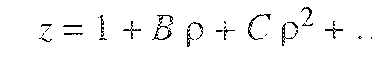
Because it is more convenient to use pressure as an independent variable, another form of the viriai equation is given by

(2)

(a) Relate the viriai coefficients B’ and C to the constants a and b that appear in the Redlich-Kwong equation.

(b) Consider a binary gas mixture of ethylene and nitrogen having mole fraction y_C2H4 = 0.2. Starting with Eq. (2), calculate the fugacity of ethylene at 50°C and 50 bar. Neglect viriai coefficients beyond the second. For the second viriai coefficient, use the relation found in (a) for the Redlich-Kwong equation with the customary mixing rules. (From experimental volumetric data, the fugacity of ethylene, under the conditions specified, is 8.87 bar.)

13. One mole of a binary gas mixture containing ethylene and argon at 40°C is confined to a constant-volume container. Compute the composition of this mixture that gives the maximum pressure. Assume that virial coefficients beyond the second may be neglected.

14. 100 moles of H₂ initially at 302.6 K and 20.7 bar is mixed adiabatically and isobarically with 2000 moles of ethylene initially at 259.5 K and 20.7 bar. What is the temperature of the final mixture?

15. A metallic sheet is to be coated with a thin layer of an organic solid A. To do so, it is proposed to vaporize the solid and to allow the vapor to condense on the sheet in an isolated chamber, as indicated below:

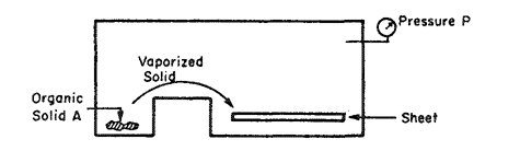
The condensation rate depends on the partial pressure of A. Since A is thermally unstable, it can be heated to no more than 350 K, where its vapor pressure is 1 torr. To increase the rate of condensation, it is proposed to fill the chamber with carbon dioxide gas at high pressure. What total pressure should the chamber have so that the partial pressure of A is 10 torr? Assume that the entire chamber is isothermal at 350 K and that the volumetric properties of CO₂-A mixtures are given by

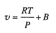
where B is the second virial coefficient and v is the volume per mole of mixture. At 350 K, for pure A, B = -500; for pure CO₂, B = -85 and the cross-coefficient B_A-CO2 = -430, all in units of cm³ mol^-1. The molar volume of solid A at 350 K is 200 cm³ mol^-1.

16. At 35°C the vapor pressure of solid naphthalene is 2.80×10^-4 bar and its density is 1.145 g cm^-3. Calculate the solubility of naphthalene in compressed ethylene at 35°C and at total pressure of 30 bar:

(a) Using the ideal-gas law.

(b) Using the virial equation of state truncated after the second term For the second virial coefficient B use the van der Waals result,

Van der Waals constants a and b are related to the critical constants. For the gas mixture assume that a and b are a quadratic and a linear function of the mole fraction, respectively.

17. Moist air at 30 bar is cooled isobarically to -10°C. What is the maximum permissible moisture content (mole fraction gaseous water) that the air may have to be sure that no moisture condenses? Assume that the volumetric properties of moist air at 30 bar are given by the virial equation of state truncated after the second term. For this calculation, assume that dry air is 80 mol % nitrogen and 20 mol % oxygen.

Second virial coefficients at -10°C are (cm³ mol^-1): B₁₁ = -25; B₂₂ = -12; B₃₃ = -1500; B₁₂ = -15; B₁₃ = -63; B₂₃ = -53, where 1 stands for nitrogen, 2 for oxygen, and 3 for water. At -10°C, the vapor pressure of ice is 1.95 torr and the density of ice is 0.92 g cm^-3.

18. At 300 K and modest pressures, the joule-Thomson coefficient of hydrogen is negative (i.e., upon isenthalpic expansion, hydrogen becomes warmer). How much ethane must be added (per mole of hydrogen) to produce a Joule-Thomson coefficient of zero at 300 K and modest pressure? Use the truncated-virial equation with the correlation of McGlashan and Potter. Use the following reducing parameters (where 1 stands for hydrogen and 2 for ethane):

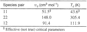
19. A subterranean natural-gas reservoir is at 60°C and 20 bar. The gas (primarily methane) is in contact with liquid water. The gas is pumped from the well to a pipeline operating at 40 bar and 25°C. Assuming that there is no entrainment of liquid water in the gas stream from the well, estimate the amount of liquid water [in moles of liquid water (2) removed per mole of methane (1) produced] that must be removed from the methane stream in the pipeline. Data:

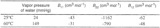
20. An equimolar mixture of CO₂ and CH₄ at 50 bar and 298 K is to be separated into pure CO₂ at 50 bar and 298 K and pure CH₄ at 50 bar and. 298 K by a continuous Slow process involving heat interactions with the environment at 298 K. Calculate the minimum possible amount of work per mole of mixture that would be required for this separation. Assume that the gases follow the volume-explicit form of the virial equation of state, truncated after the second virial term, both in the pure state and in the mixtures. Second-virial coefficient data are (1 = CH₄; 2 = CO₂; B in cm³ mol^-1 and T in kelvin):

B₁₁ = 42.5 – 16.75×l0³T^-1 – 25.05 × 10⁵T^-2

B₁₂ = 40.4 – 25.39×10³T^-1 – 68.7×10⁵T^-2

B₂₂ = 41.4 – 19.50×10³T^-1 – 37.3×10⁵T^-2

21. Using the square-well potential, find the fugacity of methyl chloride at 150°C and 30 atm. Potential parameters are: ε/k = 469 K; σ = 0.429 nm; R (well width) = 0.337σ.

Also calculate the enthalpy and entropy of dimerization of methyl chloride in the dilute-gas phase. For the entropy of dimerization, use an ideal-gas standard state of 1 mol L^-1.

22. Consider a gas for which the intermolecular potential Γ(r) is given by

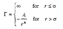
where A and n are constants.

(a) Obtain an expression for the second virial coefficient of this gas at high temperature.

(b) Determine allowable values of n in this expression and the relationship of dB/dT with the attractive part of the potential.

23. Assume that argon at 273.15 K is represented by the square-well potential with ε/k = 141.06 K, σ = 0.2989 nm, and R = 1.55. Estimate the second virial coefficient for argon at 273.15 K and compare with the experimental value B = -22.08 cm³ mol^-1.

24. The Sutherland potential describes the interaction introduced by van der Waals in his equation. Using the data below, obtain B(T) for methane and n-pentane given by the Sutherland potential. Compare with experimental second-virial-coefficient data at 373 K.

For methane: ε/k = 434.8 K; σ = 0.3294 nm; 3(373 K) = -20 cm³ mol^-1.

For n-pentane: ε/k = 1096.8 K; σ = 0.4755 nm; B(373 K) = -621 cm³ mol^-1.

25. A closed chamber, maintained at 40°C, consists of two equal parts, separated from each other by a membrane permeable only to helium. Each part has a volume of 300 cm³. The pressure in the left part is 37.5 bar and the pressure in the right part is 84.5 bar. The left part is filled with 0.99 moles ethane and 0.01 moles helium; the right part is filled with 0.99 moles nitrogen and 0.01 moles helium. After equilibrium is attained, what are the mole fractions of helium in each part of the chamber?

Assume that the virial equation truncated after the second term is applicable. The following second virial coefficients (cm³ mol¹) are available (where 1 stands for helium, 2 for ethane, and 3 for nitrogen):

B₁₁ = 17.17; B₁₂ = 24.51

B₂₂ = -169.23; B₁₃ = 21.97

B₃₃ = -1.55; B₂₃ =-44.39

26. Hydrogen fluoride associates in the gas phase; two possibilities are under consideration:

(a)

(b)

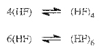
To test these possibilities, the vapor-phase densities of HF were measured at two pressures at 50°C. They are

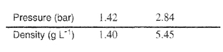
In view of these measurements, which possibility, (a) or (b), is more likely? The molar mass of HF is 20 g mol^-1.