Chapter 12
High-Pressure Phase Equilibria

Numerous chemical processes operate at high pressures and, primarily for economic reasons, many separation operations (distillation, absorption) are conducted at high pressures; further, phase equilibria at high pressures are of interest in geological exploration, such as in drilling for petroleum and natural gas. While the technical importance of high-pressure phase behavior has been recognized for a long time, quantitative application of thermodynamics toward understanding such behavior was not common until about 1940. In the early days of phase-equilibrium thermodynamics, such an attempt could not be made because of computational complexity; realistic thermodynamic calculations for high-pressure equilibria are difficult without computers.

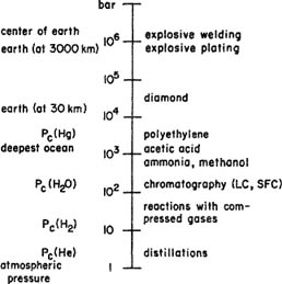
The adjective high-pressure is relative; in some areas of technology (e.g., outer-space research) 1 mm of mercury is a high pressure whereas in others (e.g., solid-state research) a pressure of a few hundred bars is considered almost a vacuum. Figure 12-1 (Schneider, 1976) shows a rough comparison between pressures observed in nature and pressures of some common industrial processes. For pure fluids, critical pressures can vary from 2.3 bar (for helium) to 1500 bar (for mercury); the pressure at the bottom of the deepest ocean (about 10 km deep) is about 1150 bar, while at the center of the earth the pressure is estimated to be larger than 4×10⁶ bar. On the other hand, for man-made processes, high-pressure techniques can require pressures like 5×10⁴ bar (synthesis of diamonds), or even 10⁶ bar, as in explosive welding and plating, sophisticated techniques used in the production of tubing for chemical reactors. Pressures between 100 and 1000 bar are used in high-pressure liquid chromatography and in supercritical fluid chromatography, for hydrogenation processes, and for synthesis of products like ammonia, methanol, and acetic acid. Classical production of low-density polyethylene occurs at pressures between 1500 and 3000 bar.

Figure 12-1 Pressure scale for natural (left) and chemical (right) processes (Schneider, 1976).

For the description of these and similar processes, it is necessary to understand the thermodynamic properties of fluids at high pressures, as discussed in this chapter. We designate here as “high-pressure” any pressure sufficiently large to have an appreciable effect on the thermodynamic properties of all the phases under consideration. In vapor-liquid equilibria, a high pressure may be anywhere between (about) 20 to 1000 bar, depending on the system and on the temperature; only in rare cases does the pressure exceed 1000 bar, because in most cases of common interest the vapor-liquid critical condensation pressure of the system is below 1000 bar. In liquid-liquid equilibria or in gas-gas equilibria the pressure may be considerably larger, although experimental studies are rare for fluid mixtures at pressures beyond 1000 bar.

12.1 Fluid Mixtures at High Pressures

Before discussing the thermodynamic relations that govern the behavior of mixtures at high pressures, let us take a brief look at some typical results to obtain a qualitative picture of how mixed fluids behave at pressures well above atmospheric.

For vapor-liquid behavior of a typical simple system, consider mixtures of ethane and n-heptane; the critical temperature of ethane is 32.3°C and that of n-heptane is 267.0°C. Figure 12-2 shows the relation between pressure and composition at 149°C. The left-hand line gives the saturation pressure (bubble pressure) as a function of liquid composition and the right-hand line gives the saturation pressure (dew pressure) as a function of vapor composition. The two lines meet at the critical point where the two phases become identical. At 149°C the critical composition is 76 mol % ethane and the critical pressure is 88 bar. At this temperature and composition, therefore, only one phase can exist at pressures higher than 88 bar; further, regardless of pressure, it is not possible to have at 149°C a coexisting liquid phase containing more than 76 mol % ethane.

Figure 12-2 Pressure-composition diagram for the system ethane/n-heptane at 149°C. The critical point of the mixture is at C (Mehta and Thodos, 1965).

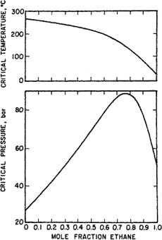
To characterize vapor-liquid equilibria for a binary system, measurements like those shown in Fig. 12-2 must be repeated for other temperatures; for each temperature, there is a critical composition and critical pressure. Figure 12-3 gives experimentally observed critical temperatures and pressures as a function of mole fraction for the ethane/n-heptane system. While the critical temperature of this system is a monotonic function of composition, the critical pressure goes through a maximum; many, but by no means all, binary systems behave this way.

Figure 12-3 Critical temperatures and pressures for the system ethane/n-heptane (Mehta and Thodos, 1965).

For typical technical calculations it is convenient to express phase-equilibrium relations in terms of K factors; by definition K ≡ y/x, the ratio of the mole fraction in the vapor phase y, to that in the liquid phase x. The definition of K has no thermodynamic significance but K is commonly used in chemical engineering calculations where it is convenient for writing material balances.

Figure 12-4 shows experimental K factors for the two components of the methane/propane system (Sage and Lacey, 1938). The lines for propane start at the saturation pressure for pure propane (where K = 1), decrease with rising pressure and, after going through minima, rise to K = 1 at the critical point. For methane, K factors decrease in the entire pressure range to K = 1 at the critical point.

Figure 12-4 K factors for the methane/propane system (Sage and Lacey, 1938).

Because Figs. 12-2 to 12-4 are for simple systems, they do not indicate the variety of phase behavior that is possible in binary systems. That variety increases substantially when we consider also partial immiscibility of liquids and possible occurrence of solid phases, as discussed in the next sections.

12.2 Phase Behavior at High Pressure

To understand phase behavior at high pressure, we need to know how to calculate and interpret phase diagrams.

Calculation of phase diagrams is based on solving the equation of phase equilibrium; for vapor-liquid equilibrium,

f_i^V = f_i^L

for every component i in the mixture.

To interpret phase diagrams we need Gibbs’ phase rule. We cannot here give a complete discussion; we provide only an introduction. For a review of phase equilibrium diagrams for binary mixtures at high pressures, including a description of experimental and theoretical methods, see, for example, Hicks and Young (1974); Rowlinson and Swinton (1982); Sadus (1992); and Schouten (1992).

Interpretation of Phase Diagrams

To interpret phase diagrams we apply the Gibbs phase rule (see Sec. 2.5). For nonreacting systems, that rule is expressed by the simple relation,

(12-1)

where the number of independent variables (or degrees of freedom) F is related to the number of components m and number of phases π. However, at a critical point, the physical properties of the coexisting phases become identical, Criticality therefore imposes an additional π — 1 constraints that reduce the number of degrees of freedom given by Eq. (12-1). The number of degrees of freedom of a gas-liquid critical point is zero for a one-component system; for a two-component system, the number of degrees of freedom is one (a line), and for a three-component system it is two (a surface).

Pressure and temperature are the most convenient independent variables for the measurement and study of phase equilibria in fluid systems. In fluid systems, changes in pressure and temperature produce large changes in the phase behavior and a three-dimensional diagram in pressure, temperature and a third variable is required for a complete description of a two-component system (see Table 12-1). For qualitative descriptions and comparisons of phase diagrams, the most convenient choice for this third variable is the composition z, where z designates the composition of a phase of any kind (solid, liquid, or gas). Pressure-temperature-composition (P-T-z) diagrams provide a basis for the design of separation processes such as distillation and extraction. Therefore, three-dimensional drawings are commonly used, together with two-dimensional diagrams cut by planes of constant T or P, or formed by projections of lines and points on the P-T coordinate plane.

Table 12-1 Geometric constraints imposed by the phase rule on phase equilibria.

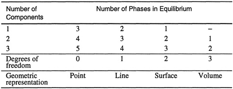
The phase rule is a useful guide for construction and interpretation of phase diagrams; it imposes definite constraints on the geometry of the features that describe the existence and coexistence of a fixed number of phases.¹ For example, Eq. (12-1) tells us that for a two-component system with 3 phases in equilibrium, phase equilibria are represented by lines; phase equilibria for a 1-component system is fully described in a 2-dimensional diagram that contains points, lines, and surfaces, corresponding to the equilibria of, respectively, 3 phases, 2 phases, and 1 phase. Table 12-1 summarizes the results of the phase rule for different types of systems.

¹ A useful concept for the analysis of phase-equilibrium diagrams is the distinction between two types of variables: field variables and density variables. Field variables are those that take identical values for each phase when two (or more) phases are in equilibrium, such as pressure, temperature, and chemical potential. Density variables are those that have different values for each phase, such as density, enthalpy, and composition.

Table 12-1 shows that a system of n phases in equilibrium is described by n geometrical features of the appropriate type: a one-component system of three phases is described by three points, a two-component system of three phases is described by three lines, etc. The interpretation of (high pressure) phase diagrams is an important aspect for the proper design and operation of many chemical engineering processes.

Classification of Phase Diagrams for Binary Mixtures

As Table 12-1 shows, complete description of a two-component system requires three-dimensional P-T-z diagrams (a combination of two field variables, P and T, and one density² variable, composition z). In two-component systems, regions of two-, three-and four-phase equilibria are described in P-T-z space by pairs of surfaces, triplets of lines, and quadruplets of points, respectively. However, the geometrical constraints imposed by two field variables require (Rowlinson and Swinton, 1982) that these features have common P-T projections, i.e., two surfaces representing two coexisting phases project as a single surface, three lines representing three coexisting phases project as a single line, etc.

² See Footnote 1.

Van Konynenburg and Scott (1980) showed that almost all known types of binary fluid-phase equilibria (vapor-liquid, liquid-liquid, and gas-gas equilibria) can be qualitatively predicted using the van der Waals equation of state³ and quadratic mixing rules. Their calculations suggested the classification of binary fluid-phase behavior into six types, based on the shape of the mixture critical line and on the absence or presence of three-phase lines. However, due to limitations of the equation of state used, they were able to generate only five of these six types with the van der Waals equation of state. A brief description of each of these types of phase behavior is presented below. More complete descriptions can be found elsewhere (Rowlinson and Swinton, 1982; Schneider, 1978; McHugh and Krukonis, 1994; Sadus, 1994).

³ Phase diagrams of binary fluid mixtures have been calculated also from other equations of state, namely from those of Redlich-Kwong (Deiters and Pegg, 1989), Camahan-Starling-Redlich-Kwong (Kraska and Deiters. 1992), and those based on the simplified-pertutbed-hard-chain equation (van Pelt et al, 1991).

Type I-Phase Behavior

To illustrate the variety of phase behavior in binary mixtures, Fig. 12-6 shows a few schematic pressure-temperature diagrams for binary systems. These diagrams are P-T projections of the P-T-z surface, shown schematically in Fig. 12-5 for a typical type I-mixture.

Figure 12-5 P-T-z surface and corresponding P-T projection showing vapor-liquid equilibria for a simple binary mixture (type I).

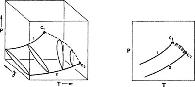
Figure 12-6 Six types of phase behavior in binary fluid systems. C = critical point; L = liquid; V = vapor; UCEP = upper critical end point; LCEP = lower critical end point. Dashed curves are critical lines and hatching marks heterogeneous regions.

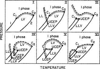
In the simple case shown in Fig. 12-5, the line ending at C₁ is the vapor-liquid coexistence curve for pure 1 while the line ending at C₂ is the vapor-liquid coexistence curve for pure 2; C₁ and C₂ are the critical points. The dashed line joining these points is the critical locus; each point on that line is the critical point for a mixture of fixed composition. The continuous vapor-liquid critical line and the absence of liquid-liquid immiscibility is often observed for mixtures where the two components are chemically similar and/or their critical properties are comparable. Typical examples are methane/ethane, carbon dioxide/n-butane, and benzene/toluene. The critical locus may (but need not) show either a minimum or a maximum. The latter is an indication of large positive deviations from Raoult’s law and hence of relatively weak, unlike intermolecular interactions; such behavior is found for binary mixtures of, e.g., a polar with a non-polar fluid, such as methanol/n-hexane.

Type II-Phase Behavior

Type II is similar to type I except that, at low temperatures, liquid mixtures of components 1 and 2 are not miscible in all proportions. There is thus one additional critical line. The line labeled LLV gives the locus of a three-phase line where one vapor phase is in equilibrium with two liquid phases. This locus ends at the upper critical end point⁴ (UCEP) where the two liquid phases merge into one liquid phase; the pressure of the UCEP depends on temperature as shown in Fig. 12-6 by the dashed line curving upward, in this case, with a negative slope. This negative slope indicates that the upper critical solution temperature (see Sec. 6.13) decreases with rising pressure. The phase diagrams of type II-mixtures may be complicated by the presence of an azeotropic line. However, the essential feature of this type (and also of type VI-mixtures) is the continuous vapor-liquid critical line that is distinct from the liquid-liquid critical line. Examples of type II are carbon dioxide/n-octane and ammonia/toluene. As shown, the critical line starting at C₂ has an initial negative slope but that is not always so; the slope may initially be positive and become negative at higher pressures. Further, the 3-phase line LLV may in some cases reside above the vapor pressure-curve of component 1, as observed for mixtures of hydrocarbons with the corresponding fully- or near fully-fluorinated fluorocarbons, e.g. methane/trifluoromethane.

⁴ Critical end points are limiting end points where two of three coexisting phases become identical.

Type III-Phase Behavior

For mixtures with large immiscibility such as water/n-alkane mixtures, the locus of the liquid-liquid critical lines moves to higher temperatures and may then interfere with the vapor-liquid critical curve. This means that the vapor-liquid critical locus is not necessarily a continuous line connecting C₁ and C₂, as illustrated in type III. In this type, the critical locus has two branches. One branch goes from the vapor-liquid critical point of the more volatile component, C₁, to UCEP, where the gaseous phase and the liquid phase (richer in the more volatile component) have the same composition. The other branch starts at C₂ and then rises with pressure, perhaps with a positive slope (e.g., helium/water) or with a negative slope (e.g., methane/toluene) or with a slope that changes sign (e.g., nitrogen/ammonia and ethane/methanol). The critical line starting from C₂ with a positive slope indicates the existence of what is called gas-gas equilibria: two phases at equilibrium at a temperature larger than the critical temperature of either pure component. Gas-gas immiscibility is conveniently classified as either first kind (almost exclusively confined to mixtures containing helium as one component, e.g. water/helium and helium/xenon) where the critical curve extends directly from the critical point of the less volatile component with a positive slope; or second kind, where the critical line passes first through a temperature minimum and then goes steeply to increasing temperatures and pressures (e.g., methane/ammonia and water/propane).

Experimentally, an unambiguous distinction between, e.g., a type-II and a type-III P-T projection is accomplished by direct visual observation to determine the two of the three equilibrium phases that merge at the three-phase LLV critical point. As shown in Fig. 12-6, if the two liquid phases merge in the presence of the equilibrium vapor phase, then the P-T projection is of type II; if the vapor phase and one liquid phase merge in the presence of the second equilibrium liquid phase, then the P-T projection is of type III. Therefore, the type of P-T projection is given by observation of the disappearance of one of the two menisci separating the three equilibrium phases, as well as critical opalescence, at the three-phase critical endpoints. Experimentally, this visualization is usually carried out in a high-pressure view cell equipped with windows (typically sapphire) that allow the visual observation of phase separation, the number of coexisting phases, and critical opalescence.⁵

⁵ See, e.g., S. P. Christensen and M. E. Paulaitis, 1992, Fluid Phase Equilibria, 7: 63; E. Gomes de Azevedo, H. A. Mates, and M. Nunes da Ponte, 1993, Fluid Phase Equilibria, 83: 193.

Type IV-Phase Behavior

Type IV is similar to type V. In both, the vapor-liquid critical line starting at C₂ ends at a LCEP, a terminal point of the LLV three-phase line. However, in type IV the LLV locus has two parts; this means that there is limited liquid-phase miscibility at low temperatures, ending at UCEP. As the temperature and pressure rise, there is a second region of limited miscibility from LCEP to UCEP. Such phase behavior is shown by ethane/1-propanol and carbon dioxide/nitrobenzene.

Type V-Phase Behavior

In type V, the first branch of the critical line goes from C₁ to UCEP as in type III, but the second branch goes from C₂ to the lower critical end point (LCEP). Contrarily to type IV, in type V mixtures, the liquids are completely miscible below LCEP. Figure 12-7 gives a schematic representation of what is visually observed at the LCEP and at the UCEP. Two liquid phases exist only for temperatures between those of the critical endpoints. At the temperature of the LCEP, the meniscus between the two liquids disappears, whereas at that of the UCEP, it is the gas-liquid interface that disappears leaving in both cases one liquid phase in equilibrium with a gas phase.

Figure 12-7 Three-phase behavior and schematic representation of critical end points for the binary ethane/n-octadecane (Specovius et al., 1985). The dashed line represents a disappearing meniscus, i.e., a critical point: gas-liquid at the UCEP (39.30°C) and liquid-liquid at the LCEP (39.14°C).

Mixtures of n-alkanes with large size differences show type-V phase behavior. While the binary methane/n-pentane shows type-I phase behavior, type-V behavior occurs in the system methane/n-hexane. With ethane as the lighter component, n-octadecane is the first long n-alkane to exhibit partial miscibility in the liquid state, only 7°C above the critical temperature of ethane (t_c = 32.2°C), as illustrated in Fig. 12-7. The immiscible region for ethane/n-octadecane extends over a very narrow temperature range (0.157°C) and all phases are rich in ethane. This temperature range increases to 2.927°C for the binary ethane/n-eicosane, (C₂₀H₄₂) while complete miscibility is observed for ethane/n-heptadecane.

Type V phase behavior is also found in binaries containing alcohols. An example is provided by ethylene/methanol whose phase behavior is shown in Fig. 12-8.

Figure 12-8 Phase-behavior of ethylene (1)/methanol (2): (a) Experimentally obtained P-T projection (note the scale change in the temperature axis at about 300 K, required by the large difference between the volatilities of the two components). —— Vapor-pressure curves of the pure components; - - - - critical lines; — - — - LLV three-phase line; (b) to (e) P-X isotherms at the temperatures indicated.

From the P-T projection represented in Fig. 12-8(a), several P-x diagrams were derived at four characteristic temperatures. At temperature T_i, there is a normal gas-liquid equilibrium [Fig. 12-8(b)]. When the temperature of the LCEP is exceeded, a L₁L₂ region begins to grow out of the bubble curve [Fig. 12-8(c)]. The liquid phase L₁ is rich in methanol and liquid phase L₂ is rich in ethylene. At the critical temperature of pure ethylene, the two-phase L₂-V region separates from the axis corresponding to , and forms an additional critical point [Fig. 12-8(d)]. As the temperature increases further, the L₂-V region becomes smaller until it disappears at the temperature of the UCEP (see Fig. 12-7); regions L₁-V, L₁-L₂, and L₂-V fuse with each other and a normal V-L equilibrium with a supercritical component is now present [Fig. 12-8(e)].

By observing the phase changes at the successive boundaries encountered in the P-T projection of a binary mixture (illustrated here for the type-V binary ethylene/methanol), we are able to construct the corresponding isothermal P-x diagrams (Sadus, 1992). For comparison, Fig. 12-9 shows experimental phase-equilibrium measurements for the same binary at 260, 273, 284.15, and 298.15 K. The 284.15 K isotherm, 2.7 K below the temperature of the UCEP, shows the three two-phase regions L₁-V, L₁-L₂, and L₂-V. Because at this temperature the L₂-V region is very small (extends only over a pressure interval of 0.9 bar and over an ethylene mole fraction interval of 0.04), it is difficult to detect experimentally. The 298.15 K isotherm is 11.3 K above the temperature of the UCEP; it shows only a typical V-L equilibrium with ethylene in the supercritical state. The flat boiling curve observed in the 260 K isotherm suggests two-liquid splitting starting at 263.55 K.

Figure 12-9 Pressure-composition phase-equilibrium data for ethylene/methanol at 260 K and 273 K (Zeck and Knapp, 1986) and at 284 K and 298 K (Brunner, 1985).

Type VI-Phase Behavior

Finally, binary mixtures showing type-VI phase behavior have two critical curves: One connects C₁ and C₂ while another connects UCEP and LCEP. It is the presence of the LCEP that distinguishes type-VI from type-II systems. The closed dome of immiscibility formed between LCEP and UCEP is a consequence of the opposite signs of the slopes (dT_LCEP/dP)_x and (dT_UCEP/dP)_x. The two critical curves meet at an upper critical pressure; at higher pressures two liquids are miscible. Examples of this complex behavior are found in mixtures where one (or both) component is self-associated through hydrogen bonding. An example of type VI is water/2-butanol.

Critical Phenomena in Binary Fluid Mixtures

It is a challenge to devise quantitative models that can reproduce fluid-phase behavior as shown in Fig. 12-6 that introduces only some (by no means all) observed phase diagrams. In principle, it should be possible to calculate such diagrams from an equation of state. Van Konynenburg and Scott (1980) have shown that the original van der Waals equation (with conventional mixing rules) can be used to calculate qualitatively nearly all of the observed phase diagrams for binary nonelectrolytes. However, if attention is restricted to conventional equations of state, calculation of such diagrams in quantitative agreement with experiment is at present possible only for type I and type II phase behavior. As better equations of state become available and as computing techniques improve, it is likely that accurate phase diagrams will be calculated not only for all types of binary mixtures but also for multicomponent systems (Sadus, 1992).

While Fig. 12-6 shows only binary fluid phases, some experimental data are also available for binary high-pressure systems where solid phases exist in addition to fluid phases, but we shall not pursue that topic here.

Figure 12-6 gives different types of pressure-temperature diagrams for binary systems with variable composition. When a pressure-temperature diagram is constructed for a simple binary mixture at fixed composition, we have a bubble-point (boiling) curve on the left and a dew-point (condensation) curve on the right, as shown in Fig. 12-10. These two curves come together at the critical point. The dashed lines in Fig. 12-10 are lines of constant quality.⁶ At the bubble-point line, the entire mixture is liquid and at the dew-point line, the entire mixture is vapor.

⁶ In a two-phase (vapor-liquid) mixture, quality is defined as the fraction that is in the vapor phase.

Figure 12-10 Pressure-temperature diagrams for a pure fluid (a) and for fluid mixtures at constant composition (b, c, d). BPL= bubble-point line; DPL = dew-point line; C = critical point. Dashed lines show constant quality.

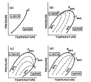
For a pure fluid, the bubble-point and dew-point curves collapse into one single line; in that event, the critical point is a maximum in the sense that it is at the highest temperature and pressure where liquid and vapor can coexist at equilibrium. However, in a mixture, the critical point is not necessarily a maximum with respect to either temperature or pressure. In a mixture, liquid and vapor may coexist at equilibrium at temperatures and pressures higher than those corresponding to the critical point. The relative positions of C, T_max, and P_max (see Fig. 12-10) give rise to a curious but well-known phenomenon: retrograde condensation.

Normally, when we compress a vapor mixture at constant temperature, liquid starts to form at the dew point; as compression proceeds, more liquid is formed until (at the bubble point) all vapor has been condensed. However, in the vicinity of the mixture’s critical point, isothermal compression may proceed such that an isotherm cuts the dew-point line not once, but twice and does not cut the bubble-point line at all. Such an isotherm is shown in Fig. 12-11.

Figure 12-11 Retrograde condensation. The vertical line cuts the dew-point line twice. BPL = bubble-point line; DPL = dew-point line; C = critical point. When gaseous mixture e is compressed isothermally, liquid begins to form at d; maximum condensation occurs at c, and at b, all condensate is vaporized. Dashed lines show constant quality.

Suppose a vapor mixture is at e. It is isothermally compressed. The first liquid is formed at d. More liquid is formed until c; thereafter, liquid evaporates until, at b, all liquid is evaporated. Conversely, if we start with a vapor-phase mixture at a and expand isothermally, the first liquid is obtained at b; more liquid is formed until c and thereafter, liquid evaporates until all of the mixture is again vapor at d.

Similar unexpected effects can be obtained by isobarically cooling or heating a mixture in the critical region. Retrograde phenomena are common in natural-gas reservoirs where proper understanding of retrograde behavior is important for efficient gas production.

Phase behavior of liquid mixtures containing only subcritical components is also affected by pressure, but in this case much higher pressures are usually required to produce significant changes. For example, at ordinary pressures, the system methyl ethyl ketone/water has an upper critical solution temperature and a lower critical solution temperature; in between these temperatures, the two liquids are only partially miscible. As observed by Timmermans (1923), increasing pressure lowers the upper critical solution temperature and raises the lower critical solution temperature as indicated in Fig. 12-12(a).

Figure 12-12 Liquid-liquid phase behavior for different binary mixtures (Timmermans, 1923; Schneider, 1966). Lower and upper consolute temperatures as functions of pressure for: (a) methyl ethyl ketone/water; (b) triphenylmethane/sulfur; (c) 2-methylpyridine/deuterium oxide; (d) 4-methylpiperidine/water.

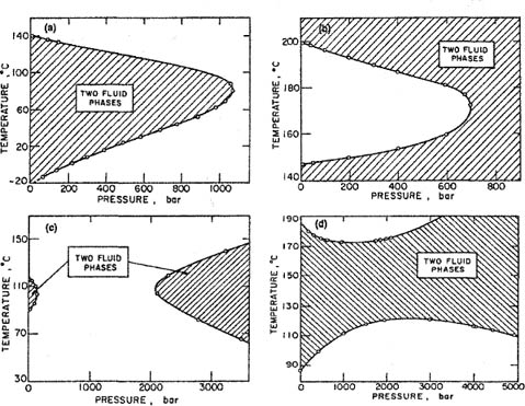
As pressure rises, the region of partial miscibility decreases and at pressures beyond 1100 bar, this region has disappeared. By contrast, the system triphenylmethane/sulfur exhibits the opposite behavior; in this case, increasing pressure reduces the region of complete miscibility as indicated by Fig. 12-12(b). Finally, Figs. 12-12(c) and 12-12(d) illustrate two additional types of phase behavior. Figure 12-12(c) shows that for the system 2-methylpyridine/deuterium oxide, increasing pressure first induces miscibility and then, at still higher pressures, produces again a region of incomplete miscibility. On the other hand, Fig. 12-12(d) shows that for the system 4-methylpiperidine/water, increasing pressure does not eliminate the region of partial miscibility; very high pressures, after first causing this region to shrink, bring about an increase in the two-phase region. Connolly (1966) has observed behavior similar to that shown in Fig. 12-12(c) for some water/hydrocarbon systems.

Figures 12-2 to 12-12 illustrate only some of the types of phase behavior at high pressures; many other phase phenomena have been observed for binary systems and, when ternary systems are considered, additional phase phenomena become possible, as discussed elsewhere (Rowlinson and Swinton, 1982; Sadus, 1992; Schneider, 1993; de Swaan Arons and de Loos, 1994).

12.3 Liquid-Liquid and Gas-Gas Equilibria

Before examining high-pressure equilibria in systems containing one liquid phase and one vapor phase, we briefly consider the effect of pressure on equilibria between two liquid phases and later, between two gaseous phases.

Liquid-Liquid Equilibria

To illustrate the effect of pressure on liquid-liquid equilibria, Fig. 12-13 shows experimental results for the system carbon tetrafluoride/propane. In this case, rising pressure increases the size of the two-phase region; in other words, rising pressure is unfavorable for miscibility. Thermodynamics can help us to interpret results such as those shown in Fig. 12-13. In particular, we want to examine how pressure may be used to induce miscibility or immiscibility in a binary system.

Figure 12-13 Pressure (a) and temperature (b) dependence of liquid-liquid equilibria in the system carbon tetrafluoride/propane (Jeschke and Schneider, 1982).

Two liquids are miscible in all proportions if Δ_mixg, the molar Gibbs energy of mixing at constant temperature and pressure, satisfies the relations

(12-2)

and

(12-3)

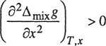
for all x. Because Δ_mixg is a function of pressure, it follows that under certain conditions, a change in pressure may produce immiscibility in a completely miscible system or, conversely, such a change may produce complete miscibility in a partially immiscible system. The effect of pressure on miscibility in binary liquid mixtures is closely connected with the volume change on mixing, as indicated by the exact relation

(12-4)

where Δ_mixυ is the volume change on mixing at constant temperature and pressure.

To fix ideas, consider a binary liquid mixture that at normal pressure is completely miscible and whose isothermal Gibbs energy of mixing is given by curve a in Fig. 12-14. Suppose that for this system Δ_mixυ is positive; an increase in pressure raises Δ_mixg, and at some higher pressure the variation of Δ_mixg with x₁ may be given by curve b. As indicated in Fig. 12-14, Δ_mixg at the high pressure no longer satisfies Eq. (12-3) and the liquid mixture now has a miscibility gap in the composition interval x^'₁ < x₁ < x^"₁.

Figure 12-14 Effect of pressure on miscibility: a - low pressure, no immiscibility; b - high pressure, immiscible for x^'₁ < x₁ < x^"₁.

For contrast, consider also a binary liquid mixture that at normal pressures is incompletely miscible as shown by curve a in Fig. 12-15. If Δ_mixυ for this system is negative, then an increase in pressure lowers Δ_mixg and at some high pressure the variation of Δ_mixg with x₁ may be given by curve b, indicating complete miscibility. It follows from these simple considerations that the qualitative effect of pressure on phase stability of binary liquid mixtures depends on the magnitude and sign of the volume change of mixing. To carry out quantitative calculations at some fixed temperature, it is necessary to have information on the variation of Δ_mixυ with x and P in addition to information on the variation of Δ_mixg with x at a single pressure.

Figure 12-15 Effect of pressure on miscibility: a - low pressure, immiscible for x^'₁ < x₁ < x^"₁; b - high pressure, no immiscibility.

To illustrate, we consider a simple, symmetric binary mixture at some fixed temperature and 1 bar pressure. For this liquid mixture, we assume that

(12-5)

(12-6)

where A and B are experimentally determined constants. Further, we assume that the liquid mixture is incompressible for all values of x; i.e., we assume that B is independent of pressure. At any pressure P, we have for Δ_mixg,

(12-7)

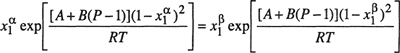
where P is in bar. Substituting Eq. (12-7) into Eq. (12-3), we find that the mixture is partially immiscible when

(12-8)

Equation (12-8) tells us that if A/RT < 2 (complete miscibility at 1 bar) and if B > 0, then there is a certain pressure P (larger than 1 bar) where immiscibility is induced. On the other hand, if A/RT > 2 (incomplete miscibility at 1 bar) and if B < 0, then there is a certain pressure P (larger than 1 bar) where complete miscibility is attained.

When two liquid phases exist, the compositions of the two phases α and β are governed by equality of fugacities for each component:

(12-9)

(12-10)

If the same standard-state fugacities are used in both phases, Eqs. (12-9) and (12-10) can be rewritten using activity coefficient γ:

(12-11)

(12-12)

For the simple mixture described by Eqs. (12-5) and (12-6), we can calculate activity coefficients as discussed in Chapter 6; we substitute into Eqs. (12-11) and (12-12) and we then obtain

(12-13)

(12-14)

Simultaneous solution of these equilibrium relations (coupled with the conservation equations and ) gives the coexistence curve for the two-phase system as a function of pressure.⁷

⁷ Because of symmetry, Eq. (12-13) and Eq. (12-14) are always satisfied by the trivial solution A useful method for solving Eqs. (12-13) and (12-14) is given by Van Ness and Abbott, 1982, Classical Thermodynamics of Nonelectrolyte Solutions, New York: McGraw-Hill.

Experimental studies of liquid-liquid equilibria at high pressures were reported many years ago by Roozeboom (1918), Timmermans (1923) and Poppe (1935). Schneider and coworkers (Dahlmann, 1989; Becker, 1993; Ochel et al, 1993; Wallbruch, 1995; Grzanna, 1996), and the thermodynamic group at Delft (Bijl et al., 1983; Gregorowicz et al., 1993; de Loos et al., 1996) have reported similar experimental work.

Winnick and Powers (1963, 1966) made a detailed study of the acetone/carbon disulfide system at 0°C; at normal pressure, this system is completely miscible. For an equimolar mixture the volume increase upon mixing is of the order of 1 cm³ mol^-1, a fractional change of about 1.5%. Winnick and Powers measured the volume change on mixing as a function of both pressure and composition; these measurements, coupled with experimentally determined activity coefficients at low pressure, were then used to calculate the phase diagram at high pressures, using a thermodynamic procedure similar to the one outlined above. The calculations show that incomplete miscibility should be observed at pressures larger than about 3800 bar. Winnick and Powers also made experimental measurements of the phase behavior of this system at high pressures; they found, as shown in the lower part of Fig. 12-16, that their observed results are only in approximate agreement with those calculated from volumetric data. Good quantitative agreement is difficult to achieve because the calculations are extremely sensitive to small changes in Δ_mixg, the Gibbs energy of mixing, as shown in the upper part of Fig. 12-16. As indicated by Eqs. (12-3) and (12-4), a small change in the volume change on mixing has a large effect on the second derivative of Δ_mixg with mole fraction.

While gas-gas equilibria are rare, liquid-liquid equilibria are common; as briefly discussed in Sec. 6.13, critical phenomena can exist in liquid-liquid system as well as in liquid-vapor systems. In a binary system, the gas-liquid critical temperature depends on pressure, as illustrated in Fig. 12-3. Similarly, in a binary system with limited liquid-phase miscibility, the liquid-liquid critical temperature also depends on pressure, as shown in Fig. 12-13.

Many binary liquid mixtures have miscibility gaps that depend on temperature; while most of these mixtures have upper critical solution temperatures, some have lower critical solution temperatures and a few have both. When the liquid mixture is subjected to pressure, the critical solution temperature changes;⁸ it may increase or decrease. (For systems with upper critical solution temperatures, rising pressure usually increases that temperature.) For typical nonelectrolyte liquid mixtures, the change incritical solution temperature is significant only when the pressure becomes large, at least 100 bar. For many typical systems at ordinary temperatures, a rise of 100 bar produces a critical-solution-temperature change in the region 2 to 6°C.

⁸ See the P-T projection for type II mixtures shown in Fig. 12-6.

Figure 12-16 Liquid-liquid equilibria for a system completely miscible at normal pressure (Winnick and Powers, 1966). Calculated and observed behavior of the acetone/carbon disulfide system at 0°C.

To obtain a useful equation for calculating the effect of pressure on critical solution temperature T^c, we must recall a fundamental feature of classical thermodynamics: the essence of thermodynamics is to relate some macroscopic properties to others, thereby reducing experimental effort; when some properties are measured, others need not be, because they can be calculated. Sometimes, however, the quantity to be calculated requires experimental data that cannot easily be measured. In that event, it is sometimes possible to use instead other measured properties that are more readily available.

The effect of pressure P on critical solution temperature T^c is expressed by dT^c/dP. Thermodynamic analysis gives⁹

⁹ See page 288 of Prigogine and Defay (1954).

(12-15)

where υ is the molar volume and h is the molar enthalpy, both at mole fraction x.

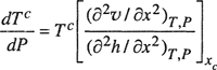
Equation (12-15) is not useful because it is difficult to measure the second derivatives of υ and h with respect to x. Further, both of these derivatives vanish at the critical point; therefore, Eq. (12-15) must be rewritten

(12-16)

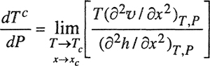
A large experimental effort must be made to evaluate the right side of Eq. (12-16); it would be easier to measure dT^c/dP directly. Nevertheless, Eq. (12-16) suggests an approximation, reasonable for simple mixtures, that allows us to use experimentally available quantities to estimate dT^c/dP. This approximation, suggested by Scott and coworkers (Myers et al, 1966), is a similarity hypothesis: we assume that υ and h, plotted against x, show similar shapes. That is, we assume that the molar excess volume υ^E and the molar excess enthalpy h^E depend on x and T according to

(12-17)

(12-18)

where F(x,T) is an arbitrary function of mole fraction x and temperature T. This assumption, substituted into Eq. (12-16), gives

(12-19)

where are the molar excess volume and the molar excess enthalpy at critical composition x_c and critical solution temperature T^c.

Because are not strongly sensitive to T and x (i.e., they do not show anomalous or “catastrophic” behavior at T^c and x_c), they can be estimated from dilatometric and calorimetric data in the critical region without direct measurements at the critical point.

Table 12-2 shows a test of Eq. (12-19). Experimental results for are compared with those for dT^c/dP. The test is limited to five systems where the required experimental data are available. Agreement is surprisingly good, even though these systems are far from simple mixtures.

Table 12-2 Predicted and measured effect of pressure on critical solution temperatures in binary systems (Myers et al., 1966; Clerke and Sengers, 1981).

Equation (12-16), a purely thermodynamic equation, is of no use by itself. However, when combined with physical insight, it produces the much more useful (approximate) Eq. (12-19).

In the preceding paragraphs we indicated how, under certain conditions, pressure may be used to induce immiscibility in liquid binary mixtures that, at normal pressures, are completely miscible. To conclude this section, we consider briefly how the introduction of a third component can bring about immiscibility in a binary mixture that is completely miscible in the absence of the third component. In particular, we are concerned with a binary liquid mixture where the added (third) component is a gas; in this case, elevated pressures are required to dissolve an appreciable amount of the added component in the binary liquid solvent. For the situation to be discussed, phase instability is not a consequence of the effect of pressure on the chemical potentials, as was the case in previous sections, but follows instead from the additional component that affects the chemical potentials of the components to be separated. High pressure enters into our discussion only indirectly, because we want to use a highly volatile substance for the additional component.

The situation under discussion is similar to the familiar salting-out effect in liquids where a salt, added to an aqueous solution, serves to precipitate one or more organic solutes. Here, however, instead of a salt, we add a gas; to dissolve an appreciable quantity of gas, the system must be at elevated pressure.

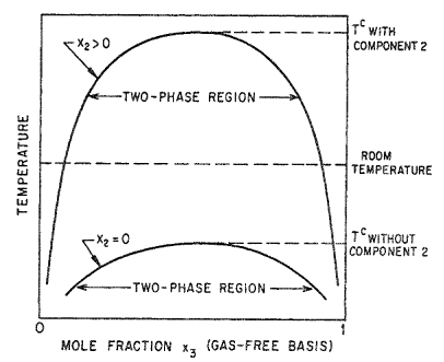
We consider a binary liquid mixture of components 1 and 3; to be consistent with previous notation, we reserve subscript 2 for the gaseous component. Components 1 and 3 are completely miscible at room temperature; the (upper) critical solution temperature T^c is far below room temperature, as indicated by the lower curve in Fig. 12-17. Suppose now that we dissolve a small amount of component 2 in the binary mixture; what happens to the critical solution temperature? This question was considered by Prigogine (1943), who assumed that for any binary pair that can be formed from the three components 1, 2, and 3, the excess Gibbs energy (symmetric convention) is

Figure 12-17 Effect of gaseous component (2) on mutual solubility of liquids (1) and (3).

(12-20)

where α_ij is an empirical (Margules) coefficient determined by the properties of the i-j binary. Prigogine has shown that, upon adding a small amount of component 2, the rate of change in critical temperature is given by

(12-21)

To induce the desired immiscibility in the 1-3 binary at room temperature, we want ∂T^c/∂x₂ to be positive and large.

Let us now focus attention on the common case where all three binaries exhibit positive deviations from Raoult’s law, i.e., α_ij > 0 for all i-j pairs. If T^c for the 1-3 binary is far below room temperature, then that binary is only moderately nonideal and α₁₃ is small. We must now choose a gas that forms a highly nonideal solution with one of the liquid components (say component 3) while it forms with the other component (component 1) a solution that is only modestly nonideal. In that event,

(12-22)

and

(12-23)

Equations (12-21), (12-22), and (12-23) indicate that under the conditions described, ∂T^c/∂x₂ is both large and positive, as desired; i.e., dissolution of a small amount of component 2 in the 1-3 mixture raises the critical solution temperature as shown in the upper curve of Fig. 12-17. From Prigogine’s analysis we conclude that if component 2 is properly chosen, it can induce binary miscible mixtures of components 1 and 3 to split at room temperature into two liquid phases having different compositions.

As shown by Balder (1966) thermodynamic considerations may be used to establish the phase diagram of a ternary system consisting of two miscible liquid components and a supercritical gas at high pressures. Such diagrams have been obtained experimentally (Elgin and Weinstock, 1959; Francis, 1963; Chappelear and Elgin, 1961) for a variety of ternary systems and have led to suggestions for separations using a high-pressure gas as the phase-splitting agent.

Gas-Gas Equilibria

Thermodynamic analysis of incomplete miscibility in liquid mixtures at high pressures [Eqs. (12-2), (12-3), and (12-4)] can also be applied to gaseous mixtures at high pressures. It has been known since the beginning of recorded history that not all liquids are completely miscible with one another, but only in the mid-twentieth century have we learned that gases may also, under suitable conditions, exhibit limited miscibility. The possible existence of two gaseous phases at equilibrium was predicted on theoretical grounds by van der Waals as early as 1894 and again by Onnes and Keesom (1907). Experimental verification, however, was not obtained until about 40 years later.

Immiscibility of gases is observed only at high pressures where gases are at liquid-like densities, as shown in Sec. 12.2. The term gas-gas equilibria is therefore misleading because it refers to fluids whose properties are similar to those of liquids, very different from those of gases under normal conditions. For our purposes here, we define two-component, gas-gas equilibria as the existence of two equilibrated, stable, fluid phases at a temperature in excess of the critical of either pure component; both phases are at the same pressure but have different compositions.

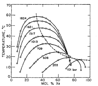
Figure 12-18 shows some experimental results for the helium/xenon system. As described in Sec. 12.2, the mixture helium/xenon is of type III and forms gas-gas equilibria of the first kind. At temperatures several degrees above the critical of xenon,¹⁰ the two phase compositions are significantly different, even at pressures as low as 200 bar. However, to obtain the same degree of separation at higher temperatures, much higher pressures are required.

¹⁰ The critical temperature of xenon is 16.6°C.

Figure 12-18 Gas-gas equilibria in the helium/xenon system (de Swaan Arons and Diepen, 1966).

A theoretical analysis of the helium/xenon system was reported by Zandbergen et al, (1967) who based their calculations on the Prigogine-Scott theory of corresponding states for mixtures (Prigogine, 1957; Scott, 1956). Zandbergen et al. use the three-liquid theory to obtain an expression for the volumes of helium/xenon mixtures as a function of temperature, pressure, and composition.

Different models were used by several authors (Kleintjens and Koningsveld, 1980; Trappeniers et al., 1971, 1974) to describe gas-gas immiscibility observed in other systems.

Equations of state provide a logical model for gas-gas equilibrium calculations. If a suitable equation of state is available for a mixture, it is possible to calculate critical lines for that mixture. That is, at least in principle, it is possible to compute phase diagrams such as those shown in Fig. 12-6. Pittion-Rossillon (1980), using an equation of state valid for hard-sphere mixtures combined with the attractive part of the van der Waals equation, predicted immiscibility in binary mixtures at high pressure, in good agreement with experimental data. Calculations were reported by Scott and van Konynenburg (1980) with the original van der Waals equation and by Deiters and coworkers with the Redlich-Kwong (Deiters and Pegg, 1989) or with the Carnahan-Starling-Redlich-Kwong (Kraska and Deiters, 1992) equations of state. Using conventional mixing rules, phase diagrams as in Fig. 12-6 can be qualitatively predicted. As expected, however, the original van der Waals equation is not sufficiently accurate to give quantitative agreement with experiment; however, it is sufficiently realistic to reproduce qualitatively most of the binary phase diagrams that have been observed.

Quantitative calculation of critical lines requires not only a good equation of state for mixtures, but also sophisticated computing techniques, as discussed, for example, by Stockfleth and Dohrn (1998), Michelsen (1980, 1981), Heidemann (1980), and Peng and Robinson (1977). The basis for these calculations is the theory of thermodynamic stability for multicomponent systems. A good introduction to that theory is given by Tester and Modell (1997) and by Prigogine and Defay (1954). We do not here discuss stability theory but, instead, show results for some simple cases.

Suppose we have a binary gaseous mixture containing components 1 and 2, such that critical temperature T_c2 is larger than T_c1. We now ask: At a temperature T, slightly larger than T_C2, does this mixture exhibit gas-gas equilibria? Following Temkin (1959), we assume that the properties of the mixture are given by the original van der Waals equation with constant b given by a linear function and constant a by a quadratic function of mole fraction. What conditions must be met by pure-component constants a and b and by binary constant a₁₂ to produce gas-gas equilibria? Temkin showed that gas-gas equilibria can exist, provided that

(12-24)

and that

(12-25)¹¹

¹¹ Taking into consideration the relations between van der Waals parameters a and b with the critical constants, Eqs. (12-24) and (12-25) can also be written as, and , respectively.

Because component 2 is the heavier component, Eq. (12-24) tells us that gas-gas equilibria near T_C2 are unlikely if there is a very large difference in molecular sizes, i.e., b₁ can be smaller than b₂ but not very much smaller. Equation (12-25) tells us that the attractive forces between unlike molecules (given by a₁₂) must be appreciably lower than those calculated by the arithmetic mean of a₁ and a₂. These conclusions are consistent with our intuitive ideas about mixtures. We can imagine that if we shake a box containing oranges and grapefruit [that satisfies Eq. (12-24)], the contents of that box might prefer to segregate into two separate regions, one rich in oranges and the other rich in grapefruit. However, if the box contains grapefruit and walnuts [that does not satisfy Eq. (12-24)], segregation is less likely because walnuts, unlike oranges, easily fit into the void regions of an assembly of grapefruit.

Equation (12-25) also is easy to understand. It says that for partial miscibility, the forces of attraction between unlike molecules must be weak; if molecules 1 and 2 do not like each other, they have little tendency to mix, but prefer to stay with neighbors identical to themselves.

If we assume that for nonpolar systems, a₁₂ = (a₁a₂)^1/2, Eq. (12-25) reduces to

(12-26)

In other words, the intermolecular force parameter a₁ must be less than about 5% of parameter a₂. This is a severe requirement. For example, if component 2 is carbon dioxide, then Eq. (12-26) is satisfied only by helium. For the binary helium/carbon dioxide, Eq. (12-24) is also satisfied and, indeed, gas-gas equilibria have been observed for that system at temperatures slightly above the critical for carbon dioxide.

12.4 Thermodynamic Analysis

Thermodynamic analysis has already been used in previous sections for deriving the equations for liquid-liquid and gas-gas equilibria. We return here to the same subject for a more general discussion.

As discussed in each of the previous chapters, the fundamental equilibrium relation for multicomponent, multiphase systems is most conveniently expressed in terms of fugacities: for any component i, the fugacity of i must be the same in all equilibrated phases. However, this equilibrium relation is of no use until we can relate the fugacity of a component to directly measurable properties. The essential task of phase-equilibrium thermodynamics is to describe the effects of temperature, pressure, and composition on the fugacity of each component in each phase of the system of interest. For any component i in a system containing m components, the total differential of the logarithm of the fugacity f_i is

(12-27)

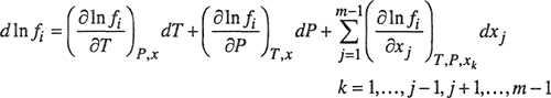
Thermodynamics gives limited information for each of the three coefficients that appear on the right-hand side of Eq. (12-27). The first term can be related to the partial molar enthalpy and the second to the partial molar volume; the third term can be related to the Gibbs energy and that, in turn, can be described by a solution model or an equation of state. For a complete description of phase behavior, we must say something about each of these three coefficients, for each component, in every phase. In high-pressure work, it is important to give particular attention to the second coefficient that tells us how phase behavior is affected by pressure.

When analyzing typical experimental data, it is often difficult to isolate the effect of pressure because, more often than not, a change in the pressure is accompanied by a simultaneous change in either the temperature or the composition, or both. A striking example of such simultaneous changes is given by experimental results in Fig. 12-19 that show the effect of pressure on the melting temperature of solid argon (Mullins and Ziegler, 1964). Line A gives the melting line for pure argon as reported by Clusius and Weigand (1940); the melting temperature rises with pressure, as predicted by the Clapeyron equation, because argon expands upon melting. Line B gives results of Mullins and Ziegler for the melting temperature of argon in the presence of high-pressure helium gas; these results are similar to those for pure argon, and again the melting temperature rises with increasing pressure. Finally, line C gives the melting temperature for argon in the presence of high-pressure hydrogen gas; Mullins and Ziegler also reported these data. We are struck and perhaps puzzled by the completely different behavior of line C: The melting temperature now falls with rising pressure.

Figure 12-19 Effect of pressure on melting temperature of argon. Qualitative difference between lines B and C is due to effect of composition on the liquid-phase fugacity of argon.

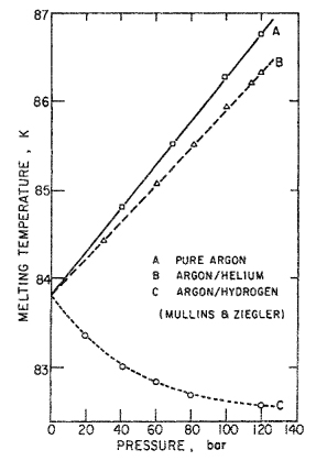
The qualitative difference between lines B and C can be clarified by thermodynamic analysis when we note that the three-phase equilibrium temperature is determined by two separate effects: first, the effect of pressure on the fugacities of solid and liquid argon is essentially the same for the three cases A, B, and C; and second, there is the effect of liquid composition on the fugacity of liquid argon. It is the effect of composition for case B that is much different from that for case C. At a given pressure, the solubility of hydrogen in liquid argon is much larger than that of helium; because pressure and composition simultaneously influence the fugacity of liquid argon, we find that the presence of hydrogen alters the equilibrium temperature in a manner qualitatively different from that found in the presence of helium. The fugacity of liquid argon is raised by pressure but lowered by solubility of another component. For helium (low solubility), the pressure effect dominates, but for hydrogen (high solubility), the effect of composition is more important. We shall not here go into a more detailed analysis of this particular system. We merely wish to emphasize that the fugacity of a component is determined by the three variables temperature, pressure, and composition; that in a typical experimental situation these influences operate in concert; and that whatever success we may expect in explaining the behavior of a multicomponent, multiphase system is determined directly by the extent of our knowledge of the three coefficients given in Eq. (12-27).

At present we know least about the first coefficient, rigorously related to enthalpy by

(12-28)¹²

¹² Equation (12-28) is the same as Eq. (6-3).

where is the partial molar enthalpy of i and the molar enthalpy of i in the ideal-gas state at the same temperature. While we would like to use information on to help us toward calculating f_i, we almost never can do so in high-pressure work because so little is known about enthalpies of fluid mixtures at high pressures. (In typical chemical engineering work, it is more common to reverse the procedure, i.e., to differentiate fugacity data with respect to temperature, to estimate enthalpies.) As a result, the best procedure for most cases is to analyze experimental phase-equilibrium data as a function of pressure and composition along an isotherm, and to allow any empirical parameters obtained from such analysis to vary with temperature as dictated by the experimental results.

While formal thermodynamic analysis is equally useful for predicting the effect of pressure, temperature, or composition on phase behavior, it is the effect of pressure that is often simplest to understand because it is directly related to volumetric data through the fundamental relation for molar Gibbs energy g

(12-29)

that, in turn, leads to

(12-30)

In Sec. 10.3 we briefly discussed the effect of pressure on the solubility of a sparingly soluble gas in a liquid. We here continue that discussion to show how thermodynamic analysis can predict unexpected phase behavior: When the solubility of a sparingly soluble gas is plotted against pressure, the plot may show a maximum.

To illustrate, consider the solubility of nitrogen in water at 18°C (Krichevsky and Kasarnovsky, 1935). Let subscript 2 stand for nitrogen. At equilibrium,

(12-31)

Taking logarithms and total differentials, Eq. (12-31) becomes

(12-32)

At constant temperature,

(12-33)

and

(12-34)

Because nitrogen is sparingly soluble in water at 18°C, Henry’s law holds; therefore, at constant temperature,

(12-35)

At 18°C, the volatility of water is very low: y₂ ≈ 1, and therefore the last term in Eq. (12-33) can be neglected.

Substituting Eqs. (12-33), (12-34) and (12-35) into Eq.(12-32), we obtain at constant temperature,

(12-36)

Because y₂ ≈ 1, we can set the vapor-phase partial molar volume of nitrogen equal to the molar volume of pure gaseous nitrogen, . Because solubility x₂ << 1, we can set

(12-37)

While is a strong function of pressure, is essentially independent of pressure in a solvent (here water) far below its critical temperature. Experimental data (Moors et al., 1985; Angus et al., 1979) for and are shown as a function of pressure in the lower part of Fig. 12-20. As indicated by Eq. (12-36), we expect a maximum in solubility x₂ when = .

Figure 12-20 Solubility of nitrogen in water at 18°C. Calculation of maximum solubility according to the Krichevsky-Kasarnovsky equation.

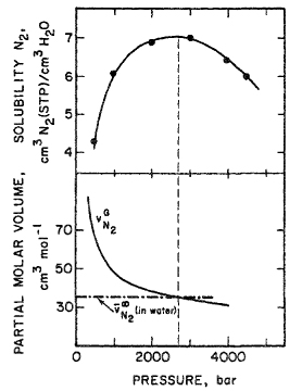
The upper part of Fig. 12-20 shows experimental solubility data (Basset and Dode, 1936) for nitrogen in water to high pressures. As predicted by Eq. (12-36) the observed solubility goes through a maximum near 2700 bar, consistent with experimental volumetric data.

Equation (12-30) indicates the important role of the partial molar volume in high-pressure phase equilibria. For mixtures of ordinary liquids remote from critical conditions, the partial molar volume of component i is often very close to the molar volume of pure liquid i at the same temperature; for such cases, in other words, Amagat’s law is a good assumption. However, for concentrated solutions of gases in liquids, the assumption is poor; at conditions approaching critical, it is very poor. Partial molar volumes may be positive or negative, and near critical conditions they are usually strong functions of the composition. For example, in the saturated liquid phase of the system carbon dioxide/n-butane at 71.1°C, for butane is 112.4 cm³ mol^-1 when the mole fraction of CO₂ is small, and it is -149.8 cm³ mol^-1 at critical composition, x_CO2 = 0.71.

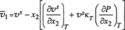
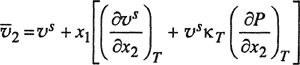
It is difficult to measure partial molar volumes and unfortunately many experimental studies of high-pressure vapor-liquid equilibria report no volumetric data at all; more often than not, experimental measurements are confined to total pressure, temperature, and phase compositions. Even in those rare cases where liquid densities are measured along the saturation curve, there is a fundamental difficulty in calculating partial molar volumes as indicated by the exact relations between partial molar volumes and isothermal saturated molar volume υ^s in a binary system:¹³

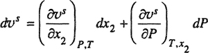
¹³ To derive Eq. (12-38) we must note that, at constant temperature, υ^s is a function of both x₂ and P:

(12-38)

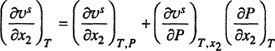
(12-39)

where compressibility κ_T is defined by

(12-38a)

Therefore,

(12-38b)

The partial molar volume is related to υ^s by

(12-38c)

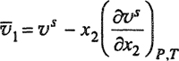
Simple substitution then gives Eq. (12-38).

(12-40)

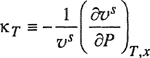
Experimental data for υ^s are sometimes available, but experimental compressibilities for mixtures are rare.

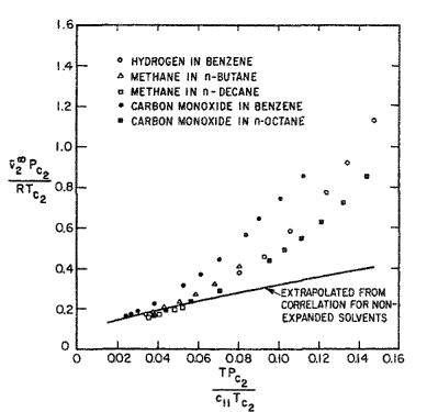
For dilute solutions, the literature contains some direct (dilatometric) measurements of , the partial molar volume of the more volatile component, but the accuracy of these measurements is usually not high. A survey by Lyckman et al. (1965) established the rough correlation shown in Fig. 12-21. On the ordinate, the partial molar volume is nondimensionalized with the critical temperature and pressure of component 2; the abscissa is also dimensionless and includes c₁₁, the cohesive-energy density of the solvent, component 1 (see Sec. 7.2). Figure 12-21 is useful for rough approximations in systems remote from critical conditions. For expanded solvents, i.e., for solvents at temperatures approaching T_c, the partial molar volume of the solute tends to be much larger than that suggested by the correlation as indicated in Fig. 12-22. Brelvi and O’Connell (1972) give an alternative correlation for

Figure 12-21 Partial molar volumes of gases in dilute liquid solutions.

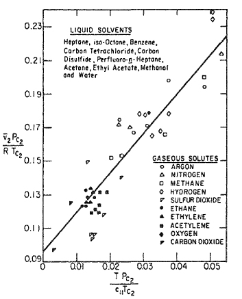
Figure 12-22 Partial molar volumes of gaseous solutes at infinite dilution in expanded solvents.

If we can write an equation of state for liquid mixtures, we can then calculate partial molar volumes directly by differentiation. For a pressure-explicit equation, the most convenient procedure is to use the exact relation

(12-41)

where V is the total volume of the mixture containing n₁ moles of component 1, etc.

12.5 Supercritical-Fluid Extraction

To illustrate the importance of partial molar volumes, we return to our previous discussion (Sec. 5.14) of the solubility of a solid in a compressed gas. This solubility can become surprisingly large when the compressed gas is near its critical point, leading to a separation operation called supercritical fluid extraction. We do not here go into details¹⁴ but show how the essence of supercritical fluid extraction is directly related to the partial molar volume of the solute in the compressed gas. Under certain conditions, this partial molar volume can be negative and extremely large, much larger than the molar volume of the pure solute.

¹⁴ See, e.g., McHugh and Krukonis (1994); E. Kiran and J. F. Brennecke (Eds., 1993), Supercritical Fluid Engineering Science, American Chemical Society Symposiom Series 514, Washington: ACS; T. J. Bruno and J. F. Ely (Eds., 1991), Supercritical Fluid Technology: Reviews in Modem Theory and Applications, Boston: CRC Press; K. P. Johnston and J. M. Penninger (Eds., 1989), Supercritical Fluid Science and Technology, American Chemical Society Symposium Series 406, Washington: ACS.

Consider the solubility of a heavy component (2) in a dense gas (1) at temperature T and pressure P. For simplicity, let component 2 be a solid such that the solubility of component 1 in the solid phase is negligible. The equation of equilibrium is

(12-42)

where y is the mole fraction in the vapor phase and φ is the vapor-phase fugacity coefficient.

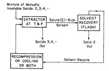
At gas-phase densities approaching the critical, solubility y₂ is sensitive to small changes in T and P because, in the critical region, these have a large effect on the gas-phase density. This sensitivity has applications in separation technology (supercritical extraction)¹⁵, where solvent recovery is an important economic consideration. Figure 12-23 shows a schematic diagram of a particularly simple supercritical-extraction separation process. Suppose that component 2 is in a mixture of mutually insoluble solids; suppose also that dense gas 1 (the solvent) selectively dissolves solid 2 at T and P close to the critical of the solvent. After the solute-saturated solvent is removed, it is slightly expanded (or heated, or both), significantly reducing the solvent’s density. That reduction lowers y₂; solid 2 precipitates and the solute-lean solvent is recycled to the extraction unit after recompression (or cooling, or both). The advantage of this separation process is that, under favorable circumstances, energy requirements for solvent recovery may be lower than those required for a conventional extraction process, using liquid solvents.¹⁶

¹⁵ Supercritical fluid solvents also provide unique reaction media because of the strong pressure dependence of their densities and solvent properties (such as viscosity, mass transfer coefficients, etc.). This strong pressure dependence offers the capability of controlling solvent properties, reaction rates, and selectivities through easily conducted pressure regulation.

¹⁶ While the discussion here is limited to a mixture of mutually insoluble solids, supercritical extraction can also be applied to condensed mixtures of soluble (or partially soluble) solids or liquids. The principles are the same, but molecular-thermodynamic analysis is now more complex because, in addition to pure-component, condensed-phase fugacities, we require first, condensed-phase activity coefficients, and second, solubilities for the gaseous solvent if the condensed phase is a liquid. For a review, see M. E. Paulaitis, V. J. Krukonis, and R. C. Reid, 1983, Rev. Chem. Eng., 1: 179.

Extractions with supercritical fluids are potentially useful in many industries, in particular for extraction of bioactive substances from natural products (for a review, see King, 1993 and Rizvi, 1994). In general, an extract obtained by supercritical extraction from natural products is a mixture of various bioactive substances (such as isomers and substituted derivatives). For example, to isolate coumarin (known for its

Figure 12-23 Idealized application of supercritical extraction. Temperature T and pressure Pare slightly above the solvent’s critical. In the recovery step, a small drop in P (or small rise in 7) significantly lowers the solubility of solid 2 in the gaseous solvent. (In this idealized example, the solvent is totally selective for solid 2.)

strong antibiotic and anticoagulation properties) for pharmaceutical use by extraction with supercritical CO₂ from a natural plant, the extract also contains appreciable amounts of isomers and numerous coumarin derivatives (Yoo, 1997; Choi, 1998). The design of a supercritical fluid process requires the solubilities of each component in the supercritical fluid. Figure 12-24 compares solubilities at 308.15 K of coumarin and its methoxy-group and hydroxy-group derivatives in supercritical CO₂. As Fig 12-24 shows, coumarin exhibits the highest solubility in CO₂; its solubility is about two orders of magnitude higher than those of its derivatives. This large solubility difference is required for the feasibility of any supercritical-fluid-based extraction process.

Figure 12-24 Solubility of coumarin, 7-methoxycoumarin and 7-hydroxycoumarin in supercritical CO₂ at 308.15 K (Yoo et al., 1997). Lines are best fit of experimental data.

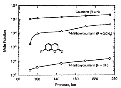
Figure 12-25 presents an illustration of a practical application of supercritical fluid solvents in the oleochemical industry. This figure shows distribution coefficients (K factors) of oleic acid and triolein (a major component of vegetable oils, such as rapeseed and olive oil) in supercritical carbon dioxide at 40°C (Bharath et al., 1992). Carbon dioxide is a convenient solvent for supercritical extraction. Among others, it has the advantage of allowing extractions at temperatures close to room temperature (the CO₂ critical temperature is 31.1°C), particularly useful for thermally labile natural materials such as polyunsaturated fatty acids like oleic acid. A major advantage of CO₂ derives from its environmentally-friendly properties: it is not toxic; it does not burn or explode; it is easily vented into the atmosphere; and it is inexpensive.

Figure 12-25 K factors (Bharath et al., 1992) as a function of pressure (for feeds of 50 weight % and 70 weight % of triolein, CO₂-free basis) for oleic acid (—) and triolein (- - - -) obtained from vapor-liquid-equilibrium data with supercritical CO₂ at 40°C.

Figure 12-25 shows that the distribution coefficients of both oleic acid and triolein vary with pressure and with feed composition. However, K for oleic acid is ten times larger than that of triolein, suggesting that extraction with supercritical CO₂ can provide an alternative (Gonçalves et al., 1991) to conventional fractionation processes such as solvent extraction (where, typically, toxic organic solvents are used) and low-pressure distillation (that requires relatively high temperatures).

Another area of rapidly developing possibilities for supercritical fluid technology is in various aspects of environmental control (Abraham and Sunol, 1997) such as removal of pesticides (e.g., DDT and pyrethrin), polyaromatic hydrocarbons, polychlorinated aromatic compounds (PCB’s), dioxins, etc. from contaminated soils.

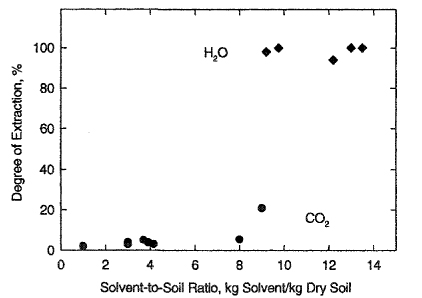
Technologies have been developed for extraction of organic compounds from aqueous and solid environmental matrices. The attractive feature of this process is the ease of separation of the extracted solute from the supercritical fluid that results in the creation of smaller waste volumes of the now concentrated organic, improving the efficiency of subsequent waste-treatment processes such as incineration. Figure 12-26 shows results of supercritical removal of hydrocarbons from soil contaminated with 5 weight % of long-chain alkanes, 4 weight % of monoaromatic, and 2 weight % of polyaromatic hydrocarbons (Firus et al., 1997). Figure 12-26 shows that supercritical water (at 653 K and 25 MPa) removes virtually all the contaminants from the soil. However, supercritical CO₂ (at 353 K and 20 MPa) achieves no more than 21% of extraction (even with large solvent-to-soil ratio), because of the lower operating temperature.

Figure 12-26 Extraction of hydrocarbons from soil with supercritical CO₂ and H₂O as a function of solvent-to-soil ratio. : H₂O at 653 K and 25 MPa; : CO₂ at 353 K and 20 MPa. The critical temperature of CO₂ is 304 K and that of water is 647 K.

In modeling the phase behavior (e.g. an equation of state) of natural products such as those indicated in Figs. 12-24 and 12-25, there is an additional difficulty: due to the complex nature of most natural products, basic physical properties (such as critical data), and constants (such as Antoine vapor-pressure constants), are not available. They are usually estimated from semi-empirical methods such as those described by Reid et at. (1987) and Lyman et al. (1990).

When component 2 is much heavier than component 1, at temperatures and pressures slightly above the critical of solvent 1, fugacity coefficient φ₂ almost always very small compared to unity. As indicated by Eq. (12-42), when pressure and temperature are held constant, solubility y₂ is inversely proportional to φ₂. The advantage of supercritical extraction follows from the sensitivity of φ₂ to pressure (and, to a lesser extent, temperature) when the solvent’s density is near its critical.

Experimental results have shown that, near the solvent’s critical state, φ₂ << 1, yielding a solubility y₂ much larger than that calculated assuming ideal-gas behavior. Experimental results also show that, near the solvent’s critical state, a small decrease in pressure produces a large rise in φ₂; it is this observation that facilitates solvent recovery.

The effect of pressure P on fugacity coefficient φ₂ is directly related to the partial molar volume :

(12-43)

When y₂ << 1, and when T and P are near the critical of the solvent, is large and negative. To illustrate, let component 2 be naphthalene and let component 1 be carbon dioxide. (The critical temperature of carbon dioxide is 31.1°C; the critical pressure is 73.8 bar.) To calculate from a pressure-explicit equation of state, we use Eq. (12-41).

Partial molar volumes for naphthalene in carbon dioxide have been calculated using Chueh’s modification (Chueh and Prausnitz, 1967) of the Redlich-Kwong equation of state. Results are shown in Fig. 12-27. Because the vapor pressure of solid naphthalene is very small in the range 35 to 50°C, y₂ is also small compared to unity; therefore, the calculated results in Fig. 12-25 are for solutions infinitely dilute in naphthalene (y₂ = 0). The calculations were performed using conventional mixing rules (quadratic in mole fraction for a and linear in mole fraction for b) with binary parameter k₁₂ = 0.0626 as determined from solubility data. Vapor-phase densities for pure carbon dioxide were obtained from the IUPAC tables (Angus et al., 1976).

Figure 12-27 Partial molar volumes of naphthalene infinitely dilute in compressed carbon dioxide. Partial molar volumes are large and negative in the critical region.

Figure 12-27 shows that, at constant temperature, is negative and goes through a sharp minimum when plotted against pressure, in agreement with the data of van Wasen (1980). Further, is extremely large, especially at 35°C and (about) 78 bar. At this temperature, the calculated minimum in is -10.8 L mol^-1; for comparison, the critical volume of pure carbon dioxide is +0.0944 L mol^-1.

Figure 12-27 and Eq. (12-43) indicate that at pressures near 78 bar and at 35°C, a small decrease in pressure very much raises φ2 thereby very much reducing solubility y₂. The sharp change in φ2 with pressure is the basis of efficient solute recovery in supercritical fluid extraction.

12.6 Calculation of High-Pressure Vapor-Liquid Equilibria

If a liquid mixture at temperature T is in equilibrium with a vapor at high pressure, it is usually necessary that one of the components must be supercritical; that is, the mixture is likely to contain at least one component i whose critical temperature T_ci > T. This follows because the vapor pressures of most liquids are not large (critical pressures of typical pure liquids are in the range 30 to 100 bar) and therefore, with few exceptions, high-pressure vapor-liquid equilibria as found in nature and in the chemical industry apply to mixtures with at least one subcritical component and at least one supercritical component.

The thermodynamics of high-pressure vapor-liquid equilibria is, in principle, similar to that of the solubility of gases in liquids, as discussed in Chap. 10. However, the concepts of Chap. 10 are generally not useful for our purposes here because we are now concerned with a wide range of liquid-phase concentrations, not only with dilute solutions.

It is possible analytically to represent high-pressure vapor-liquid equilibria using, for the liquid phase, the common thermodynamic functions: Henry’s constant, activity coefficient and partial molar volume. But experience has shown that in typical cases, these functions are not useful, especially for multicomponent mixtures. A more successful route for quantitatively describing high-pressure vapor-liquid equilibria is provided by the fugacity coefficient, applied to both phases, as indicated in Sec. 3.6.

Consider a binary liquid mixture with mole fractions x₁ and x₂ at temperature T and pressure P; in equilibrium with this liquid mixture is a vapor with mole fractions y₁ and y₂. The equations of equilibrium are

(12-44)

and

(12-45)

where f is the fugacity and φ is the fugacity coefficient. The equilibrium ratios (K factors) are given by

(12-46)

(12-47)

12.7 Phase Equilibria from Equations of State

To calculate fugacity coefficients, we can use a partition function (see App. B) or, what is equivalent for our purposes here, an equation of state. Equation-of-state methods provide one of the most useful techniques used in chemical engineering practice for modeling phase equilibria of multicomponent systems.¹⁷

¹⁷ For a review see A. Anderko, 1990, Fluid Phase Equilibria, 6:145.

In the equation-of-state method, a single equation of state is used to represent all fluid phases; for vapor-liquid equilibria, the equation is assumed to be valid for both the vapor-phase mixture and the liquid-phase mixture.

For each component i in the vapor phase,

(12-48)

as discussed in Chap. 3. Here n_i is the number of moles of component i and n_T is the total number ofmoles in the vapor phase. Similarly, for each component i in the liquid phase

(12-49)

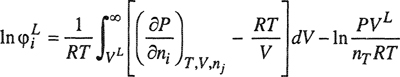
where n_i and n_T now refer to the liquid phase.

To use Eqs. (12-48) and (12-49), we require a suitable equation of state that holds for the entire range of possible mole fractions x and y at system temperature T and for the density range between 0 and This last condition is necessary because the integral in Eq. (12-49) goes from the ideal-gas state (infinite volume) to the saturated-liquid density. At present, there are no satisfactory equations of state that meet these requirements with generality. However, for many mixtures, we have reasonable, approximate equations of state that provide useful results.

The simplest procedure for using Eqs. (12-48) and (12-49) is to choose an equation of state that holds for pure fluid 1 and for pure fluid 2 and to assume that this same equation of state holds for all mixtures of 1 and 2 by interpolation. To fix ideas, consider, for example, Soave’s (1972) modification of the Redlich-Kwong equation:

(12-50)

where a(T) depends on temperature according to

(12-51)

(12-52)

where, for normal fluids,

(12-53)¹⁸

¹⁸ Soave (1993, Fluid Phase Equilibria, 84; 339) proposed another expression for the temperature dependence of the attractive parameter of the Soave-Redlich-Kwong equation. This function is a two-parameter extension of the original form and can be applied to polar and nonpolar fluids. The new expression (valid to ω = 0.5) is:

For nonpolar or slightly polar fluids, m = 0.484 + 1.515ω - 0.044ω² and n = 2.756 m - 0.700. For strongly polar fluids, m and n must be fitted from experimental data.

for acentric factors 0 < ω < 0.5.

Constant b is given by

(12-54)

as in the Redlich-Kwong equation.

Now comes the important step: extension of Eq. (12-50) to the binary mixture. The simplest procedure (but by no means the only possible procedure) is to assume a one-fluid theory of mixtures, that is, to assume that the equation of state for the mixture is the same as that for a hypothetical “pure” fluid whose characteristic constants b and a(T) depend on composition.

One-fluid theory assumes that for the mixture we can generalize Eq. (12-50), i.e. to assume that it holds for the mixtures for both phases. The remaining task is to specify how b and a(T) depend on composition (mixing rules).

The common procedure is to write mixing rules that are quadratic in mole fraction. For a binary mixture,

(12-55)

(12-56)

where is either x or y.

Constants b_ii and a_ii(T) refer to the pure-component values; however, b_l2 and a₁₂(T) are binary parameters. It is convenient to express these in the form

(12-57)¹⁹

¹⁹ If c₁₂ = 0, Eq. (12-55) reduces to the linear form

(12-58)

where the absolute values of binary parameters |c₁₂| and |k₁₂| are small compared to unity. For simple mixtures of nonpolar components, it is customary to set c₁₂ = 0 and to fit k_l2 to binary vapor-liquid equilibrium composition data.²⁰ For simple systems, k_l2 is often nearly independent of temperature. While k₁₂ and c₁₂ may depend on temperature, they cannot depend on pressure or density without thereby substantially increasing the complexity of the resulting equation for the fugacity coefficient.

²⁰ For mixtures that are highly asymmetric with respect to size (for example, hydrogen/anthracene), it is sometimes better to adjust c₁₂ to experimental data while setting k₁₂ = 0. See, for example, A. I. ElTwaty and J. M. Praosnitz, 1980,Chem. Eng. Sci., 35: 1765.

For calculating high-pressure vapor-liquid equilibria from an equation of state, the computational procedure is not trivial. In a typical case for a binary mixture, the given quantities may be P and x₁ (and x₂). Equations (12-44), (12-45), (12-48), and (12-49) must then be used to find T, y_l (and y₂). However, to use Eqs. (12-48) and (12-49), we must know the molar volumes v^v and v^L To find these, we use the equation of state for the mixture[say, Eq. (12-50)] twice, once for the vapor mixture and once for the liquid mixture.

For the binary case under consideration here, there are four unknowns: y, T, v^V and V^L. To find these, it is necessary to solve simultaneously four independent equations. These are Eqs. (12-44) and (12-45) [with Eqs. (12-48) and (12-49) substituted for the fugacity coefficients] and Eq. (12-50) twice, once for each phase. A similar procedure is used for multicomponent mixtures. Numerical techniques for such calculations are described in numerous references [see, e.g., Anderson (1980, 1980a) and Michelsen (1980); there are many others].

To illustrate this method for calculating high-pressure vapor-liquid equilibria, Fig. 12-28 shows results for the system methane/propane. Calculations are based on Soave’s modification of the Redlich-Kwong equation of state with mixing rules given by Eqs. (12-55) and (12-56). In these calculations c₁₂ = 0. Good agreement with experiment is obtained when k₁₂ = 0.029. A small change in k_l2 can significantly affect the calculated results.

Figure 12-28 Isothermal pressure-composition diagram for methane/propane. Calculations using Redlich-Kwong-Soave equation of state. Experimental data from Reamer et al. (1950).

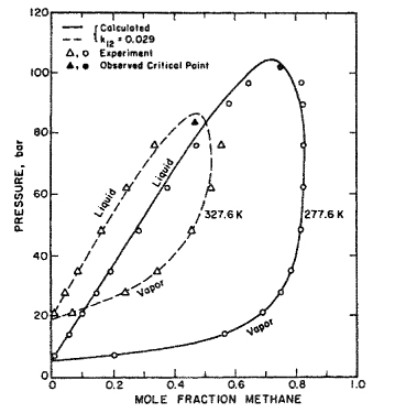
Figure 12-29 shows calculated K factors for nitrogen/propylene, using C ₁₂= 0 and k _l2= 0.0915. Again, agreement with experiment is good.

Another illustration is given in Fig. 12-30 for the system hydrogen sulfide/water. In this case c₁₂ = 0.08 and k₁₂ = 0.163. Pure-component constants were found from Eqs. (12-51) to (12-54), even though Eq. (12-53) is obtained from vapor-pressure data for paraffins. The high value of k_l2 is not surprising because the geometric-mean approximation [Eq. (12-58) is poor for aqueous mixtures. For this system it is likely that the binary constants (especially k₁₂) depend significantly on temperature.

Calculations similar to these can be made with any one of a large number of equations of the van der Waals form. Many such calculations have been reported, notably by Peng and Robinson (1976), Ishikawa et al. (1980), and Dohrn and Brunner (1995). While most work has been limited to binary systems, extension to ternary (or higher) systems is straightforward. If such extension uses mixing rules that are quadratic in mole fraction [Eqs. (12-55) and (12-56)], only pure-component and binary parameters are required.

Figure 12-29 Calculated and observed (Graus0 et al., 1977) K factors for nitrogen/propyiene. Caiculations using Red!ich-Kwong-Soave equation of state.

Figure 12-30 Experimental (Selieck eta!., 1952) and calculated (Eveiein etal., 1976) phase equilibria for the system hydrogen sulfide/water at 171 °C.

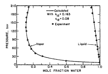
To calculate vapor-liquid phase equilibria for a binary system, pure-component constants are rarely sufficient; for reliable results it is necessary to use also at least one binary parameter that, with few exceptions, cannot be estimated with sufficient accuracy from unicomponent data alone. However, to calculate vapor-liquid phase equilibria for a ternary (or higher) system, ternary (or higher) parameters are often not required for reliable results. In many cases, ternary (or higher) vapor-liquid equilibria can be predicted using only pure-component and binary parameters.

To illustrate, Fig. 12-31 shows vapor-liquid equilibria obtained by Sandier and coworkers at 410.9 K for the ternary system N₂/CO₂/cyclohexane, as well as for the constituent binaries N₂/c-C₆H₁₂ and CO₂/c-C₆H₁₂. According to the phase rule, a ternary mixture with two phases in equilibrium has 3 degrees of freedom; these are described by volumes (see Table 12-1) in P-T- space. Therefore, a convenient two-dimensional way of representing ternary phase equilibrium data is by using an isothermal pressure-composition²¹ (or isobaric temperature-composition) prism with a triangle as a base. Each of the four cross-sectional triangles is an isothermal-isobaric phase diagram, and each side of the prism corresponds to the appropriate binary P-x diagrams, as illustrated in Fig. 12-31. At 410.9 K, both N₂ and CO₂ are supercritical and therefore this binary is not shown in Fig. 12-31.

²¹ Using an isothermal (or isobaric) representation, the degrees of freedom are reduced by one. Using an isothermal and isobaric representation, the degrees of freedom are reduced by two.

In addition to experimental data, Fig. 12-31 shows also calculations using the Peng-Robinson equation of state:

(12-59)

For a pure fluid, constant b is given by

(12-60)

while a(T), a function of temperature, is given by

(12-61)

(12-62)

(12-63)

Here, T_c is the critical temperature and β depends on acentric factor ω according to β = 0.37464 + 1.54226 ω - 0.26992 ω² (for 0 ≤ ω ≤ 0.5).

Figure 12-31 Vapor-liquid equilibria for the system N ₂/CO₂/c-C6 H₁₂ at 410.9 K. The four triangles shown on top are isothermal-isobaric phase diagrams for the ternary mixture at 410.9 K and at the pressures indicated. At bottom, phase diagrams of the constituent binaries CO₂/c-C₆H₁₂ and N₂/c C₆H₁₂ (also at 410.9 K) and their relation to the 68.9-bar triangular diagram. Experiment;— Calculated from Peng-Robinson equation with the binary parameters listed in Table 12-3. (Shibata and Sandier, 1989).

Using the conventional mixing rales for a mixture [Eqs. (12-55) and (12-56)], the fugacity coefficient for component k in a mixture is given by

(12-64)

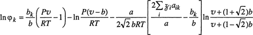
where _i is the mole fraction of component i.

The phase behavior of the ternary N₂/CO₂/c-C₆H₁₂ system was predicted using the binary parameters k_ij given in Table 12-3, determined from binary data only (for the binary N₂/CO₂, k ₁₂ was set to zero).

Table 12-3 Binary parameters k _ij[Eq. (12-58)] in the Peng-Robinson equation as obtained from binary data at 410.9 K.

Figure 12-31 shows good agreement between experimental and calculated results obtained for the ternary N₂/CO₂/c-C₆H₁₂ at 410.9 K and at 68.9, 137.9, 206.8, and 275.7 bar, and also for the binaries N₂/c-C6 H₁₂ and CO₂/c-C₆H₁₂ at the same temperature. However, near the critical region agreement between calculated and experimental results is not satisfactory. When calculations are based on an equation of state of the van der Waals form (e.g., Redlich-Kwong-Soave, Peng-Robinson), it is often found that the calculated two-phase region is larger than that given by experiment, as shown in Fig. 12-31. While we now have a good understanding of why equations of state of the van der Waals form fail in the critical region, it is not a simple matter to “fix” these equations for better performance. In the critical region, density fluctuations contribute strongly to thermodynamic properties. These fluctuations, ignored in van der Waals-type equations of state, can be taken into account but the procedure for doing so is complex.²²

²² L. Lue and J. M. Prausnitz, 1998, AlChE J., 44: 1455; Z. Y. Cheng, M. A. Anisimov, J. V. Sengers, 1997, Fluid Phase Equilibria, 128: 67.

Non-Quadratic Mixing Rules

To extend pure-fluid equations of state to mixtures of nonpolar (or slightly polar) components, it is customary to use classical one-fluid mixing rules, as proposed by vander Waals. In the one-fluid theory, it is assumed that the properties of a fluid mixture are identical to those of a hypothetical pure fluid, at the same temperature and pressure, whose equation-of-state parameters are functions of mole fraction. In the van der Waals approximation, these functions are quadratic in mole fraction.

For highly nonideal mixtures, however, quadratic mixing rules are inadequate. Several methods have been proposed to modify the original mixing rules. In many cases the modified mixing rules include composition-dependent or density-dependent binary interaction parameters. Density-dependent mixing rules are formulated to obtain a correct representation of mixture properties at both high and low-density regions: in the limit of low density, they reproduce the correct composition dependence of the mixture second virial coefficient (a quadratic function in mole fraction, as shown in Sec. 5.3), whereas in the high-density limit (or infinite pressure), mixing rules are determined to force agreement with some excess-Gibbs-energy model for a liquid mixture (see, for example, Dimitrelis and Prausnitz, 1990). Some authors have suggested mixing rules independent of density, as suggested by excess-Gibbs-energy models. Most of these mixing rules, however, violate the theoretically-based boundary condition that the second virial coefficient must be quadratic in mole fraction.

Promising mixing rules are those proposed by Wong et al. (1992, 1992a; Sandier et al., 1994).²³ Their rules produce the correct low-density limit (the mixture second virial coefficient has a quadratic dependence in mole fraction) and a high-density limit consistent with experiment (the equation of state predicts the same excess molar Helrnholtz energy at infinite pressure, , as a function of composition as that obtained from a selected activity-coefficient model). Wong-Sandier mixing rules are not density dependent.

²³ For a description of the capabilities and limitations of the Wong-Sandier mixing rule see P. Coutsikos et al., 1995, Fluid Phase Equilibria, 108: 59, and M. A. Satyro and M. A. Trebble, 1996, ibid., 115: 135.

The Wong-Sandier model is applied to a van der Waals-type equation of state with

(12-65)

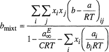
and

(12-66)

where C is a constant dependent on the equation of state. For the Peng-Robinson equation, for the van der Waals equation, C = -1.

The composition-independent cross second virial coefficient [b -(a/(RT)]_ij, obtained from the equation of state, is related to those of the pure components by

(12-67)

where k_ij is a binary interaction parameter for the second virial coefficient. This interaction parameter is usually obtained from fitting experimental vapor-liquid data as expressed by the molar excess Gibbs energy g^E as a function of mole fraction x at constant temperature. To fix K_ij, it is common to use g^E at x = 0.5.

For the high-density limit, Wong and Sandier equate the excess Helmholtz energy at infinite pressure obtained from the equation of state to that obtained from a chosen liquid-phase activity-coefficient model (van Laar or NRTL, etc.), using the approximation

where (T, x_i) is the molar excess Helmholtz energy for a fixed composition x_i and temperature T in the infinite-pressure limit. In subsequent calculations, it is common practice to neglect the effect of temperature on

Figure 12-32 compares measured and calculated vapor-liquid equilibria for the binary 2-propanol/water (Wong et al., 1992a). The calculations were performed with the Peng-Robinson equation of state - with pure component parameters obtained from the correlation of Stryjek and Vera (1986) - using the mixing rules of Wong-Sandier (as described above) with determined from the van Laar equation. The van Laar parameters were obtained by correlating experimental vapor-liquid-equilibrium data at 4.12 bar, reported in the DECHEMA data series (Gmehling and Onken, 1977); binary interaction parameter k₁₂ = 0.326 was determined by adjusting the excess Gibbs energy calculated from the equation of state (at 4.12 bar) to that calculated from the van Laar model. This parameter was then used to predict the phase behavior at other pressures and temperatures. As Fig. 12-32 shows, with the parameters obtained at conditions where all components are subcritical, this model can predict well vapor-liquid equilibria at conditions where one of the components (2-propanol) becomes supercritical.

Figure 12-32 High-pressure vapor-liquid equilibria for the binary 2-propartoI/water. Calculations from the Peng-Robinson equation, as modified by Stryjek and Vera (1986) using the Wong-Sandier mixing rules (1992) with k₁₂ = 0.326. —Calculated; ο Experiment (Barr-David and Dodge, 1959).

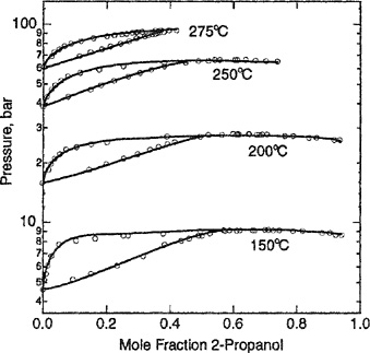
The main attraction of the Wong-Sandier mixing method follows from its ability to extrapolate vapor-liquid-equilibrium data to other (usually higher) temperatures and pressures.

12.8 Phase Equilibria from a Corresponding-States Correlation

Corresponding-states correlations can be used to calculate fugacities of components in mixtures of normal (nonpolar or slightly polar) fluids; these fugacities are then used to compute phase equilibria. The general procedure is first, to write a reduced equation of state for compressibility factor z:

(12-68)

or a reduced equation of state of the form

(12-69)

where T_c, P_c, and U_c, are critical temperature, pressure, and volume and where X is some additional characteristic parameter such as the acentric factor.²⁴ Functions F_Z or F_p may be analytic, tabular or graphical; for computer applications, analytical functions are most convenient.²⁵ From Eq. (12-72) or (12-73), we calculate fugacity coefficients as discussed in Chap. 3 [Eqs. (3-14) and (3-53)].

²⁴ For a fixed value of acentric factor (see Sec. 4.13), υ_c is not an independent parameter when T_c and P_c are specified.

²⁵ Analytical equations are given by D. R. Schreiber and K. S. Pitzer, 1989, Fluid Phase Equilibria, 46: 113.

To extend Eqs. (12-68) or (12-69) to mixtures, we use the pseudocritical hypothesis. The essential step here is to assume some expressions (mixing rules) indicating how the characteristic properties (T_c, X, P_c or υ_c depend on composition. We then find the fugacity coefficient for a component z in the mixture by differentiation; for a binary mixture, fugacity coefficient φ₁ is found from

(12-70)

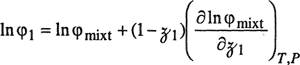
where is the mole fraction in either the liquid phase or the vapor phase. The condition of vapor-liquid equilibrium is given by Eqs. (12-44) and (12-45).

The literature presents many examples where corresponding-states correlations have been used to calculate vapor-liquid equilibria at high pressures. One of the most successful is the correlation given by Mollerup (1980) for mixtures of natural gases (methane, nitrogen, ethane, propane, and carbon dioxide). Mollerup uses these mixing rules for the critical temperature, critical volume, and acentric factor:

(12-71)

(12-72)

(12-73)

with

(12-74)

(12-75)

where k_ij is a binary parameter characteristic of the i-j interaction. Because calculated results are sensitive to k_ij Mollerup has taken much care to find the best values from reliable binary experimental data. Figure 12-33 shows K factors for the methane/propane system calculated by Mollerup. For this simple system, Mollerup obtains excellent agreement with experiment for a wide temperature range.

Figure 12-33 K factors for the methane/propane system calculated by Mollerup using corresponding-states theory.

Another example of how corresponding states may be used to calculate high-pressure vapor-liquid equilibria is provided by Plöcker’s extension (Plöcker et al, 1978) to mixtures of the correlation for pure fluids presented by Lee and Kesler (1975) (see Sec. 4.11). Plöcker’s chief interest is in asymmetric mixtures, i.e., in mixtures of normal fluids differing appreciably in molecular size. For such mixtures, Plöcker²⁶ found good agreement with experiment upon modifying Eq. (12-75) to read

²⁶ A description similar to that of Plöcker is presented by Plazer and Maurer, 1993, Fluid Phase Equilibria, 84: 79, and tested successfully for a iarge number of systems.

(12-76)

The exponent 1/4 provides an empirical attempt to take into account (crudely) that when a small molecule interacts with a large molecule, the small molecule “sees” only part of the large molecule. Weighting intermolecular attractions as in Eq. (12-71), emphasizes molecular size too strongly; on the other hand, if the exponent 1/4 were replaced by exponent zero, no weight at all would be given to molecular size.

Plöcker also rewrites Eq. (12-75) in the equivalent form

(12-77)

where K_ij = 1 - k_ij.

Figure 12-34 illustrates calculations from Plöcker and coworkers using the correlation of Lee and Kesler. The same authors present a large number of binary parameters _ij. For binaries where limited experimental information is available, they correlated K_ij parameters as a function of the dimensionless group (T_ci U_ci)/(T_ci U_ci).

Figure 12-34 Calculated (Plöcker et a!., 1978) and experimental (Robinson and Besserer, 1972) K factors for the binary system hydrogen sulfide/isobutane.

Other applications of corresponding states to high-pressure phase equilibria include the shape-factor method of Leland and coworkers (Leach et al., 1968).

12.9 Vapor-Liquid Equilibria from the Perturbed-Hard-Chain Theory

The perturbed-hard chain (PHC) theory, discussed in Sec. 7.16, can be used to calculate vapor-liquid equilibria at high pressures. As shown by Liu et al. (1980), it is particularly useful for mixtures containing large and small molecules (e.g., ethylene and polyethylene) at high pressures. We describe briefly some simplified models based on PHC theory. Section 12.10 presents a model for fluids with associating molecules.

Kim et al. (1982) use the Carnahan-Starling expression for hard-sphere molecular repulsion [Eq. (7-238)] but for the attractive part they use an expression based on the local-composition model of Lee et al. (1985); the resulting equation of state has a relatively simple mathematical form. The attractive contribution is

(12-78)

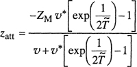
where Z_M is the maximum lattice-site coordination number. For the R = 1.5 square-well fluid potential (see Sec. 5.5), Kim et al. used the lattice model of Lee with Z_M = 18. For mixtures, Kim used also mixing rules based on van der Waals one-fluid theory. Figures 12-35 and 12-36 show examples of calculations using this simplified form of the PHC theory.

Figure 12-35 Calculated (simplified PHC theory of Kim) and experimental K factors for n-hexane in the ethane/n-hexane binary at 450.0, 394.3, and 338.7 K (Kim et al., 1986).

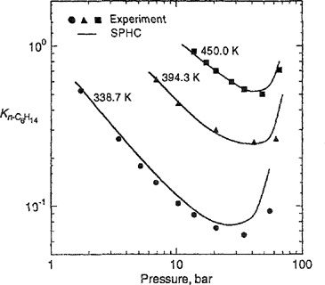
Figure 12-35 compares calculated with experimental K factors for the ethane/n-hexane system at three temperatures. Predictions of the simplified PCH theory are in good agreement with experiment. The K factors shown in Fig. 12-35 were calculated using only pure-component parameters (T^*, U^* and c); in this fortuitous case, no adjustable binary interaction parameters are required. However, as Fig. 12-36 shows, to describe vapor-liquid equilibria for mixtures of ethane with a heavy n-alkane²⁷ (eicosane, K-C₂₀H₄₂) at 350 K, it is necessary to use a binary parameter k₁₂²⁸ obtained from data regression of the phase envelopes at 350 K (Peters et al., 1988). Using pure-component parameters only (k₁₂ = 0), fair agreement with the experiment (better than 5% in pressure) is obtained. With k₁₂ obtained at 350 K, the simplified PHC theory represents well the experimental data at 450 K. For comparison, Fig. 12-36 shows also calculated results from the Redlich-Kwong-Soave equation of state for the same binary at 450 K, but with k₁₂ optimized at this temperature.

²⁷ In these calculations, pure-component data were obtained by linearly extrapolating plots of Kim’s parameters versus carbon number. Parameter Z_M has been set equal to 36.

²⁸ As usual, binary interaction parameter k₁₂ is defined by ε₁₂ = (ε₁₁ε₂₂)^1/2(1-k₁₂) where e is an energy parameter.

Figure 12-36 Vapor-liquid equilibria for ethane/eicosane at 350.0 K and 450.0 K (Peters et al., 1988). (a) At 350.0 K: o Experiment;…. Simplified PHC, k₁₂ = 0;—Simplified PHC, k₁₂ = 0.020; (b) At 450.0 K: o Experiment; Simplified PHC, k₁₂ = 0.020; Redlich-Kwong-Soave, k₁₂ = -0.0077.

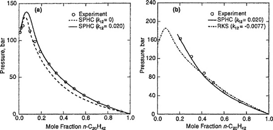
In a manner similar to that used by van Konynenburg and Scott with the van der Waals equation of state, and Deiters with the Redlich-Kwong equation (Deiters and Pegg, 1989) and with the Carnahan-Starling-Redlich-Kwong equation (Kraska and Deiters, 1992), van Pelt et al. (1991) used the simplified PHC equation to calculate semi-quantitative critical curves and phase behavior of binary fluid mixtures. In addition to the six types described in Fig. 12-6, van Pelt found new types of phase behavior.

Extensive application of PHC is discussed by Cotterman (1986). To illustrate, Fig. 12-37 shows calculated and observed solubilities (Henry’s constants) for five solutes in low-density polyethylene and Fig. 12-38 shows calculated and observed K factors for a 12-component synthetic oil at 322 K with 70 mol % carbon dioxide. The oil contains nitrogen and hydrocarbons from methane to tetradecane.

Figure 12-37 Weight-fraction Henry’s constants for some solutes in low-density polyethylene. Symbols are experimental data (o Liu, 1976; • Maloney, 1976); —— PHC (Cotterman, 1986) with one binary parameter k₁₂ per binary system.

Figure 12-38 K factors for 12-component synthetic oil with 70 mol % carbon dioxide at 322 K. Symbols : Experiment (Turek et al., 1984); PHC (Cotterman, 1986) with one binary parameter k₁₂ per binary system.

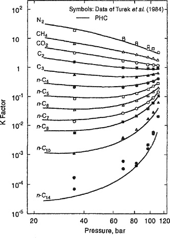
Additional extensions of PHC theory are reported by Donohue and coworkers (Ikonomou and Donohue, 1986, 1988; Donohue and Vimalchand, 1988; Elliot et al, 1990), who give special attention to the effect of polarity and hydrogen bonding.

The literature is rich with variations of PHC theory (or the similar chain-ofrotators equation of Chao and coworkers (Chien et al., 1983). Each one has advantages and disadvantages but, essentially, all give, more or less, similar results. The key to success is to use a good binary parameter that must be fitted to experimental binary data.

12.10 Phase Equilibria Using the Chemical Theory

A classical method to describe strongly nonideal and associating (hydrogen-bonding) mixtures, is provided by coupling an equation of state with a chemical theory of association and solvation, as indicated in Sec. 5.10. An example of this method is the model of Gmehling based on PHC theory.

Gmehling et al. (1979)²⁹ truncated the perturbation expansion at the second-order term, reducing the original 21 universal A_nm constants required by Eq. (7-224) to 10 without significant loss of accuracy. They also extended the PHC theory to mixtures containing one (or more) strongly polar component by including chemical dimerization equilibria. The extension takes polar forces into account by assuming that, in addition to the nonideal properties given by the PHC equation of state, strong polar forces can form dimers. Thus, a binary mixture of A and B is considered to be a five-species mixture containing monomers A and B and, in addition, dimers A2, B9, and AB. The concentrations of these five species are calculated by material balances and by chemical equilibria:

²⁹ See also Grenzheuser and Gmehling (1986).

(12-79)

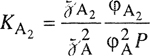
(12-80)

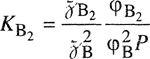
(12-81)

where represents mole fraction. The equilibrium constants are functions only of temperature. For a binary mixture, fugacity coefficients φ are calculated from the (five-species) partition function. Equilibrium constants and can be determined from pure-component properties, K_AB must be obtained from binary data. If only A is strongly polar, = K_AB = 0.

Figure 12-39 shows calculated and observed equilibria for methanol/water. Gmehling reduced the number of adjustable binary parameters by making some reasonable simplifying assumptions. The results shown in Fig. 12-39 require only two binary parameters for the indicated ranges of temperature, pressure, and composition.

Figure 12-39 Vapor-liquid equilibria for methanol/water (Gmehling et al., 1979).

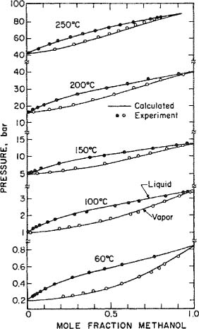
Gmehling’s model considers only monomers and dimers; trimers (and higher aggregates) are neglected. The advantage of considering only dimers is that extension to mixtures is straightforward. As shown in the following paragraphs, it is possible to construct a consistent theory that includes trimers, tetramers, etc. but then extension to mixtures is difficult.

In the “chemical” theory of mixtures, molecules may associate or solvate to form new species; chemical equilibria are included in the equation of state. Thermodynamic properties of polar fluids and their mixtures follow from chemical equilibria leading to associated or solvated species and from physical (nonspecific) interactions between all species present in the solution. The chemical effects, taken into account by a molecular-based association model, are combined with the physical effects into one comprehensive equation of state.

To illustrate, we consider a simple but representative model presented by Heidemann and Prausnitz (1976). This model combines an equation of the van der Waals form with a continuous linear association model. Here a pure fluid is considered to be a mixture of monomers, dimers, trimers, etc. In the definition of reduced density, η = n_Tb/v the total number of moles n_T is not a constant but depends on the density and temperature. Also, van der Waals parameter b depends on the true composition of the fluid; in the low-density limit b = πN_A σ^3/6 (where all molecules are monomers) where N_A is Avogadro’s constant and σ is the collision diameter.³⁰

³⁰ In the classical van der Waals equation of state, b is four times larger than the b defined in Heidemann’s work.

The equation of state is separated into its repulsive and attractive contributions,

(12-82)

The repulsive term is rewritten in terms of the compressibility factor z_rep′

(12-83)

where V is the total volume.

The attractive-force contribution in the equation of state is rewritten in the form

(12-84)

where π_att is a function only of reduced density η Constant â depends on the composition of the mixture (monomers, dimers, trimers, etc.); in the low-density limit (all molecules are monomers), constant â is that of the conventional van der Waals-type equation.

Based on experimental evidence indicating that molecular clusters exist for polar and hydrogen-bonded molecules, Heidemann postulates a linear association model where a monomer molecule X₁ can associate to form dimers, trimers, etc., according to the chemical equilibria

(12-85)

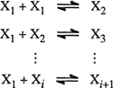
To apply the equation of state to mixtures, the classical mixing rules are

(12-86)

(12-87)

where _i (_i = n_i/n_T) is the mole fraction of species i (monomer, dimer, etc.) in the mixture, and a and b refer to the monomer.

To simplify the model, Heidemann introduce also the following reasonable assumptions

(12-88)

(12-89)

where a and b refer to the monomer.

Conservation of mass relations require that the total number of moles n_T is related to n₀, the number of moles that would exist if there were no association, by

(12-90)

Combination of Eq. (12-90) with Eqs. (12-86) to (12-89) gives

(12-91)

and

(12-92)

With the results presented above, we obtain for the equation of state,

(12-93)

In Eq. (12-93), z_rep and π_att are functions only of reduced density η).

To obtain the ratio n_T/n₀³¹ we define the chemical equilibrium constant (a function of temperature only),

³¹ The ratio n_T/n₀ is a measure of the extent of association. In the absence of association, n_T/n₀ is unity, whereas for strongly associating species n_T/n₀ is always less than unity except at veiy low pressures, where this ratio goes to unity.

(12-94)

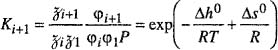
where φ is the fugacity coefficient, obtained from the equation of state [using e.g. Eq. (3-53)], Δh⁰ is the standard enthalpy of association, and Δs⁰ is the standard entropy of association [see Eq. (5-111)].

Heidemann considers equilibrium constants K independent of the degree of association, i.e., K₂ = K₃ =… = K. From material balance equations we find n_T/n₀,

(12-95)

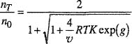
Upon substitution in Eq. (12-93), we obtain the equation of state for associating fluids

(12-96)

with

(12-97)

In Eq. (12-96), υ is the volume per mole of non-associated molecules, that is, υ = V/n₀. In the limit as K → 0 (no association), Eq. (12-96) reduces to the equation for nonassociating fluids, as expected. Moreover, we can use in Eq. (12-96) any desired explicit form for z_rep, e.g. the Carnahan-Starling equation of state gives g = (4η – 3η²)/(1 – η)². For π_att we could use e.g. the Redlich-Kwong equation of state: π_att = η²/(1+ 4η).

Heidemann’s continuous linear association model briefly described above provides an efficient method for describing phase equilibria of pure highly polar and associating fluids. However, useful extension to mixtures containing two or more associated fluids is not simple without severe simplifying assumptions.

Using the equation of state of Yu and Lu (1987), Heidemann’s formalism was extended to mixtures containing one associated and one or more unassociated fluids by Anderko (1989; 1989a). Many other association models have been proposed, notably by Anderko (1990) and by Economou et al. (1991, 1992), but all of them are essentially similar to that of Heidemann.

Consider, as an example, the method proposed by Lencka and Anderko (1993) applied to the calculation of vapor-liquid equilibria for the system hydrogen fluoride/C₂F₃Cl₃ (Freon-113). This system is of technical interest because HF is a byproduct in the production of a common refrigerant.³² Anderko assumes that the compressibility factor of an associated mixture is separated into a physical (van der Waals-type) and a chemical (association) contribution,

³² While chlorine-containing freon refrigerants are now in decline because of environmental considerations (decomposition of ozone), production of environmentally acceptable refrigerants may also produce HF as a side product.

(12-98)

In Eq. (12-98), contribution z_phys is expressed by a common equation of state for the true monomeric species and z_chem is defined as the ratio of the total number of moles of all species to the number that would be present in the absence of association (n₀); that is, z_chem = n_T/n₀

For Z_phys Anderko uses the Peng-Robinson equation of state. To obtain an expression for z_chem, Anderko considers that, in the mixture, HF can form linear multimers formed by consecutive self-association reactions,

Anderko does not assume that the chemical equilibrium constant is independent of j. Instead, he uses a distribution function f(j):

(12-99)

K_j,j+1 = f(j)K

where K is a constant. Distribution function f(j) depends on the nature of the associating fluid. Assuming that f(1) = 1, then K is the dimerization constant. The equilibrium constant K_i for the i-merization reaction

is related to the consecutive association constants [Eq. (12-99)] by

(12-100)

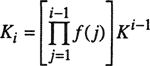
On the basis of simulation data for hydrogen fluoride, Lencka and Anderko proposed that distribution function f(j) should smoothly cover a small range of j values with a maximum near j = 6, as shown in Fig. 12-40.

Figure 12-40 Distribution function f(j) proposed by Lencka and Anderko (1993) for hydrogen fluoride. The distribution function shows a maximum near j = 6 indicating that HF preferentially forms hexamers.

Anderko obtained his distribution function by fitting the equation of state to isothermal pure HF thermophysical data; the equation above then give z_chem. Figure 12-41 shows calculated vapor-liquid-liquid equilibria for the system HF/C₂F₃Cl₃ at 383.15 K. Anderko’s model represents well the experimental data for this strongly nonideal system. Using no binary parameters, Anderko’s model gives a good, nearly quantitative prediction. However, agreement is improved when a small adjustable binary parameter is introduced.

Figure 12-41 Vapor-liquid-liquid equilibria for HF/C₂F₃Cl₃ at 383.15 K (Lencka and Anderko, 1993). • Experiment; — Association model of Anderko (with k₁₂ = -0.01); - - - - Association mode! of Anderko (with K₁₂ = 0).

In this binary case, only one of the components (HF) forms dimers, trimers, etc.; the other component (C₂F₃Cl₃) does not. Drastic additional simplifying assumptions are required to extend Anderko’s model to a binary where both components form dimers, trimers, etc. as well as cross-dimers, cross-trimers, etc.

12.11 Summary

When binary fluid mixtures are subjected to high pressure, a large variety of phase behavior is possible. Many binary systems have been studied experimentally, giving rise to numerous types of phase diagrams; some of these are shown in the early sections of this chapter. When we go to ternary (or higher) fluid mixtures, the possible variety of phase behavior increases further, but for such mixtures experimental data are scarce.

Analysis of high-pressure phase diagrams shows that, at some conditions, retrograde phenomena can occur. Such phenomena are commonly found in petroleum and natural-gas reservoirs: at some conditions, contrary to intuition, isothermal compression produces vaporization rather than condensation. For a thermodynamic description of high-pressure phase equilibria, the key thermodynamic equation is the pressure derivative of the chemical potential or fugacity; that derivative is directly related to the partial molar volume. If the partial molar volume is positive, an increase in pressure raises the fugacity. In an isothermal two-phase system, if we increase the pressure, we affect the distribution of a dilute component i between the two phases. As pressure rises, component i is shifted toward that phase where its partial molar volume is lower. Raising pressure increases the fugacity (escaping tendency) of i; as pressure rises, component i’s tendency to escape is larger in the phase where i has the larger partial molar volume.

Interpretation of high-pressure phase-equilibrium data is often not simple because (especially in binary systems) a change in pressure is usually accompanied by a simultaneous change in another intensive property. For example, in isothermal vapor-liquid equilibria for say, methane-toluene, if we raise the pressure, we not only change the densities but also the compositions of both phases. In a two-phase system, it is there-fore not possible experimentally to study the effect of pressure alone while keeping the compositions of both phases constant. However, the effect of pressure can be isolated from the effects of other intensive variables through thermodynamic analysis where we consider separately the effects of pressure, composition and temperature on the chemical potential (or fugacity) through the use of partial derivatives.

For a heavy solute i dilute in a light gas near that gas’ critical point, the partial molar volume of i is typically large and negative. Under these conditions, it follows that the fugacity coefficient of i is very much smaller than unity and, therefore, the solubility of i in the gas is much larger than that at conditions remote from the gas’ critical point. The large negative partial molar volume of the solute provides the thermodynamic basis for supercritical extraction processes; such processes enable separation of low-volatile compounds, e.g., biologically active substances in plants or pollutants in soil. Solvent recovery from the extract is simple because the solubility of the solute is highly sensitive to small changes in solvent density; a small decline in pressure precipitates the dissolved solute.

For describing isothermal liquid-liquid equilibria, we need expressions for the excess Gibbs energy and for the excess volume, both as functions of composition. Depending on the sign of the excess volume (positive or negative), rising pressure may induce phase splitting in a liquid mixture that is homogeneous at normal pressure or, vice versa, rising pressure may homogenize a liquid mixture that is heterogeneous at normal pressure.

For high-pressure vapor-liquid calculations, we need an equation of state that can describe the properties of both phases. In typical applications, we use an equation of state of the van der Waals form coupled with the one-fluid assumption: the configurational properties of a fluid mixture are assumed to be the same as those of a hypothetical pure fluid whose characteristic constants (a, b) are some composition average. The procedure for averaging is given by (mostly) empirical mixing rules. Many mixing rules have been proposed but there is no clear conclusion to indicate that any one mixing rule is the best. To obtain good agreement with experiment, details in a reasonable mixing rule are usually less important than the number and reliability of the adjustable binary parameters that appear in the mixing rule.

When strong polarity or chemical association are significant (e.g., carboxylic acids, alcohols, hydrogen fluoride), it is necessary to superimpose on the “physical” equation of state the contribution of “chemical” forces. The major contribution of chemical effects on thermodynamic properties follows from a change in the number of particles; for example, for dimerization, two particles join to become one particle giving a decrease in entropy. The extent of association due to chemical equilibria depends not only on temperature and pressure but also on concentration, often strongly so. As a result, when “chemical” forces are significant, complex phase behavior is often observed.

The fundamental thermodynamic relations that govern high-pressure phase equilibria are well understood. But these relations cannot be reduced to practice without good molecular-thermodynamic models. Good models are scarce, especially for application to regions both near to and far from critical conditions. Progress in molecular simulations is likely to improve our understanding of fluids and fluid mixtures under a variety of conditions, including high pressures. For practical application, the challenge will be to translate that understanding toward establishing reasonably simple, yet sufficiently accurate models for performing reliable, engineering-oriented calculations.

References

Abraham, M. A. and A. K. Sunol, (Eds.), 1997, Supercritical Fluids: Extraction and Pollution Prevention. Washington: ACS.

Anderko, A., 1989, Fluid Phase Equilibria, 45: 39.

Anderko, A., 1989a, Chem. Eng. Sci, 44: 713.

Anderko, A., 1990, Fluid Phase Equilibria, 61: 145.

Anderson, T. F. and J. M. Prausnitz, 1980, Ind. Eng. Chem. Process Des. Dev., 19: 1.

Anderson, T. F. and J. M. Prausnitz, 1980a, Ind. Eng. Chem. Process Des. Dev., 19: 9.

Angus, S., B. Armstrong, and K. M. de Reuck, (Eds.), 1976, IUPAC - International Thermodynamic Tables of the Fluid State – Carbon Dioxide. Oxford: Pergamon Press.

Angus, S., B. Armstrong, and K. M. de Reuck, (Eds.), 1979, IUPAC - International Thermodynamic Tables of the Fluid State – Nitrogen. Oxford: Pergamon Press.

Balder, J. R. and J. M. Prausnitz, 1966, Ind. Eng. Chem. Fundam., 5: 449.

Barr-David, F. and B. F. Dodge, 1959, J. Chem. Eng. Data, 4: 107.

Basset, J. and M. Dode, 1936, C. R. Acad. Sci. (Paris), 20: 775.

Becker, P. J. and G. M. Schneider, 1993, J. Chem. Thermodynamics, 25: 795.

Bharath, R., H. Inomata, T. Adschiri, and K. Arai, 1992, Fluid Phase Equilibria, 81: 307.

Bijl, H., Th. W. de Loos, and R. N. Lichtenthaler, 1983, Fluid Phase Equilibria, 14: 157.

Brelvi, S. W. and J. P. O’Connell, 1972, AIChE J., 18: 1239.

Brunner, E., 1985, J. Chem. Thermodynamics, 17: 985.

Chappelear, D. C. and J. C. Elgin, 1961, J. Chem. Eng. Data, 6: 415.

Chien, C. H., R. A. Greenkorn, K. C. Chao, 1983, AIChE J., 29: 560.

Choi, E. S., M. J. Noh, and K.-P. Yoo, 1998, J. Chem. Eng. Data, 43: 6.

Chueh, P. L. and J. M. Prausnitz, 1967, Ind. Eng. Chem. Fundam., 6: 492.

Clerke, E. A. and J. V. Sengers, 1981, Proc. 8^th Symp. Thermophys. Properties Am. Soc. Mech. Eng., New York.

Clusius, K. and K. Weigand, 1940, Z. Phys. Chem., B46: 1.

Connolly, J. F., 1966, J. Chem. Eng. Data, 11: 13.

Cotterman, R. L. and J. M. Prausnitz, 1986, AIChE J., 32: 1799.

Dahlmann, U. and G. M. Schneider, 1989, J. Chem. Thermodynamics, 21: 997.

De Loos, Th. W., L. J. de Graaf, and J. de Swaan Arons, 1996, Fluid Phase Equilibria, 117: 40.

De Swaan Arons, J. and T. W. de Loos, 1994, Phase Behavior: Phenomena. Significance, and Models. In Models for Thermodynamic and Phase Equilibria Calculations, (S. I. Sandler, Ed.). New York: Marcel Dekker.

Deiters, U.K. and I. L Pegg, 1989, J.Chem. Phys., 90: 6632.

Dimitrelis, D. and J. M. Prausnitz, 1990, Chem. Eng. Sci., 45: 1503.

Dohm, R. and G. Brunner, 1995, Fluid Phase Equilibria, 106: 213.

Donohue, M.D. and P. Vimalchand, 1988, Fluid Phase Equilibria, 40: 185.

Economou, I. G. and M. D. Donohue, 1991, AIChE J., 37: 1875.

Economou, I. G. and M. D. Donohue, 1992, Ind. Eng. Chem. Res., 31: 1203.

Elgin, J. C. and J. J. Weinstock, 1959, J. Chem. Eng. Data, 4: 3.

Elliot, J. R., S. J. Suresh, and M. D. Donohue, 1990, Ind. Eng. Chem. Res., 29: 1476.

Evelein, K. A., R. G. Moore, and R. A. Heidemann, 1976, Ind. Eng. Chem. Proc. Des. Dev., 15: 423.

Francis, A. W., 1963, Liquid-Liquid Equilibria. New York: Wiley-Intersdence.

Gmehling, J. and U. Onken, 1977, Vapor-Liquid Equilibrium Data Compilation: DECHEMA Data Series. Frankfurt: DECHEMA.

Gmehling, J., D. D. Liu and J. M. Prausnitz, 1979, Chem. Eng. Sci, 34: 951.

Gonçalves, M., A. M. P. Vasconcelos, E. Gomes de Azevedo, H. J. Chaaves das Neves, and M. Nunes da Ponte, 1991, J. Am. Oil Chem. Soc., 68: 474.

Gonikberg, M. G., 1963, Chemical Equilibria and Reaction Rates at High Pressures (trans, from Russian). Washington: Office of Technical Services, U.S. Dept. of Commerce.

Grausø, L., Aa. Fredenslund, and J. Mollerup, 1977, Fluid Phase Equilibria, 1: 13.

Gregorowicz, J., Th. W. de Loos, and J. de Swaan Arons, 1993, Fluid Phase Equilibria, 84: 225.

Grenzheuser, P. and J. Gmehling, 1986, Fluid Phase Equilibria, 25: 1.

Grzanna, R. and G. M. Schneider, 1996, Z. Phys. Chem., 193: 41.

Heidemann, R. A. and J. M. Prausnitz, 1976, Proc. Nat. Acad. Sci., 73: 1773.

Heidemann, R. A. and A. M. Khalil, 1980, AIChE J., 26: 769.

Hicks, C. P. and C. L. Young, 1975, Chem. Rev., 75: 119.

Ikonomou, G. D. and M. D. Donohue, 1986, AIChE J., 32: 1716.

Ikonomou, G. D. and M. D. Donohue, 1988, Fluid Phase Equilibria, 39: 129.

Ishikawa, T., W. K. Chung, and B. Lu, 1980, AIChE J., 26: 372.

Jeschke, P. and G. M. Schneider, 1982, J. Chem. Thermodynamics, 14: 547.

Kim, C.-H., P. Vimalchand, M. D. Donohue, and S. I. Sandler, 1986, AIChE J., 32: 1726.

King., M. B. and T. R. Bott (Eds.), 1993, Extraction of Natural Products Using Near-Critical Solvents. London: Chapman & Hall.

Kleintjens, L. A. and R. Koningsveld, 1980, J. Electrochem. Soc., 127: 2352.

Kraska, T. and U. K. Deiters, 1992, J. Chem. Phys., 96: 539.

Krichevsky, I. R. and J. S. Kasarnovsky, 1935, J. Am. Chem. Soc., 57: 2168.

Leach, J. W., P. S. Chappelear, and T. W. Leland, 1968, AIChE J., 14: 568.

Lee, B. I. and M. G. Kesler, 1975, AIChE J., 21: 510.

Lee, K.-H., M. Lombardo, and S. I. Sandler, 1985, Fluid Phase Equilibria, 21: 177.

Lencka, M. and A. Anderko, 1993, AIChE J., 39: 533.

Liu, D. D. and J. M. Prausnitz, 1976, Ind. Eng. Chem. Fundam., 15: 330.

Liu, D. D. and J. M. Prausnitz, 1980, Ind. Eng. Chem. Process Des. Dev., 19: 205.

Lyckman, E. W., C. A. Eckert, and J. M. Prausnitz, 1965, Chem. Eng. Sci, 20: 685.

Lyman, W. J., W. F. Reehl, and D. H. Rosenblatt, 1990, Handbook of Chemical Property Estimation Methods. Washington: ACS.

Maloney, D. P. and J. M. Prausnitz, 1976, AIChE J., 22: 74.

McHugh, M. A. and V. J. Krakonis, 1994, Supercritical-Fluid Extraction: Principles and Practice, 2^nd Ed. Boston: Butterworth-Heinemann.

Mehta, V. S. and G. Thodos, 1965, J. Chem. Eng. Data, 10: 211.

Michelsen, M. L., 1980, Fluid Phase Equilibria, 4: 1.

Michelsen, M. L. and R. A. Heidemann, 1981, AIChE J., 27: 521.

Mollerup, J., 1980, Fluid Phase Equilibria, 4:11.

Moors, J. C., R. Battino, T. R. Rettich, Y. P. Handa, and E. Wilhelm, 1982, J. Chem. Eng. Data, 27: 221.

Mullins, J. C. and W. T. Ziegler, 1964, Int. Ad. Cryog. Eng., 10: 171.

Myers, D. B., R. A. Smith, J. Katz, and R. L. Scott, 1966, J. Phys. Chem., 70: 3341.

Ochel, H., H. Becker, K. Maag, and G. M. Schneider, 1993, J. Chem. Thermodynamics, 25: 667.

Onnes, H. K. and W. H. Keesom, 1907, Commun. Phys. Lab. Univ. Leiden, Suppl. 16.

Peng, D.-Y. and D. B. Robinson, 1976, Ind. Eng. Chem. Fundam., 15: 59.

Peng, D.-Y. and D. B. Robinson, 1911, AIChE J., 23: 137.

Peters, C. J., J. L. de Swaan Arons, J. M. H. Levelt-Sengers, and J. S. Gallagher, 1988, AIChE J., 34: 834.

Pittion-Rossillon, G., 1980, J. Chem. Phys., 73: 3398.

Plöcker, U., H. Knapp, and J. M. Prausnitz, 1978, Ind. Eng. Chem. Process Des. Dev., 17: 324.

Poppe, G., 1935, Bull. Soc. Chim. Belg., 44: 640.

Prigogine, I, 1943, Bull. Soc. Chim. Belg., 52: 115.

Prigogine, I. and R. Defay, 1954, Chemical Thermodynamics. London: Longmans & Green.

Prigogine, I., 1957, The Molecular Theory of Solutions. Amsterdam: North-Holland.

Reamer, H. H., B. H. Sage, and W. N. Lacey, 1950, Ind. Eng. Chem., 42: 534.

Reid., R. C., J. M. Prausnitz, and B. E. Poling, 1987, The Properties of Gases and Liquids, 4^th Ed. New York: McGraw-Hill.

Rizvi, S. S. (Ed.), 1994, Supercritical Fluid Processing of Foods and Biomaterials. London: Blackie Academic and Professional Co.

Robinson, D. B. and G. J. Besserer, 1972, Nat. Gas Process. Assoc. Res. Report, 7.

Roozeboom, H. W., 1918, Die Heterogenen Gleichgewichte, Braunschweig.

Rowlinson, J. S. and F. L. Swinton, 1982, Liquids and Liquid Mixtures, 3^rd Ed. London: Butterworths.

Sadus, R. J., 1992, High Pressure Phase Behaviour of Multicomponent Fluid Mixtures. Amsterdam: Elsevier.

Sadus, R. J, 1994, AIChE J., 40: 1376.

Sage, B. H. and W. N. Lacey, 1938, Ind Eng. Chem., 30: 1299.

Sandler, S. I., H. Orbey, and B.-I. Lee, 1994. In Models for Thermodynamic and Phase Equilibria Calculations, (S. I. Sandler, Ed.), Chap. 2. New York: Marcel Dekker.

Schneider, G. M., 1966, Ber. Bunsenges. Phys. Chem., 70: 497.

Schneider, G. M., 1976, Pure Appl. Chem., 47: 277.

Schneider, G. M., 1978, In Chemical Thermodynamics, Specialist Periodical Report, (M. L. McGlashan, Ed.), Vol. 2, page 105. London: Chemical Society.

Schneider, G. M., 1993, Pure Appl. Chem., 65: 173.

Schouten, J. A., 1992, Physics Reports, 172: 33.

Scott, R. L., 1956, J. Chem. Phys., 25: 193.

Selleck, F. T., L. T. Carmichael, and B. H. Sage, 1952, Ind. Eng. Chem., 44: 2219.

Shibata, S. and S. I. Sandler, 1989, J. Chem. Eng. Data, 34: 419.

Soave, G., 1972, Chem. Eng. Sci., 27: 1197.

Specovius, J., M. A. Leiva, R. L. Scott, and C. M. Knobler, 1981, J. Phys. Chem., 85: 2313.

Stockfleth, R. and R. Dohm, 1998, Fluid Phase Equilibria, 145: 43.

Stryjek, R. and J. H. Vera, 1986, Can. J. Chem. Eng., 64: 323.

Temkin, M. I., 1959, Russ. J. Phys. Chem., 33: 275.

Tester, J. W. and M. Modell, 1997, Thermodynamics and Its Applications, 3^rd Ed. Englewood Cliffs: Prentice-Hall.

Timmermans, J., 1923, J. Chim. Phys., 20: 491.

Trappeniers, N. J., J. A. Schouten, and C. A. ten Seldam, 1971, Chem. Phys. Lett, 5: 541.

Trappeniers, N. J., J. A. Schouten, and C. A. ten Seldam, 1974, Physica, 73: 556.

Turek, E. A., R. S. Metcalfe, L. Yarborough, and R. L. Robinson, Jr., 1984, Soc. Pel. Eng. J., 24: 308.

Van Konynenburg, P. H. and R. L. Scott, 1980, Philos. Trans. R. Soc., 298: 495.

Van Pelt, A., C. J. Peters, and J. de Swaan Arons, 1991, J. Chem. Phys., 95: 7569.

Van Wasen, V. and G. M. Schneider, 1980, J. Phys. Chem., 84: 229.

Wallbruch, A. and G. M. Schneider, 1995, J. Chem. Thermodynamics, 27: 377. See also Errata, 1997, J. Chem. Thermodynamics, 29: 929.

Winnick, J., 1963, Dissertation, University of Oklahoma.

Winnick, J. and J. E. Powers, l966, AIChE J., 12: 460, 466.

Wong, D. S and S. I. Sandler, 1992, AIChE J., 38: 671.

Wong, D. S, H. Orbey, and S. I. Sandler, 1992a, Ind. Eng. Chem. Res., 31: 2033.

Yoo, K.-P., Shin, H. Y., M. J. Noh, and S. S. You, 1997, Korean J. Chem. Eng., 14: 341.

Yu, J. M. and B. C.-Y. Lu, 1987, Fluid Phase Equilibria, 34: 1.

Zandbergen, P., H. F. P. Knaap, and J. J. M. Beenakker, 1967, Physica, 33: 379.

Zeck, S. and H. Knapp, 1986, Fluid Phase Equilibria, 26: 37.

Problems

1. A typical P-T projection for water/n-alkane systems is presented below.

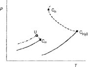
In the above figure, C_n and C_H2o are, respectively, the critical points of the n-alkane and of the water; U is the critical-end point of liquid-liquid-gas equilibrium; C_b is the binary homogeneous point (i.e. the point where the two-phase region separates into two parts); solid lines indicate pure-component saturation vapor pressures; dashed lines indicate binary mixture critical lines; and the dashed-dot line indicates three-phase liquid-liquid-gas equilibrium. Sketch P-x diagrams for the temperatures:

(i) T < T_U; (ii) T = T_U; (iii) T_U < T < T_Cn; (iv) T_Cn < T < T_Cb; (v) T = T_Cb; (vi) T_Cb < T < T_CH2O; (vii) T > T_CH2O.

2. Consider the following type II phase diagram:

(a) Draw the P-x projection for temperature T₁

(b) Draw T-x projections for pressures P₁ < P_UCEP, P₂ = P_UCEP, and P₃ > P_UCEP.

3. An alcohol is distributed between two immiscible fluids, hexane and dimethyl sulfoxide. Calculate the distribution coefficient of the alcohol between the two liquid phases (when the alcohol concentration is very small) at 30°C and 100 bar. The following binary data are available, all at 0°C and 1 bar pressure:

In your notation, use ’ for the hexane phase and ” for the dimethyl sulfoxide phase. State all assumptions made. Distribution coefficient K is defined as

where subscript A refers to alcohol.

4. At the normal melting point (5.5°C) the density of liquid benzene is 0.891 g cm^-3 and that of solid benzene is 1.010 g cm^-3. Find the melting temperature of benzene under a pressure of 200 bar.

The following vapor-pressure equations are available:

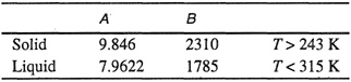
5. Consider an equimolar liquid mixture of components A and B at 300 K with a molar volume of 116.6 cm³ mol^-1. Using the Redlich-Kwong equation of state and the data given below, calculate the total pressure.

Henry’s constant for A infinitely dilute in B at 300 K is 7.01 bar. The molar volume of pure liquid B at 300 K is 100.3 cm³ mol^-1. Constants for the Redlich-Kwong equation are:

6. Using the Redlich-Kwottg-Soave equation of state, calculate K factors for ethane and benzene in a binary mixture at 180°C with a liquid composition x_C2H6 = 0.263.

Using this equation of state, fugacity coefficients were calculated at 180°C for each component in the vapor phase and in the liquid phase. These fugacity coefficients are expressed in the form φ_i(P, ) = c⁽⁰⁾ + c⁽¹⁾P + c⁽²⁾ (where P is in atm and is either x or y). For pressures to 75 atm, the constants are:

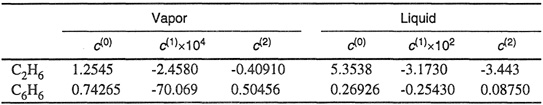
The experimental values (W. B. Kay and T. D. Nevens, 1952, Chem. Eng. Prog. Symp. Ser., 48: 108) are K_C2H6 = 2.73 and k_C6H6 = 0.41.

7. For the binary mixture of components 1 and 2, g^E at 0°C and 1 atm is expressed by g^EIRT = 1.877x₁x₂. For the same binary, the excess volumes were calculated as a function of pressure and composition; they are given by the equation (with pressure in atm),

v^E(cm³ mol^-1) = x₁x₂(4.026 - 0.233 In P) for 1 < P < 4000 atm.

This mixture is totally miscible at 0°C and 1 atm. At 0°C, find the lowest pressure at which phase separation will occur. When the same mixture is under 1500 atm pressure, what are the compositions of the two liquid phases in equilibrium?

8. For the equimolar mixture 2-propanol/n-heptane at normal pressure and 333 K, Van Ness et al. (1967, J. Chem. Eng. Data, 12: 217) report that h^E = 1445 J mol^-1. Using the volumetric data from Lichtenthaier et al. [Institute of Physical Chemistry, University of Heidelberg, Germany] quoted below, calculate h^E for the equimolar mixture at 333 K and 360 bar. For the equimolar mixture υ^E data are given in the form υ^E (cm³ mol^-1) = 0.25 A, where A depends on temperature and pressure:

9. Consider a binary gaseous mixture of carbon dioxide with a mole fraction of water equal to 0.2 at 150 atm. Find the temperature to which this mixture can be isobarically cooled without condensation. Assume that at this pressure the solubility of CO₂ in liquid water has a negligible effect.

In the calculations, use a modified form of the Redlich-Kwong equation of state where parameter a is given by a = a⁽⁰⁾ + a⁽¹⁾ where a⁽¹⁾ depends on temperature. USe a⁽⁰⁾(H₂O) = 35x10⁶ and a⁽⁰⁾(CO₂) = 46x10⁶ atm (cm³ mol^-1) K^1/2. Constants for finding a⁽¹⁾ are given in the table below. Use the normal mixing rules, but for the cross term a_ij include the equilibrium constant K (for the formation of a water-carbon dioxide complex) as follows: a_ij = [a_i⁽⁰⁾a_j⁽⁰⁾]^1/2 + 0.5R²T^2.5K. Constants for the temperature dependence of K (in atm^-1) are also given in the table. For water vapor, b = 14.6 cm³ mol^-1 and for carbon dioxide, b = 29.7 cm³ mol^-1. Data for pure saturated water can be obtained from the steam tables.

The temperature dependence of function X is given by

X = c₀ + c₁/T + c₂/T² + c₃/T³

where T is in kelvin.

10. For a solute in a supercritical solvent, the solubility minimum and maximum with pressure can be related to the partial molar volume of the solute in the fluid phase,

(a) Show that these solubility extrema can be predicted from

where subscript 2 refers to the solute; and are, respectively, the molar volume of the pure solid solute and the partial molar volume of the solute in the supercritical fluid phase; y₂ is the fluid-phase mole fraction; and φ₂ is the fluid-phase fugacity coefficient.

(b) As shown by Kurnik and Reid (1981, AIChE J., 27: 861), for naphthalene dissolved in ethylene, (∂ In φ2/∂ In y₂)_T,p is always more positive than -0.4 for all pressures to 4 kbar. Using the Redlich-Kwong equation of state and Eq. (12-41), calculate the pressures for solubility minimum and maximum at 318 K. Compare with experimental results.

For naphthalene at 318 K the vapor pressure and the solid density are 0.54 mmHg and 1.144 g cm^-3. Constants for Redlich-Kwong equation are: Ω_a = 0.4323, Ω_b = 0.0876 for ethylene, and Ω_a = 0.4497, Ω_b = 0.0915 for naphthalene. The binary parameter k₁₂ is equal to -0.0182. Molar volumes of ethylene at 318 K and as a function of pressure are shown in the following table: