Chapter 7
Fugacities in Liquid Mixtures:
Models and Theories of Solutions

When two or more pure liquids are mixed to form a liquid solution, it is the aim of solution theory to express the properties of the liquid mixture in terms of intermolecular forces and fundamental liquid structure. To minimize the amount of experimental information required to describe a solution, it is desirable to express the properties of a solution in terms that can be calculated completely from the properties of the pure components. Present theoretical knowledge has not yet reached a stage of development where this can be done with any degree of generality, although some results of limited utility have been obtained. Most current work in the theory of solutions utilizes the powerful methods of statistical mechanics that relate macroscopic (bulk) properties to microscopic (molecular) phenomena.¹

¹ For an introduction see, e.g., T. M. Reed and K. E. Gubbins, 1973, Applied Statistical Mechanics, (New York: McGraw-Hill); D. A. McQaarrie, 1985, Statistical Thermodynamics, (Mill Valley: University Science Books); T. L. Hill, 1986, An Introduction to Statistical Thermodynamics, (Reading: Addison-Wesley); and K. Lucas, 1991, Applied Statistical Thermodynamics, (Berlin: Springer). For more specialized discussions see T. Boublik, I. Nezbeda, and H. Hlavaty, 1980, Statistical Thermodynamics of Simple Liquids and Their Mixtures, (New York: Elsevier); K. Singer (Ed.), 1973, Statistical Mechanics, (London: The Royal Society of Chemistry); D. Chandler, 1987, Introduction to Modern Statistical Mechanics, (New York: Oxford University Press).

In this chapter, we introduce some of the theoretical concepts that have been used to describe and to interpret solution properties. We cannot give a complete treatment; we attempt, however, to give a brief survey of those ideas that bear promise for practical applications.

The simplest theory of liquid solutions is that due to Raoult, who set the partial pressure of any component equal to the product of its vapor pressure and its mole fraction in the liquid phase; at modest pressures, this simple relation often provides a reasonable approximation for those liquid solutions whose components are chemically similar. However, Raoult’s relation becomes exact only as the components of the mixture become identical, and its failure to represent the behavior of real solutions is due to differences in molecular size, shape, and intermolecular forces of the pure components. It appears logical, therefore, to use Raoult’s relation as a reference and to express observed behavior of real solutions as deviations from behavior calculated by Raoult’s law. This treatment of solution properties was formalized by Lewis in the early twentieth century, and since then it has become customary to express the behavior of real solutions in terms of activity coefficients. Another way of stating the aim of solution theory, then, is to say that it aims to predict numerical values of activity coefficients in terms of properties (or constants) that have molecular significance and that, hopefully, may be calculated primarily from the properties of the pure components.

One of the first systematic attempts to describe quantitatively the properties of fluid mixtures was made by van der Waals and his coworkers early in the twentieth century, shortly before the work of Lewis. Therefore, most of van der Waals’ work on fluid mixtures appears in a form that today strikes us as awkward. However, no one can deny that he and his colleagues at Amsterdam were the first great pioneers in a field that, since about 1890, has attracted the serious attention of a large number of outstanding physical scientists.² One of van der Waals’ students and later collaborators was van Laar, and it was primarily through van Laar’s work that the basic ideas of the Amsterdam school became well known. It is convenient, therefore, to begin by discussing van Laar’s theory of solutions and then to show how this simple but inadequate theory led to the more useful theory of regular solutions advanced by Scatchard and Hildebrand.

² Van der Waals’ thesis is translated by J. S. Rowlinson, 1988, Van der Waals: On the Continuity of the Gaseous and Liquid States, (Amsterdam: North-Holland). This book also contains insightful comments on the van der Waals theory of fluids from a modem point of view.

7.1 The Theory of van Laar

One of the essential requirements for a successful theory in physical science is judicious simplification. If one wishes to do justice to all the aspects of a problem, one very soon finds oneself in a hopelessly complicated situation. To make progress, it is necessary to ignore certain aspects of a physical situation and to retain others; the wise execution of this choice often makes the difference between a result that is realistic and one that is merely academic. Van Laar’s essential contribution was that he chose good simplifying assumptions that made the problem tractable and yet did not greatly violate physical reality.

Van Laar considered a mixture of two liquids: x₁ moles of liquid 1 and x₂ moles of liquid 2. He assumed that the two liquids mix at constant temperature and pressure in such a manner that:

1. There is no volume change, i.e., ν^E = 0.

2. The entropy of mixing is given by that corresponding to an ideal solution, i.e., S^E = 0,

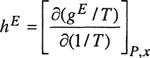
where superscript E stands for excess. Since, at constant pressure,

(7-1)

it follows from van Laar’s simplifying assumptions that

(7-2)

To calculate the energy change of mixing, van Laar constructed a three-step, isothermal, thermodynamic cycle wherein the pure liquids are first vaporized to some arbitrarily low pressure, mixed at this low pressure, and then recompressed to the original pressure, as illustrated in Fig. 7-1. The energy change is calculated for each step and, since energy is a state function independent of path, the energy change of mixing, Δu, is given by the sum of the three energy changes. That is,

(7-3)

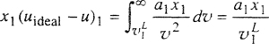
Step I. The two pure liquids are vaporized isothermally to the ideal-gas state. The energy change accompanying this process is calculated by the thermodynamic equation

(7-4)

Figure 7-1 Thermodynamic cycle for forming a liquid mixture from the pure liquids at constant temperature.

Van Laar then (unfortunately) assumed that the volumetric properties of the pure fluids are given by the van der Waals equation. In that case.

(7-5)

where α is the constant appearing in the van der Waals equation. With x₁ moles of liquid 1 and x₂ moles of liquid 2, we obtain exactly one mole of mixture. Then

(7-6)

and

(7-7)

where u_ideal energy of the ideal gas and ν^L is the molar volume of the pure liquid. Now, according to van der Waals’ theory, the molar volume of a liquid well below its critical temperature can be replaced approximately by the constant b. Thus

(7-8)

Step II. Isothermal mixing of gases at very low pressure (i.e.. ideal gases) proceeds with no change in energy. Thus

(7-9)

Step III. The ideal-gas mixture is now compressed isothermally and condensed at the original pressure. The thermodynamic equation (7-4) also holds for a mixture, and van Laar assumed that the volumetric properties of the mixture are also given by the van der Waals equation. Thus

(7-10)

It is now necessary to express constants a and b for the mixture in terms of the constants for the pure components. Van Laar used the expressions

(7-11)

(7-12)

Equation (7-11) follows from the assumption that only interactions between two molecules are important and that a_l2, the constant characteristic of the interaction between two dissimilar molecules, is given by the geometric-mean law. Equation (7-12) follows from the assumption that there is no volume change upon mixing the two liquids.

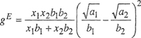
Equations (7-8) to (7-12) are now substituted in Eq. (7-3). Algebraic rearrangement gives

(7-13)

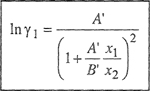
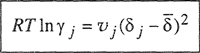
The activity coefficients are obtained by differentiation as discussed in Sec. 6.3 and we obtain

(7-14)

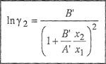
and

(7-15)

where

(7-16)

and

(7-17)

Equations (7-14) and (7-15) are the van Laar equations that relate the activity coefficients to temperature, composition, and to the properties of the pure components, i.e., (a₁, b₁) and (a₂, b₂).

Two important features of van Laar equations should be noted. One is that the logarithms of the activity coefficients are inversely proportional to the absolute temperature. This result, however, is independent of van Laar’s thermodynamic cycle and follows directly from the assumption that S^E = O.³ The other important feature is that according to van Laar’s theory, the activity coefficients of both components are never less than unity; hence, this theory always predicts positive deviations from Raoult’s law. This result follows from Eq. (7-11), which says that

³ At constant pressure and composition, the derivative of g^E with respect to temperature is -S^E. When S^E = 0, it follows that in γ is proportinai to T^-1 at constant pressure and composition.

(7-18)

whenever a₁ ≠ a₂.

Because constant α is proportional to the forces of attraction between molecules, Eq. (7-11) [or (7-18)] implies that the forces of attraction between the molecules in the mixture are less than what they would be if they were additive on a molar basis. If van Laar had assumed a rule where

(7-19)

he would have obtained

(7-20)

On the other hand, had he assumed that

(7-21)

he would have obtained that

(7-22)

Thus, we can see that the rules that one uses to express the constants for a mixture in terms of the constants for the pure components have a large influence on the predicted results.

As one might expect, quantitative agreement between van Laar’s equations and experimental results is not good. However, this poor agreement is not due as much to van Laar’s simplifications as it is to his adherence to the van der Waals equation and to the mixing rules used by van der Waals to extend that equation to mixtures.

One of the implications of van Laar’s theory is the relation between solution nonideality and the critical pressures of the pure components. According to van der Waals’ equation of state, the square root of the critical pressure of a pure fluid is proportional to . Therefore, van Laar’s theory predicts that the nonideality of a solution rises with increasing difference in the critical pressures of the components; for a solution whose components have identical critical pressures, van Laar’s theory predicts ideal behavior. These predictions, unfortunately, are contrary to experiment.

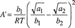
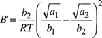
If we regard A′ and B′ as adjustable parameters, van Laar equations are useful empirical relations that have been used successfully to correlate experimental activity coefficients for many binary systems, including some that show large deviations from ideal behavior (see Sec. 6.10).

7.2 The Scatchard-Hildebrand Theory

Van Laar had recognized that a simple theory of solutions could be constructed if we restrict attention to those cases where the excess entropy and the excess volume of mixing could be neglected. Several years later, Hildebrand found that the experimental thermodynamic properties of iodine solutions in various nonpolar solvents appeared to be substantially in agreement with these simplifying assumptions. Hildebrand (1929) called these solutions regular and later defined a regular solution as one where the components mix with no excess entropy provided that there is no volume change upon mixing. Another way of saying this is to define a regular solution as one that has vanishing excess entropy of mixing at constant temperature and constant volume.

Both Hildebrand and Scatchard, working independently and a continent apart, realized that van Laar’s theory could be greatly improved if it could be freed from the limitations of van der Waals’ equation of state. This can be done by defining a parameter c according to

(7-23)

where Δ_vapu is the energy of complete vaporization, that is, the energy change upon isotherma! vaporization of the saturated liquid to the ideal-gas state (infinite volume). Parameter c is the cohesive-energy density.

Having defined c, the key step made by Hildebrand and Scatchard consisted in generalizing Eq. (7-23) to a binary liquid mixture by writing, per mole of mixture,

(7-24)

where superscript L has been dropped from the ν’s. Equation (7-24) assumes that the energy of a binary liquid mixture (relative to the ideal gas at the same temperature and composition) can be expressed as a quadratic function of the volume fraction and it also implies that the volume of a binary liquid mixture is given by the mole-fraction average of the pure-component volumes (i.e., V^E = 0). Constant c₁₁ refers to interactions between molecules of species 1; c₂₂ refers to interactions between molecules of species 2, and C₁₂ refers to interactions between unlike molecules. For saturated liquids, C₁₁ and c₂₂ are functions only of temperature.

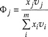
To simplify notation, we introduce symbols Φ₁ and Φ₂ that designate volume fractions of components 1 and 2, defined by

(7-25)

(7-26)

Equation (7-24) now becomes

(7-27)

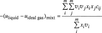
The molar energy change of mixing (that is also the excess energy of mixing) is defined by

(7-28)

Equation (7-23) (for each component) and Eq. (7-27) are now substituted into Eq. (7-28); also, we utilize the relation for ideal gases,

(7-29)

Algebraic rearrangement then gives

(7-30)

Scatchard and Hildebrand now make what is probably the most important assumption in their theory. They assume that for molecules whose forces of attraction are due primarily to dispersion forces, there is a simple relation between C₁₁, C₂₂ and C₁₂ as suggested by London’s formula (see Sec. 4.4), i.e.,

(7-31)

Substituting Eq. (7-31) into Eq. (7-30) gives

(7-32)

where

(7-33)

and

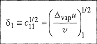
(7-34)

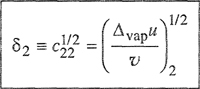
The positive square root of c is given the symbol δ, called the solubility parameter.

To complete their theory of solutions, Scatchard and Hildebrand make one additional assumption, i.e., that at constant temperature and pressure the excess entropy of mixing vanishes. This assumption is consistent with Hildebrand’s definition of regular solutions because in the treatment outlined above we had already assumed that there is no excess volume. With the elimination of excess entropy and excess volume at constant pressure, we have

(7-35)

The activity coefficients follow upon using Eq. (6-25). They are

(7-36)

and

(7-37)

Equations (7-36) and (7-37) are the regular-solution equations, and they have much in common with the van Laar relations [Eqs. (7-14) and (7-15)]. The regular-solution equations can easily be rearranged into the van Laar form by writing for parameters A′ and B′,

(7-38)

and

(7-39)

The regular-solution equations always predict γ_i ≥ 1; i.e., a regular solution can exhibit only positive deviations from Raoult’s law. This result is again a direct consequence of the geometric-mean assumption; it follows from Eq. (7-31), wherein the cohesive-energy density corresponding to the interaction between dissimilar molecules is given by the geometric mean of the cohesive-energy densities corresponding to interaction between similar molecules.

Solubility parameters δ₁ and δ₂ are functions of temperature, but the difference between these solubility parameters, δ₁ – δ₂, is often nearly independent of temperature. Since the regular-solution model assumes that the excess entropy is zero, it follows that at constant composition the logarithm of each activity coefficient must be inversely proportional to the absolute temperature. Hence, the model assumes that, as the temperature is varied at constant composition,

(7-40)

and

(7-41)

For many solutions of nonpolar liquids Eqs. (7-40) and (7-41) are reasonable approximations provided that the temperature range is not large and that the solution is remote from critical conditions.

Table 7-1 gives liquid molar volumes and solubility parameters for some typical nonpolar liquids at 25°C and for a few liquefied gases at 90 K. By inspection of the solubility parameters of different liquids, it is easily possible to make some qualitative statements about deviations from ideality of certain mixtures. Remembering that the logarithm of the activity coefficient varies directly as the square of the difference in solubility parameters, we can see, for instance, that a mixture of carbon disulfide with n-hexane exhibits large positive deviations from Raoult’s law, whereas a mixture of carbon tetrachloride and cyclohexane is nearly ideal. The difference in solubility parameters of mixture components provides a measure of solution nonideality. For example, the solubility parameters shown in Table 7-1 bear out the well-known observation that whereas mixtures of aliphatic hydrocarbons are nearly ideal, mixtures of aliphatic hydrocarbons with aromatics show appreciable nonideality.

Table 7-1 Molar liquid volumes and solubility parameters of some nonpoiar liquids.*

Regular-solution equations give a good semiquantitative representation of activity coefficients for many solutions containing nonpoiar components. Because of various simplifying assumptions that have been made in the derivation, we cannot expect complete quantitative agreement between calculated and experimental results, but for approximate work, i.e., for reasonable estimates of (nonpolar) equilibria in the absence of any mixture data, the regular-solution equations provide useful results.

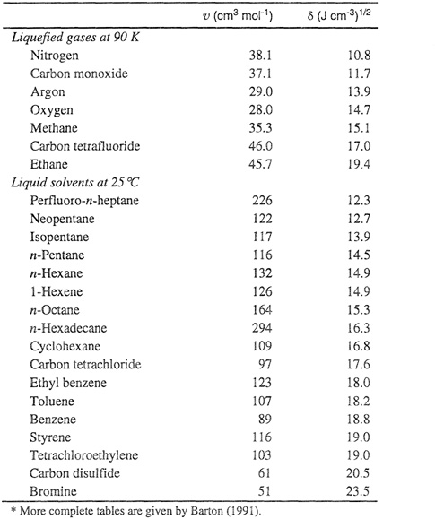
Figures 7-2, 7-3, and 7-4 show y-x diagrams for three representative nonpolar systems. Vapor-liquid equilibria were calculated first using Raoult’s law and then using the regular-solution equations; experimentally observed equilibria are also shown and it is evident that for two systems, results based on the regular-solution theory provide a considerable improvement over those calculated by Raoult’s law; for the third system, neopentane/carbon tetrachloride, the regular-solution equations overcorrect. For mixtures of nonpolar liquids, it is fair to say that whereas Raoult’s law gives a zeroth approximation, the regular-solution equations usually give a first approximation to vapor-liquid equilibria. While regular-solution results are not always good, for nonpolar systems they are usually reasonable, and whenever an estimate of phase equilibria is required, the theory of regular solutions provides a valuable guide. [It must again be emphasized that Eqs. (7-36) and (7-37) are not valid for solutions containing polar components]. The only major failure of the theory of regular solutions for nonpolar fluids appears to be when it is applied to certain solutions containing fluorocarbons (Scott, 1958); the reasons for this failure are only partly understood.

Figure 7-2 Vapor-liquid equilibria for CO (1)/CH₄(2) mixtures at 90.7 K.

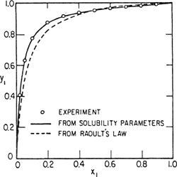
Figure 7-3 Vapor-liquid equilibria for C₆H₆ (1)/n-C₇H₁₆ (2) at70°C.

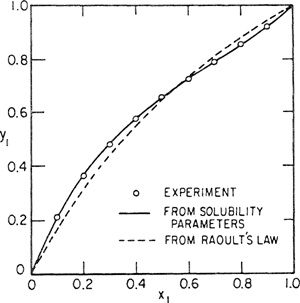
Figure 7-4 Vapor-liquid equilibria for neo-C₅H₁₂ (1)/CCl₄(2) at 0°C.

For mixtures that are nearly ideal, the regular-solution equations are often poor in the sense that predicted and observed excess Gibbs energies differ appreciably; however, for nearly ideal mixtures such errors necessarily have only a small effect on calculated vapor-liquid equilibria. For practical applications, the regular-solution equations are most useful for nonpolar mixtures having appreciable nonideality. Solubility-parameter theory provides a fairly good estimate of the excess Gibbs energies of most mixtures of common nonpolar liquids, especially when the excess Gibbs energy is large.

For small deviations from ideality, Eqs. (7-36) and (7-37) are less reliable because small errors in the geometric-mean assumption and in the solubility parameters become relatively more serious when δ₁ and δ₂ are close to one another.

Scott (1956) has shown that solubility-parameter theory fits excess Gibbs energies of most binary systems of nonpolar liquids to within 10 to 20% of the thermal energy RT. (At room temperature RT is nearly 2500 J mol^-1). McGlashan (1962) bears this out as indicated in Fig. 7-5, where a comparison is made between calculated and observed excess Gibbs energies for 21 binary systems near room temperature at the composition midpoint x₁ = x₂ = 1/2. The dashed lines were drawn 370 J mol^-1 (≈0.15RT) above and below the solid line that corresponds to perfect agreement between theory and experiment.

Figure 7-5 Excess Gibbs energies from the regular-solution equation. Binary systems shown are: 1. c-C₆H₁₂/CCl₄; 2. c-C₆H₁₂/C₆H₆; 3. c-C₆H₁₂/n-C₆H₁₄; 4. c-C₆H₁₂/C₆H₅CH₃; 5. c-C₆H₁₂/C(CH₃)₄; 6. C₆H₆/c-C₅H₁₀; 7. C₆CH₆/CCl₄; 8. C₆H₆/C₂H₄Cl₂; 9. CCl₄/CHCl₃; 10. CCl₄/C(CH₃)₄; 11. CCl₄/CH₃l; 12. TiCl₄/CCl₄; 13. SiCl₄/CCl₄; 14. C₆H₆/n-C₇H₁₆; 15.C₆H₆/n-C₆H₁₄; 16. C₆H₅CH₃/n-C₆H₁₄; 17. C₆H₅CH₃/n-C₇H₁₆; 18. C₆H₅CH₃/c-C₆H₁₁CH₃; 19. CCl₄/CH₂Cl₂; 20. n-C₆H₁₄/CCl₄; 21. C₆H₆/i-C₈H₁₈. Systems 8, 9, 11, and 19 each contain one component whose polarity is not negligible and, strictly speaking, they should not be included in this list. However, since there are no specific effects (e.g., hydrogen bonding) in these systems, regular-solution theory still gives the right order of magnitude for g^E for these particular mixtures. Most of the data are at 25°C. The lowest temperature (0°C) is for system 10 and the highest (65°C) for system 18. According to regular-solution theory, the excess Gibbs energy is independent of temperature to a first approximation. Dashed lines indicate ±0.15RT, here taken as ±370 J mol^-1.

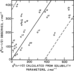
Figure 7-5 suggests that solubility parameters are primarily useful for semiquantitative estimates of activity coefficients in liquid mixtures. Solubility parameters can tell us readily the magnitude of nonideality that is to be expected in a mixture of two nonpolar liquids. In addition, solubility parameters can form a basis for a more quantitative application when modified empirically. One example of such an application is provided by Chao and Seader (1961), who used solubility parameters to correlate phase equilibria for hydrocarbon mixtures over a wide range of conditions. Two other applications, one concerned with gas solubility and the other with solubility of solid carbon dioxide at low temperatures, are discussed in later chapters.

The theory of Scatchard and Hildebrand is essentially the same as that of van Laar but it is liberated from the narrow confines of the van der Waals equation or of any other equation of state. We know that the assumptions of regularity (S^E = 0) and isometric mixing (ν^E = 0) at constant temperature and pressure are not correct even for simple mixtures but, due to cancellation of errors, these assumptions frequently do not seriously affect calculations of the excess Gibbs energy. (When regular-solution theory is used to calculate excess enthalpies, the results are usually much worse.) However, the most serious defect of the theory is the geometric-mean assumption. This assumption can be relaxed by writing instead of Eq. (7-31) the more general relation ⁴

⁴ The l₁₂ used here is related to, but different from, k₁₂ used in Sec. 5.7.

(7-42)

where l₁₂ is a constant, small compared to unity, characteristic of the 1-2 interaction. From London’s theory of dispersion forces, an expression can be obtained for l₁₂ in terms of molecular parameters but such an expression has little quantitative value.

In mixtures of chemically similar components (e.g., cyclohexane/n-hexane), deviations from the geometric mean are primarily a result of differences in molecular shape and subsequent differences in molecular packing. Our limited ability to describe properly the geometric arrangement of polyatomic molecules in the liquid phase is one of the main reasons for the inadequacy of currently existing theories of solution.

When Eq. (7-42) is used in place of Eq. (7-31), the activity coefficients are given by

(7-43)

and

(7-44)

Equations (7-43) and (7-44) show immediately that if δ₁ and δ₂ are close to each other, even a small value of l12 can significantly affect the activity coefficients. For example, suppose T = 300 K, ν₁ = 100 cm³ mol^-1, and δ₁ and δ₂ are 14.3 and 15.3 (J cm^-3)^1/2, respectively. Then, at infinite dilution, we find that for l12 = 0, = 1.04. However, if l12 = 0.03, we obtain = 1.77. Even if l12 is as small as 0.01, we obtain = 1.24. These illustrative results show why the solubility-parameter theory is not quantitatively reliable for components whose solubility parameters are very nearly the same. As the difference between δ₁ and δ₂ becomes larger, the effect of deviation from the geometric mean becomes less serious. However, it is apparent that even small deviations from the geometric mean, 1 or 2%, can have an appreciable effect on calculated activity coefficients and that much improvement in predicted results can often be achieved when only one (reliable) binary datum is available for evaluating l₁₂.

Efforts to correlate l₁₂ have met with little success. In his study of binary cryogenic mixtures, Bazúa (1971) found no satisfactory variation of l₁₂ with pure-component properties, although some rough trends were found by Cheung and Zander (1968) and by Preston (1970). In many typical cases l₁₂ is positive and becomes larger as the differences in molecular size and chemical nature of the components increase. For example, for carbon dioxide/paraffin mixtures at low temperatures, Preston found that l₁₂ = -0.02 (methane), +0.08 (ethane), +0.08 (propane), and +0.09 (butane).

Since l₁₂ is an essentially empirical parameter, it depends on temperature. However, for typical nonpolar mixtures over a modest range of temperature, that dependence is usually small.

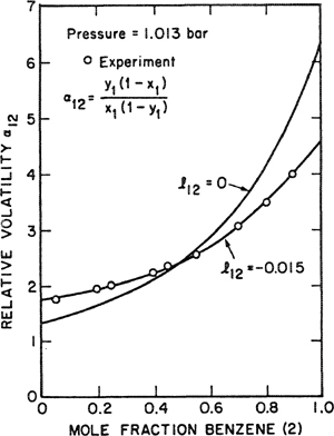
For mixtures of aromatic and saturated hydrocarbons, Funk (1970) found a systematic variation of l₁₂ with the structure of the saturated component, as shown in Fig. 7-6. In this case, a good correlation could be established because experimental data are relatively plentiful and because the correlation is restricted to a narrow class of mixtures. Figure 7-7 shows the effect of l₁₂ on calculating relative volatility in a typical binary system.

Figure 7-6 Binary parameter l₁₂ for aromatic-saturated hydrocarbon mixtures at 50°C. Binary systems shown are: 1. Benzene (2)/Pentane (1); 2. Benzene (2)/Neopentane (1); 3. Benzene (2)/Cyclopentane (1); 4. Benzene (2)/Hexane (1); 5. Benzene (2)/2-Methylpentane (1); 6. Benzene (2)/2,2-Dimethylbutane (1); 7. Benzene (2)/2,3-Dimethylbutane (1); 8. Benzene (2)/Cyclohexane (1); 9. Benzene (2)/Methylcyclopentane (1); 10. Benzene (2)/Heptane (1); 11. Benzene (2)/3-Methylhexane (1); 12. Benzene (2)/2,4-Dimethylpentane (1); 13. Benzene (2)/2,2,3-Trimethylbutane (1); 14. Benzene (2)/Methylcyclohexane (1); 15. Benzene (2)/Octane (1); 16. Benzene (2)/2,2,4-Trimethylpentane (1); 17. Toluene (2)/Hexane (1); 18. Toluene (2)/3-Methylpentane (1); 19. Toluene (2)/Cyclohexane (1); 20. Toluene (2)/Methylcyclopentane (1); 21. Toluene (2)/Heptane (1); 22. Toluene (2}/Methylcyclohexane (1); 23. Toluene (2)/2,2,2,4-Trimethylpentane (1).

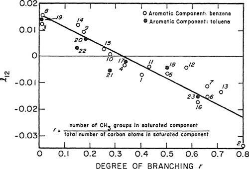
Figure 7-7 Comparison of experimental volatilities with volatilities calculated by Scatchard-Hildebrand theory for 2,2-dimethylbutane (1)/benzene (2).

Our inability to correlate l₁₂ for a wide variety of mixtures follows from our lack of understanding of intermolecular forces, especially between molecules at short separations.

One of the early improvements in the regular-solution theory was to replace the ideal entropy of mixing with the Flory-Huggins equations for mixing molecules appreciably different in size (Sec. 8.2). Another improvement was proposed by Gonsalves and Leland (1978) using some theoretical knowledge about the structure (molecular packing) of a fluid mixture. The results for their modified regular-solution theory show an improvement in the calculated excess Gibbs energy and excess enthalpy when the molecules in the mixture differ appreciably in size and shape. For molecules of approximately the same size, the modified theory gives essentially the same results as those from the original regular-solution theory.

The most important assumption in the calculation of excess functions is the one that concerns the unlike-pair interaction. Small errors in predicting this interaction can often offset completely any improvement derived from a better description of liquid structure.

Several authors have tried to extend regular-solution theory to mixtures containing polar components, but unless the classes of components considered are restricted, such extension has only semiquantitative significance. In establishing these extensions, the cohesive energy density is divided into separate contributions from nonpolar (dispersion) forces and from polar forces:

(7-45)

Equations (7-43) and (7-44) are used with the substitutions

(7-46)

(7-47)

(7-48)

where λ_i is the nonpolar solubility parameter and τ_i is the polar solubility parameter . Binary parameter ψ₁₂ is not negligible, as shown by Weimer (1965) in his correlation of activity coefficients at infinite dilution for hydrocarbons in polar non-hydrogen-bonding solvents.

Further extension of the Scatchard-Hildebrand equation to include hydrogen-bonded components makes little sense theoretically, because the assumptions of regular-solution theory are seriously in error for mixtures containing such components. Nevertheless, some semiquantitative success has been achieved by Hansen et al. (1967, 1967a, 1971) and others (Burrell, 1968; Gardon, 1966; Nelson et al., 1970; Mark et al., 1969; Barton, 1991) interested in establishing criteria for formulating solvents for paints and other surface coatings. Also, Null and Palmer (1969) and Null (1970) have used extended solubility parameters for establishing an empirical correlation of activity coefficients. Barton (1991) has given a comprehensive review of extended solubility parameters and their applications. Panayiotou (1997) has developed an equation of state model that provides analytical expressions to estimate solubility parameters as functions of temperature, pressure and mixture composition. This model is general, also applicable to complex systems containing molecules forming hydrogen bonds.

One of the main advantages of the regular-solution equations is their simplicity, and this simplicity is retained when the regular-solution model is extended to solutions containing more than two components. The derivation for the multicomponent case is analogous to that given for the binary case. The molar energy of a liquid mixture containing m components is written

(7-49)

The volume fraction of component j is now defined by

(7-50)

and the excess energy of mixing is defined by

(7-51)

By assumption, the cohesive-energy density c_ij is given by the geometric mean,

(7-52)

Again assuming that

(7-53)

we again have

(7-54)

Substitution and algebraic rearrangement, coupled with Eq. (6-25), gives a remarkably simple result for the activity coefficient of component j in a multicomponent solution:

(7-55)

where

(7-56)

Parameter is a volume-fraction average of the solubility parameters of all the components in the solution; the summation in Eq. (7-56) is over all components, including component j.

Equation (7-55) has the same advantages and disadvantages as Eqs. (7-36) and (7-37). It is useful for providing estimates of equilibria in nonpolar solutions and, with empirical modifications, it can serve as a basis for quantitative correlations.

Equations (7-43) and (7-44) can also be generalized for mixtures containing more than two components; the general expression for the activity coefficient, however, is no longer as simple as that given by Eq. (7-55). For a mixture of m components, it is

(7-57)

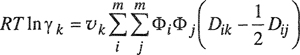
where

(7-58)

For every component i, l_ii=D_ii = 0. Equation (7-57) reduces to Eq. (7-55) only if l_ij=0 for every ij pair.

Regular-solution theory is attractive because of its simplicity. For many liquid mixtures that contain nonpolar molecules, this theory can predict equilibria with fair accuracy and for many more, it can correlate liquid-phase activity coefficients using only one adjustable parameter to correct for deviations from the geometric-mean as sumption.

For mixtures that contain large molecules (polymers) or for those that contain strongly polar or hydrogen-bonding molecules, the theory of regular solutions is in adequate; for such mixtures other theories are better, as described later in this chapter and in Chap. 8. However, before turning to such mixtures, it is useful to discuss briefly an alternate procedure applicable, in principle, to all fluid mixtures, although in practice it is usually applied only to relatively simple mixtures. This procedure is based on an equation of state applied to both the vapor phase and the liquid phase, following equations given in Sec. 3.4. This procedure is also discussed in Chapter 12.

7.3 Excess Functions from an Equation of State

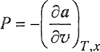
For a liquid mixture, we can calculate the conventional molar excess Gibbs energy g^E provided that we have available an equation of state that is valid for the entire density range from zero to liquid density.

Because a realistic equation of state is inevitably pressure-explicit, it is more convenient to calculate the molar excess Helmholtz energy a^E. As shown elsewhere,⁵ at low pressures, we can use the excellent approximation

⁵ J. H. Hildebrand, J. M. Prausnitz, and R. L. Scott, 1970, Regular and Related Solutions, New York: Van Nostrand Reinhoid.

(7-59)

where subscript v indicates constant volume and subscript P indicates constant pressure. The relation between molar Helmholtz energy, a, and the equation of state is discussed in Chap. 3; the fundamental working equation is

(7-60)⁶

⁶ To avoid conftision with equation-of-sfaie parameter a, we use In this section a for molar Helmholtz energy.

where subscript x indicates constant composition and is the molar volume. To illustrate, we use the Frisch-van der Waals equation of state,

(7-61)

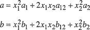
where reduced density and where, for a binary mixture, constants a and b are given by customary mixing rules quadratic in mole fraction x:

(7-62)

For binary parameter b₁₂ we write

(7-63)

and for the other binary parameter,

(7-64)

where, for simple mixtures,

Equation (3-50) is used to find Helmholtz energy A for the mixture, for pure liquid 1 and for pure liquid 2. The molar excess Helmholtz energy a^E is given by

(7-65)

where a=A/n_T, n_T is the total number of moles, and v^*_mixt=x₁v₁+x₂v₂. Here v₁ is the molar volume of pure liquid 1 and v₂ is the molar volume of pure liquid 2, it being understood that system temperature T is well below T_c1 and T_C2, where T_c is the critical temperature. Upon substituting Eq. (3-50) into Eq. (7-65), constants u_i⁰ and s_i⁰ cancel out.

Using a_v^E=g_p^E, we can find the molar excess enthalpy h^E by differentiating

(7-66)

where it is understood that both g^E and h^E refer to mixing at constant temperature and pressure.

The molar excess volume ^E is found by solving the equation of state three times, once for the mixture, once for pure liquid 1, and once for pure liquid 2:

(7-67)

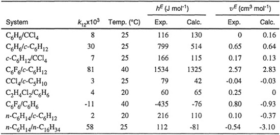
Calculations to obtain excess functions have been performed by Marsh (1980) for nine binary systems. For each pure liquid, constants a and b were found from critical data. Binary parameter k₁₂ was found from the experimental g^E at x₁=x₂=0.5.

Table 7-2 shows experimental and predicted h^E and V^E for equimolar mixtures. Agreement is fair for mixtures of nearly spherical molecules (first six systems) but it is poor for C₆F₆/C₆H₆, where there is an enhanced interaction between unlike molecules (negative k₁₂), and for the last two systems where the molecules no longer have even approximately spherical shape.

Table 7-2 Experimental and predicted molar excess enthalpies and molar excess volumes for nine equimoiar liquid mixtures (Marsh, 1980).

Some promising efforts have been made to construct equations of state for non-spherical molecules and it is likely that these will become increasingly useful for liquid mixtures containing such molecules, as discussed later in this chapter and in Chap. 8. However, for practical calculations, it is often convenient to abandon the equation-of-state approach and to use, instead, approximate theories of solutions based on the idea that in the condensed state, molecules arrange themselves in a lattice-like structure where each molecule (or molecular segment) occupies one lattice point. These ideas are discussed in the next sections.

7.4 The Lattice Model

Since the liquid state is in some sense intermediate between the crystalline state and the gaseous state, it follows that there are two types of approach to a theory of liquids. The first considers liquids to be gas-like; a liquid is pictured as a dense and highly nonideal gas whose properties can be described by some equation of state; that of van der Waals’ is the best known example. An equation-of-state description of pure liquids can readily be extended to liquid mixtures as was done by van der Waals and by some of his disciples like van Laar and later by many others.

The second approach considers a liquid to be solid-like, in a quasicrystalline state, where the molecules do not translate fully in a chaotic manner as in a gas, but where each molecule tends to stay in a small region, a more or less fixed position in space about which it vibrates back and forth. The quasicrystalline picture of the liquid state supposes molecules to sit in a regular array in space, called a lattice, and therefore liquid and liquid mixture models based on this simplified picture are called lattice models.⁷. These theories are described in detail elsewhere (Barker, 1963; Guggenheim, 1966) and their proper study requires familiarity with the methods of statistical mechanics. We give here only a brief introduction to the lattice theory of solutions.

⁷ An exhaustive attempt has been made by Eyring and coworkers to describe liquids as consisting of gas-Sike and solid-like molecules (H. Eyring and M. S. John, 1969, Significant Liquid Structures, New York: John Wiley & Sons). While this attempt has had some empirical success, its main ideas and assumptions are in direct conflict with many physicoehemical data for liquid structure.

Since the lattice theory of liquids assumes that molecules are confined to lattice positions (sometimes called cages), calculated entropies (disorder) are low by what is called the “communal entropy”. While this is a serious deficiency, it tends to cancel when lattice theory is used to calculate excess properties of liquid mixtures.

Molecular considerations suggest that deviations from ideal behavior in liquid solutions are due primarily to the following effects: First, forces of attraction between unlike molecules are quantitatively different from those between like molecules, giving rise to a nonvanishing enthalpy of mixing; second, if the unlike molecules differ significantly in size or shape, the molecular arrangement in the mixture may be appreciably different from that for the pure liquids, giving rise to a nonideal entropy of mixing; and finally, in a binary mixture, if the forces of attraction between one of three possible pair interactions are very much stronger (or very much weaker) than those of the other two, there are certain preferred orientations of the molecules in the mixture that, in extreme cases, may induce thermodynamic instability and demixing (incomplete miscibility).

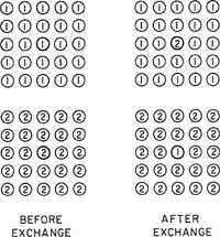
We consider a mixture of two simple liquids 1 and 2. Molecules of types 1 and 2 are small and spherically symmetric and the ratio of their sizes is close to unity. We suppose that the arrangement of the molecules in each pure liquid is that of a regular array as indicated in Fig. 7-8; all the molecules are situated on lattice points that are equidistant from one another. Molecular motion is limited to vibrations about the equilibrium positions and is not affected by the mixing process. We suppose further that for a fixed temperature, the lattice spacings for the two pure liquids and for the mixture are the same, independent of composition (i.e., ^E= 0).

Figure 7-8 Physical significance of interchange energy. The energy absorbed in the process above is 2w. [See Eq. (7-71)].

To derive an expression for the potential energy of a liquid, pure or mixed, we assume that the potential energy is pairwise additive for all molecular pairs and that only nearest neighbors need be considered in the summation. This means that the potential energy of a large number of molecules sitting on a lattice is given by the sum of the potential energies of all pairs of molecules that are situated immediately next to one another. For uncharged nonpolar molecules, intermolecular forces are short-range and therefore we assume in this simplified discussion that we can neglect contributions to the total potential energy from pairs that are not nearest neighbors.

Consider that each of N₁ molecules of type 1 and N₂ molecules of type 2 has z nearest (touching) neighbors, (z is the coordination number and may have a value between 6 and 12 depending on the type of packing, i.e., the way in which the molecules are arranged in three-dimensional space; empirically, for typical liquids at ordinary conditions, z is close to 10.) The total number of nearest neighbors is (z/2)(N₁+ N₂) and there are three types of nearest neighbors: 1-1, 2-2, and 1-2. Let N₁₁ be the number of nearest-neighbor pairs of type 11, N₂₂ that of type 22, and N₁₂ that of type 12. These three numbers are not independent; they are restricted by the following conservation equations:

(7-68)

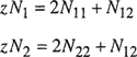
The total potential energy of the lattice U_t is then given by

(7-69)

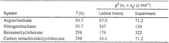
where, as in Chap. 4, Γ₁₁ is the potential energy of a 1-1 pair, Γ₂₂ that of a 2-2 pair, and Γ₁₂ that of a 1-2 pair. Substitution of N₁₁ and N_>22 from Eq. (7-68) gives

(7-70)

where w, the interchange energy, is defined by

(7-71)

Equation (7-70) gives the potential energy of a binary mixture and also that of a pure liquid; in the latter case, N₁₂ and either N₁ or N₂ are set equal to zero. In Eq. (7-70), the last term is the energy of mixing.

The physical significance of w is illustrated in Fig. 7-8; z pairs of type 1 and z pairs of type 2 are separated to form 2z dissimilar (1-2) pairs. Therefore, the change in energy that accompanies the interchange process shown in Fig. 7-8 is equal to 2w.

To obtain thermodynamic properties, it is convenient to calculate first the canonical partition function (see App. B) of the lattice, given by

(7-72)

where g is the combinatorial factor (degeneracy).⁸ equal to the number of ways of arranging N₁ molecules of type 1 and N₂ molecules of type 2 on a lattice with a total of (N₁+ N₂) sites. For a pure component, whose molecules are of the type discussed here, g = 1. The summation over all N₁₂ that give the same U_t can be replaced by retaining only the maximum term (see App. B).

⁸ Combinational factor g should not be confused with molar Gibbs energy g.

For the Helmholtz energy change of mixing we have

(7-73)

Using the relation between Helmholtz energy and the canonical partition function given in App. B (Table B-1), we obtain

(7-74)

Our task now is to say something about N ₁₂. In view of the similarity between the two types of molecules, we assume that a mixture of 1 and 2 is completely random, i.e., a mixture where ail possible arrangements of the molecules on the lattice are equally probable. For that case let N₁₂ =N^*₁₂. By simple statistical arguments it can be shown (Guggenheim, 1952) that for a completely random arrangement,

(7-75)

and

(7-76)

Substitution of Eqs. (7-75) and (7-76) into Eq. (7-74) and Stirling’s approximation⁹ gives

⁹ In N1=N 1n N-N, when N is large (see App.B.).

(7-77)

or, in molar units,

(7-78)

Notice that Eq, (7-78) is symmetric with respect to mole fraction x. For w = 0 we obtain an ideal solution; therefore, the molar excess Helmholtz energy is

(7-79)

Since w is independent of temperature (by assumption), we obtain for the entropy of mixing

(7-80)

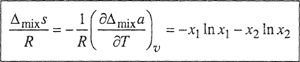
This is the entropy of mixing for an ideal solution (w = 0); for this type of mixture, the excess entropy is zero (S^E= 0).

In view of the assumptions made about the lattice spacing for pure liquids and the mixture, we assume that the mixing process at constant pressure and temperature prodaces no changes in volume (^E= 0).

As indicated in Sees. 7.1 and 7.2 (theories of van Laar and of Scatchard and Hil debrand), a solution for which s^E= ^E= 0 is called a regular solution.

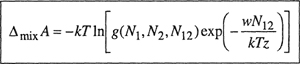
For a regular solution the excess Gibbs energy, the excess Helmholtz energy, the excess enthalpy (or enthalpy of mixing) and the excess energy (or energy of mixing) are all equal:

(7-81)

where N_A is Avogadro’s constant. The activity coefficients follow from Eq. (6-25):

(7-82)

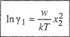
(7-83)

These results are of the same form as that of the two-suffix Margules equations. However, in Eqs. (7-82) and (7-83) parameter w has a well-defined physical significance.

From Eq. (7-71) we see that if the potential energy for a 1-2 pair is equal to the arithmetic mean of the potentials for the 1-1 and 2-2 pairs, then w = 0 and γ₁= γ₂=1 for all x; we then have an ideal solution. However, as discussed in Chap. 4, for simple, nonpolar molecules Γ₁₂ is more nearly equal to the geometric mean than to the arithmetic mean of Γ₁₁ and Γ₂₂. Because the magnitude of the geometric mean is always less than that of the arithmetic mean, and since Γ_i2, Γ₁₁, and Γ₂₂ are negative in sign, it follows that for mixtures of simple, nonpolar molecules, Eqs. (7-82) and (7-83) predict positive deviations from ideal-solution behavior, in agreement with experiment.

7.5 Calculation of the Interchange Energy from Molecular Properties

Because the interchange energy w is related to the potential energies, it should be possible to obtain a numerical value for w from information on potential functions. Various attempts to do this have been reported and one of them, doe to Kohler (1957), is particularly simple.

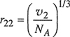
The potential function Γ depends on r, the distance between molecules. Kohler assumes that for the pure liquids,¹⁰

¹⁰ These assumptions are not completely consistent with the assumptions of the lattice theory, where r₁₁ = r₂₂= r₁₂. Strictly, the lattice theory requires that ₁ = ₂, and that very much limits its applicability. A certain degree of inconsistency frequently results when an idealized theory is applied to real phenomena.

(7-84)

and

(7-85)

where v stands for the molar liquid volume and N_A is Avogadro’s constant. In the mixture, Kohler assumes

(7-86)

Basing his calculations on London’s theory of dispersion forces (see Chap. 4), Kohler then writes ¹¹

¹¹ ξ is closely related to the ionization potential (see Sec. 4.4).

(7-87)

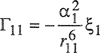
(7-88)

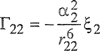
(7-89)

where α is the polarizability and ξ_i is calculated from Δ_vaph_i, the molar enthalpy of vaporization, by

(7-90)

When these expressions are substituted into Eq. (7-71), it is possible to obtain the interchange energy w as needed in the calculation of activity coefficients, Eqs. (7-82) and (7-83). One of the advantages of Kohler’s method is that, because of cancellation, no separate estimate of the coordination number z is required; further, the three potential energies Γ₁₁, Γ₂₂, and Γ₁₂ are calculated separately and it is not necessary to assume that Γ₁₂ is the geometric mean of the other two.

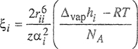
Using Kohler’s method, calculations have been made for the excess Gibbs energies of four simple binary systems, each at the composition midpoint where x_l= x₂ =0.5. Calculated results are compared in Table 7-3 with experiment and agreement is fairly good. However, we must remember that the applicability of this type of calculation is limited to mixtures where the molecules of the two components are not only nonpolar but also essentially spherical and similar in size. As a result, the equations that we have described are useful only for a small class of mixtures; when calculations based on Kohler’s method are made for systems outside of this small class, agreement with experiment is usually poor.

Table 7-3 Excess Gibbs energies for equimolar, binary mixtures. Calculations based on lattice theory and Kohler’s method for evaluating the interchange energy.

Numerous efforts have been made to extend calculations similar to those of Kohler to more complex systems. In genera!, they are not successful because of our inadequate understanding of intermolecular forces. With few exceptions, we cannot predict forces between dissimilar species, using only experimental data for similar species. At present, a reasonable procedure for testing a theory is to fit that theory to one binary experimental property and then to see if that theory can predict other binary properties. This was the procedure used by Marsh, shown in Table 7-2.

7.6 Nonrandom Mixtures of Simple Molecules

One of the important assumptions made in the previous sections was that when the molecules of two components are mixed, the arrangement of the molecules is completely random; i.e., the molecules have no tendency to segregate either with their own kind or with the other kind of molecule. In a completely random mixture, a given molecule shows no preference in the choice of its neighbors.

Because intermolecular forces operate between molecules, a completely random mixture in a two-component system of equisized molecules can only result if these forces are the same for all three possible molecular pairs 1-1, 2-2, and 1-2.’¹² In that event, however, there would also be no energy change upon mixing. Strictly, then, only an ideal mixture can be completely random.

¹² The model based on the lattice theory is not so restrictive. For molecules of the same size, there is no energy of mixing and no departure from randomness when the interchange energy is zero, i.e., when Γ₁₂ = 1/2(Γ₁₁+ Γ₂₂).

In a mixture where the pair energies F₁₁,F₂₂, and F₁₂ are not the same, some ordering (nonrandomness) must result. For example, suppose that the magnitude of the attractive energy between a 1-2 pair is much larger than that between a 1-1 and 2-2 pair; in that case, there is a strong tendency to form as many 1-2 pairs as possible. An example of such a situation is provided by the system chloroform/acetone, where hydrogen bonds can form between unlike molecules but not between like molecules. Or, suppose that the attractive forces between a 1-1 pair are much larger than those between a 1-2 or a 2-2 pair; in that event, a molecule of type 1 prefers to surround itself with other molecules of type 1 and more 1-1 pairs exists in the mixture than would exist in a purely random mixture having the same composition. An example of such a situation is the diethyl ether/pentane system; because diethyl ether has a large dipole moment whereas pentane is nonpolar, ether molecules interact by dipole-dipole forces that, on the average, are attractive; but between ether and pentane and between pentane and pentane there are no dipole-dipole forces.

In the lattice theory (for w independent of T), entropy is a measure of randomness; the entropy of mixing for a completely random mixture [Eq. (7-80)] is always larger than that of a mixture that is incompletely random, regardless of whether non-randomness is due to preferential formation of 1-2 or 1-1 (or 2-2) pairs. Excess entropy due to ordering (i.e., nonrandomness) is always negative.

Guggenheim (1952) has constructed a lattice theory for molecules of equal size that form mixtures that are not necessarily random. This theory is not rigorous but utilizes a simplification known as the quasichemical approximation. The essential ideas of this theory are summarized below.

For a completely random mixture, we set N₁₂ = N^*₁₂, given by Eq. (7-75), where * designates complete randomness. If w < 0, we expect N₁₂ > N^*₁₂ (e.g. chloroform/acetone), and if w > 0, we expect N₁₂>N^*₁₂ (e.g. diethyl ether/pentane). Now consider the “reaction”

(7-91)

For this “reaction” a chemical equilibrium constant K is defined by

(7-92)

According to Eq. (7-71), the energy change for this “reaction” is 2w/z. From thermodynamics, the temperature derivative of In K is

(7-93)

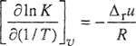
where Δ_rμ is the molar energy change of the “reaction”. We assume that Δ_rμ is independent of temperature and that

(7-94)

Integration gives

(7-95)

where C is a constant, independent of w and T. We can find C from the limiting case w = 0, i.e., when mixing is completely random:

(7-96)

where * designates random mixing. Using N^*₁₂ given by Eq. (7-75) and the two conservation Eqs. (7-68), we obtain from Eq. (7-96) C = 4.

Combination of Eqs. (7-92) and (7-95) gives the key relation between N₁₂, N₁₁, and N₂₂:

(7-97)

where η = exp(w/zkT).

We now relate N₁₂ to N^*₁₂ by introducing a parameter β according to

(7-98)

For the random case, β = 1. Using Eq. (7-97) and the conservation equations, Eq. (7-68), we find that β is given by

(7-99)

where x is the mole fraction. When w = 0 (η² 1),β = 1, as expected. As used here, β depends not only on w, but also on the composition (x₁, x₂). For w > 0, we obtain η² > 1 and β > 1 and therefore, N₁₂ <N^*₁₂ for w < 0, we obtain η² < 1 and β < 1; therefore, N₁₂ >N^*₁₂ As wlkT → ∞ η² β → ∞ and β → ∞ therefore, N₁₂ → 0 (no mixing at all). As wlkT -→ ∞, η²→ 0, and β → 0 (at X₁ = x₂= 0.5) and, therefore, N₁₂→2N^*₁₂ This case corresponds to formation of a stable 1-2 complex.

From Eqs. (7-98) and (7-70), the excess energy of mixing is

(7-100)

where u^E* is the excess energy for the completely random mixture given by Eq. (7-81). The excess Helmholtz energy is obtained by integrating the thermodynamic equation

(7-101)

The boundary condition is β → 1 as T →∞ (complete randomness). The integration again assumes that w is independent of temperature. However, as indicated by Eq. (7-99), τ is temperature dependent. The result for the molar excess Helmholtz energy is

(7-102)

If β = 1, a^E = 0, as expected. However, β = 1 only when wlkT = 0, corresponding to an ideal solution. Equation (7-102) shows that a^E depends on z, whereas in the simpler approximation [Eq. (7-79)], a^E is independent of z.

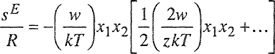
Equation (7-102) can be simplified if we restrict attention to moderate values of wlzkT). For most cases, w/zkT is smaller than unity and therefore we can expand the exponential ep(2w/zkT) that appears in Eqs. (7-99) and (7-102). Neglecting higher terms, the molar excess functions are

(7-103)

(7-104)

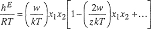
(7-105)

All excess functions are symmetric in x. However, excess Gibbs energy is no longer equal to excess enthalpy and excess entropy is no longer zero. Only in the limit, as (2w/zkT) → 0, we obtain

as expected. In other words, the earlier results based on the assumption of complete randomness become a satisfactory approximation as the interchange energy per pair of molecules becomes small relative to the thermal energy kT. For a given mixture, randomness increases as the temperature rises or, at a fixed temperature, randomness increases as the interchange energy falls.

The excess entropy given by Eq. (7-105) is never positive; for any nonvanishing value of w, positive or negative, S^E is always negative. For this particular model, therefore, the entropy of mixing is a maximum for the completely random mixture.¹³ However, the contribution of nonrandomness to the excess Gibbs energy and to the excess enthalpy may be positive or negative, depending on the sign of the interchange energy.

¹³ For many nonpolar mixtures of nearly equi-sized molecules, positive excess entropies have been observed experimentally. These observations are a result of other effects (neglected by the lattice theory) such as changes in volume and changes in excitation of internal degrees of freedom (rotation, vibration) that may result from the mixing process.

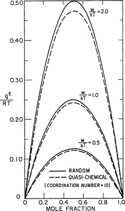
The excess Gibbs energy, given by Eq. (7-103) based on the quasichemical approximation, is not very different from Eq. (7-81) based on the assumption of random mixing. Figure 7-9 compares excess Gibbs energies calculated by the two equations and it is evident that for totally miscible mixtures the correction for nonrandom mixing is not large.

Figure 7-9 Effect of nonrandomness on excess Gibbs energies of binary mixtures.

However, deviations from random mixing become significant when wlkT is large enough to induce limited miscibility of the two components. The criteria for incipient demixing (instability) are¹⁴

¹⁴ see Sec. 6.12.

(7-106)

where Δ_mixg is the change in the total (not excess) molar Gibbs energy upon mixing:

(7-107)

When Eq. (7-81) is substituted into Eq. (7-106), we find that T^c, the upper consolute temperature, is given by

(7-108)

The upper consolute temperature is the maximum temperature for limited miscibility: for T > T^c there is only one stable liquid phase (complete miscibility), whereas for T <T^c there are two stable liquid phases.

In contrast to Eq. (7-108), when results based on the quasichemical approximation are substituted into Eq. (7-106), we obtain

(7-109)

When z = 10, we find

(7-110)

Equation (7-110) shows that the consolute temperature according to the quasi-chemical approximation, is about 10% lower than that computed from the assumption of random mixing. This is a significant change, although when compared to experiment, it is not sufficiently large. However, a large effect becomes noticeable when we compute the coexistence curve, the locus of mutual solubilities of the two components at temperatures below the upper consolute temperature.

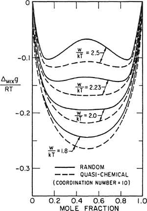
Figure 7-10 shows calculated results for the change in Gibbs energy due to mixing for four values of w/kT; calculations were performed first, assuming random mixing and second, assuming the quasichemical approximation. When wlkT = 1.8, both theories predict complete miscibility. When w/kT= 2.0, the random-mixing theory predicts incipient instability, whereas the quasichemical theory predicts complete miscibility. When w/kT = 2.23, the random theory indicates the existence of two liquid phases whose compositions are given by the two minima in the curves; the more refined theory merely predicts incipient dernixing. When w/kT - 2.5, both theories indicate the existence of two liquid phases, but the compositions of the two phases as given by one theory are different from those given by the other. These compositions are given by the minima in the curves and we see that the mutual solubilities predicted by the quasichemical approximation are about twice those predicted by the random-mixing assumption. These illustrative calculations show that the effect of ordering (i.e., nonrandomness) is not important except when the components are near or below their consolute temperature.

Figure 7-10 Effect of nonrandomness on Gibbs energy of mixing.

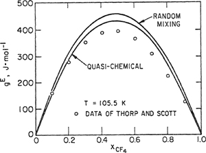
As a further illustration, we show in Figs. 7-11 and 7-12 some calculations of Eckert (1964) for the methane/carbon tetrafluoride system. From second-virial-coefficieet data for mixtures of the two gases near room temperature, Eckert estimates the interchange energy [Eq. (7-71)] and then calculates the excess Gibbs energy at 105.5 K for the liquid mixture. The results are shown in Fig. 7-11 along with the experimental data of Thorp and Scott (1956); agreement with experiment is good and there is not much difference between calculations based on random mixing and those based on the quasi-chemical approximation.

Figure 7-11 Excess Gibbs energy of methane/carbon tetrafluoride system.

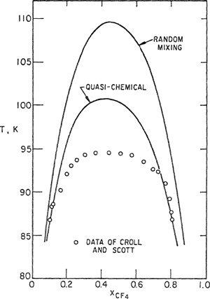
Croll and Scott (1958) have observed that methane and carbon tetrafluoride are not completely miscible below about 94 K; Eckert therefore calculated the coexistence curve and the results are shown in Fig. 7-12. The random-mixing theory predicts a consolute temperature that is too high by about 15 K; the consolute temperature predicted by the quasichemical theory is also too high but considerably less so. It is clear from Fig. 7-12 that for calculation of mutual solubilities in a pair of incompletely miscible liquids, the quasichemical theory provides a significant improvement over the random mixing theory. However, even in the improved theory there are still many features that are known to be incorrect. While the quasichemical theory is a step in the right direction, it provides no more than an approximation that is still far from a satisfactory theory of liquid mixtures.

Figure 7-12 Liquid-liquid coexistence curve for the methane/carbon telrafluoride system.

7.7 The Two-Liquid Theory

Extension of a corresponding-states theory to mixtures is based on the fundamental idea that a mixture can be considered to be a hypothetical pure fluid whose characteristic molecular size and potential energy are composition averages of the characteristic sizes and energies of the mixture’s components (one-fluid theory). In macroscopic terms, effective critical properties (pseudocriticals) are composition averages of the component critical properties. However, this fundamental idea is not limited to one hypothetical pure fluid; it can be extended to include more than one hypothetical fluid, leading to m-fluid theories. These theories use as a reference a suitable (usually mole-fraction) average of the properties of m hypothetical pure fluids (Hicks, 1976). For example, two-fluid theories, as discussed by Scott (1956) and by Leland et al. (1969), use two pure reference fluids. For simple mixtures, one-fluid and two-fluid theories give similar results when compared with experiment (Henderson and Leonard, 1971). Watson and Rowlinson (1969), for example, have obtained good agreement between experimental and calculated bubble points for the ternary system argon/nitrogen/oxygen and the three corresponding binary systems.¹⁵ Table 7-4 shows results for the nitrogen/oxygen system. In the entire pressure range, the differences between one-fluid and two-fluid models are small.

Table 7-4 Calculation of bubble temperatures of the system nitrogen/oxygen.

¹⁵ Vera and Prausnitz (1971, Chem. Eng. Sci., 26: 1772), have presented similar calculations for these systems using a reduced equation of state.

Because one-fluid theory is easier to use, it is usually preferred. However, two-fluid theory provides a useful point of departure for deriving semiempirical equations to represent theraiodynamic excess functions for highly nonideal mixtures. To illustrate, we present first a brief discussion of two-fluid theory for simple mixtures, and second, we show a derivation of the UNIQUAC equation for complex mixtures given by Maurer (1978).

To fix ideas, consider a binary mixture as shown in Fig. 7-13. Each molecule is closely surrounded by other molecules; we refer to the immediate region around any central molecule as that molecule’s cell. In a binary mixture of components 1 and 2, we have two types of cells: One type contains molecule 1 at its center and the other contains molecule 2 at its center. The chemical nature (1 or 2) of the molecules surrounding a central molecule depends on the mole fractions x₁ and x₂ Let M⁽¹⁾ be some extensive configurational property M of a hypothetical fluid consisting only of ceils of type 1; similarly, let M₍₂₎ be that same configurational property of a hypothetical fluid all of whose ceils are of type 2. The two-fluid theory assumes that the extensive configurational property M of the mixture is given by

Figure 7-13 Essential idea of the two-fluid theory of binary mixtures. Hypothetical fluid (1) has a molecule 1 at the center. Hypothetical fluid (2) has a molecule 2 at the center.

(7-111)

For mixtures of nonpolar components, M⁽¹⁾ and M⁽²⁾ can, perhaps, be calculated from corresponding-states correlations for pure fluids by suitably averaging characteristic molecular (or critical) properties. For example, let M stand for the molar configurational enthalpy h^COKf. We assume that

(7-112)

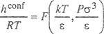
where σ and ε are characteristic size and energy parameters and where F is a function determined from experimental pure-component properties. To find h^conf(1) we assume

(7-113)

where F is the same function as in Eq. (7-112) and ε⁽¹⁾ and σ⁽¹⁾ denote composition averages for cells of type 1. For example, we might assume that

(7-114)

(7-115)

where ε_ij and σ_ij are constants characteristic of the i-j interaction. Similarly,

(7-116)

and, using the same assumption,

(7-117)

(7-118)

The molar configurational enthalpy of the mixture is given by Eq. (7-111); it is

(7-119)

The two-fluid theory for a binary mixture can be extended to mixtures containing any number of components. If there are m components, then there are m types of cells and the two-fluid binary theory becomes an m-fluid theory for an m-component mixture.

The UNIQUAC equation, proposed by Abrarns (1975), has been derived by Maurer (1978) using phenomenological arguments based on a two-fluid theory. This method is similar to that used by Renon (1969) in the derivation of the three-parameter Wilson equation. Maurer’s derivation avoids those inconsistencies that arise when a lattice one-fluid theory is used to derive UNIQUAC or any similar local-composition equation. The essential step in Maurer’s derivation is the adoption of Wilson’s assumption that local compositions can be related to overall compositions through Boltzmann factors.

We consider a binary mixture of molecules of components 1 and 2, where molecules 1 and 2 have arbitrary size and shape. As discussed in Sec. 6.11, molecules of component 1 consist of r₁ segments and each molecule has an external surface area proportional to q₁ Similar parameters are defined for molecules of component 2. For unisegmental (small, spherical) molecules, r = q = 1; for chain molecules, q/r < 1, but as the number of chain segments becomes large, q/r approaches a constant near 2/3.

For a polysegmented molecule i, the number of neighboring segments (belonging to other molecules) is zq_i where z is the coordination number.

To fix ideas, consider first a unisegmental molecule (r = q = 1). Suppose one molecule of component 1 is isothermally vaporized from its pure liquid denoted by superscript (0) and then condensed into the center of a cell as shown in the left side of Fig. 7-13 [hypothetical fluid (1)]. In this case, r =q =I also for molecules of component 2. A molecule 1 in the pure liquid has z⁽⁰⁾ nearest neighbors. Since intermolecuiar forces are short range, we assume pairwise additivity neglecting all except nearest neighbors; the energy of vaporization per molecule is where characterizes the potential energy of two nearest neighbors in pure liquid 1.

The central molecule in hypothetical fluid (1) is surrounded by z⁽¹⁾θ₁₁ molecules of species 1 and z⁽¹⁾θ₂₁ molecules of species 2, where θ₁₁ is the local surface fraction of component 1, about central molecule 1, and θ₂₁ is the local surface fraction of component 2, about central molecule 1 (note that θ₁₁ + θ₂₁= 1). We now assume that z₍₁₎ is the same as z⁽⁰⁾. The energy released by the condensation process is , where we have dropped the superscript on z. We make a similar transfer for a molecule 2 from the pure liquid, denoted by superscript (0), to a hypothetical fluid, denoted by superscript (2).

If we consider a mixture consisting of x₁ moles of hypothetical fluid (1) and x₂ moles of hypothetical fluid (2), the configurational part of an extensive property M of that mixture is given by Eq. (7-111). In particular, the total change in energy in transferring x₁ moles of species 1 from pure liquid 1 and x₂ moles of species 2 from pure liquid 2 into the “two-liquid” mixture, i.e., the molar excess energy u^E, is given by

(7-120)

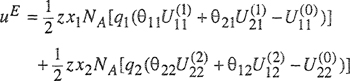
where N_A is Avogadro’s constant. Because the local surface fractions mast obey the conservation equations

(7-121)

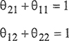
and assuming that and , Eq. (7-120) simplifies to

(7-122)

where we have now dropped the superscripts. Following Wilson (1964), we now assume

(7-123)

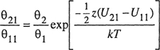
and

(7-124)

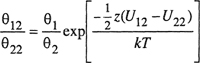
where θ is the surface fraction:

(7-125)

When these assumptions are coupled with Eq. (7-121), we obtain

(7-126)

and

(7-127)

(7-128)

where

(7-129)

Equation (7-126) is the fundamental relation based on two-fluid theory, utilizing the notion of local composition.

To obtain an expression for the molar excess Helmholtz energy, we use (at constant volume and composition),

(7-130)

where a^E is the excess Helmholtz energy per mole of mixture.

Integrating from 1/T₀ to 1/T, we have

(7-131)

We evaluate the constant of integration by letting 1/T₀→0. At very high temperature, we assume that components 1 and 2 form an athermal mixture (compare Sec. 8.2). As our boundary condition, we use the equation of Guggenheim (1952) for athermal mixtures of molecules of arbitrary size and shape,

(7-132)

where

(7-133)

Assuming that Δu₂₁ and Δu₁₂ are independent of temperature and that, as shown by Hildebrand and Scott (1950), at low pressures (a^E)_T,V ≈ (g^E)_T,P, Eq. (7-131) gives

(7-134)

where

(7-135)

(7-136)

that is the UNIQUAC equation.

As discussed in Sec. 6.11, Eq. (7-134) gives a good empirical representation of excess functions for a large variety of liquid mixtures. For mixtures containing more than two components, Eq. (7-134) can readily be generalized (Abrams and Prausnitz, 1975) without additional assumptions; the general result contains only pure-component and binary parameters.

While UNIQUAC has considerable empirical success, molecular-dynamic calculations suggest that the nonrandomeess assumption [Eqs. (7-123) and (7-124)] is too strong; the magnitudes of the arguments of the Bolt/mann factors are too large. In other words, UNIQUAC over-corrects for deviations from random mixing. While the basic ideas of UNIQUAC are useful, it is clear that significant modifications in the details are required to provide UNIQUAC with a sound molecular basis.¹⁶

¹⁶ J. Fischer and F. Kohler, 1983, Fluid Phase Equilibria, 14: 177; Y. Hu, E. G. Azevedo, and J. M. Prausnitz,1983, ibid., 13: 351; K. Nakanishi and H. Tanaka, 1983, ibid., 13: 371; and D. J. Phillips and J. F. Brennecke, 1993, Ind. Eng. Chem. Res., 32: 943.

7.8 Activity Coefficients from Group-Contribution Methods

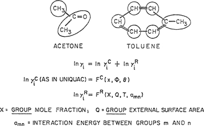
For engineering purposes, it is often necessary to make some estimate of activity coefficients for mixtures where only fragmentary data, or no data at all, are available. For vapor-liquid equilibria, such estimates can be made using a group-contribution method as illustrated in Fig. 7-14. A molecule is divided (somewhat arbitrarily) into functional groups. Molecule-molecule interactions are considered to be properly weighted sums of group-group interactions. Therefore, for a multifunctional component in a multicomponent system, group-contribution methods assume that each functional group behaves in a manner independent of the molecule in which it appears. Once quantitative information on the necessary group-group interactions is obtained from reduction of experimental data for binary systems, it is then possible to calculate molecule-molecule interactions (and therefore phase equilibria) for molecular pairs where no experimental data are available. The fundamental advantage of this procedure is that when attention is directed to typical mixtures of nonelectrolytes, the number of possible distinct functional groups is much smaller than the number of distinct molecules or, more directly, the number of distinct group-group interactions is very much smaller than the number of possible distinct molecule-molecule interactions.

Calculation of activity coefficients from group contributions was suggested in 1925 by Langmuir, but this suggestion was not practical until a large database and readily accessible computers became available. A systematic development known as the ASOG ¹⁷ (analytical solution of groups) method was established by Derr and Deal, (1969, 1973).

¹⁷ Parameters for the ASOG method are listed by K. Tochigi, D. Tiegs, J. Gmehling, and K. Kojima, 1990, J. Chem. Eng. Japan, 23: 453.

Figure 7-14 Activity coefficients from group contribution illustrated for a mixture of acetone and toluene. Acetone has two groups and toluene has six, as shown. For a component i, activity coefficient γ_i consists of two contributions, γ_i^c and γ_i^R where superscript C stands for configurational and superscript R stands for residual. Here F^C is a specified function of molecular composition and structure: moie fraction x, volume fraction Φ and surface fraction θ P^R is a specified function of group composition, structure and interaction energies: X, Qand a_mn. Both functions F^C and F^R are obtained from the UNIQUAC model. The key parameters are the group-group interaction parameters for ali pairs of groups (n,m) in the solution. In UNIFAC, for each pair, we use two parameters: a_mn and a_nm

A similar but more convenient method,¹⁸ based on the UNIQUAC equation, was developed fay Fredenslund, Jones and Prausnitz (1975) and discussed fay Fredensiund et al. (1977); this method, called UNIFAC (universal functional activity coefficient), is described in a monograph by Fredenslund et al. (1977a), but since its publication, numerous modifications and extensions have appeared (Fredenslund and Rasmussen, 1985; Gmehling, 1986; Larsen et al., 1987). A large number of group-group interaction parameters is available (Skold-JØrgensen et al. 1979; Macedo et al. 1983; Hatisen et al. 1991; Gmehling et al., 1993; Fredenslund and SØrensen, 1994); as new experimental data are reported, this number will rise. UNIFAC has been successfully used for the design of distillation columns (including azeotropic and extractive distillation) where the required multicomponent activity coefficients were estimated because of a lack of experimental information.

¹⁸ A comprehensive comparison between the predictive capabilities of ASOG and UNSFAC methods is presented by J. Gmehling, D. Tiegs, and U. Knipp, 1990, Fluid Phase Equilibria, 54:147.

Separate UNIFAC correlations have been proposed for liquid-liquid equilibria (Magnussen et al., 1981; Gupte and Daaner, 1987; Hooper et al., 1988), but these tend to be less accurate than those for vapor-liquid equilibria and, therefore, are not used widely. Some details concerning group-contribution methods (including correlations for polymer-solvent systems) and some other methods for estimating activity coefficients are briefly discussed in App. F.

For engineering design, correlations (in particular, group-contribution methods) are attractive because it is almost always easier and faster to make a calculation than to perform an experiment. However, because UNIFAC (and similar methods) frequently provide only rough approximations, it is often necessary to obtain at least a few reliable experimental results, either from the literature or from the laboratory. On the other hand, many experimental results reported in the literature are of poor quality and in that event, a calculated activity coefficient may be more reliable. There is no substitute for judgment. Users of correlations are privileged but they must also be cautious.

7.9 Chemical Theory

The models described in the previous sections attempt to explain solution nonideality in terms of physical intermolecular forces. These models relate the activity coefficients to physical quantities that reflect the size of the molecules and the physical forces (primarily London dispersion forces) operating between them. An alternate approach to the study of solution properties is based on a different premise, viz., that molecules in a liquid solution interact with each other to form new chemical species and that solution nonideality, therefore, is a consequence of chemical reactions.

We can distinguish between two types of reactions, association and solvation. Association refers to formation of chemical aggregates¹⁹ or dimers, trimers, etc. consisting of identical monomers. An association can be represented by reactions of the type

¹⁹ While aggregates are loosely bonded chemical compounds, this does not imply that they can necessarily be separated and exist by themselves. Such separations are possible only for stable compounds. The aggregates discussed here are often insufficiently stable for isolated existence.

where B is the monomer and n is the degree of association (or polymerization). A common case of association is dimerization (n= 2); a well-known example is dimerization of acetic acid:

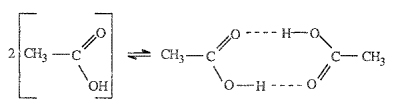
In this case, dimerization is due to hydrogen bonding that is responsible for the most common form of association in liquid solutions.

Salvation refers to formation of chemical aggregates of two or more molecules that are not all identical, represented by the general equation

A well-known example (n = m= 1) is solvation of chloroform and diethyl ether:

In this case, formation of the new species is again due to hydrogen bonding.

Another example of solvation is given by a charge-transfer complex between nitrobenzene and mesitylene:

In this case, a weak chemical bond is formed because mesitylene is a good electron donor (Lewis base) and nitrobenzene is a good electron acceptor (Lewis acid).

The chemical theory of solutions postulates existence of chemically distinct species in solution that are assumed to be in chemical equilibrium. In its original form, the theory then assumes that these chemically distinct substances form an ideal solution. According to these assumptions, the observed nonideality of a solution is only an apparent one because it is based on an apparent, rather than a true, account of the solution’s composition.

The chemical theory of solutions was first developed by Dolezalek (1908) at about the same time van Laar (1910) was publishing his work on solutions. The different points of view represented by these early workers in solution theory caused them to be hard enemies and some of their publications contain much bitter polemic.

Dolezalek’s theory has the advantage that it can readily account for both positive and negative deviations from ideality for molecules of similar size; also, unlike the van Laar-Scatchard-Hildebrand theory of regular solutions, it is applicable to mixtures containing polar and hydrogen-bonded liquids. Its great disadvantage lies in its arbitrariness in deciding what “true” chemical species are present in the solution, and in our inability to assign equilibrium constants to the postulated equilibria without experimental data on the solution under consideration. The chemical theory of solutions, therefore, has little predictive value: it can almost never give quantitative predictions of solution behavior from pure-component data alone. However, for those solutions where chemical forces are dominant, the chemical theory has much qualitative and interpretative value; if some data on such a solution are available, they can often be interpreted along reasonable chemical lines and, therefore, the chemical theory can serve as a tool for interpolation and cautious extrapolation of limited data. A chemical rather than a physical view is frequently useful for correlation of solution nonidealities in a class of chemically similar mixtures (e.g., alcohols in paraffinic solvents). In the next two sections, we discuss the properties of associated solutions. Solvated solutions are discussed in Secs. 7.12 and 7.13.

7.10 Activity Coefficients in Associated Solutions

Suppose we have a liquid mixture of two components, 1 and 2. Component 1 is a nonpolar substance that we designate A, but component 2 is a polar substance that we designate B and that, we assume, can dimerize according to

The equilibrium constant for this dimerization is given by

(7-137)

where a_B is the activity of monomer B molecules and a_B2 is the activity of dimer B₂ molecules.

We assume that species B and B₂ are in equilibrium with one another and we also assume that species A, B, and B₂ form an ideal liquid solution. In an ideal solution the activities can be replaced by the mole fractions and Eq. (7-137) becomes

(7-138)

where stands for the “true” mole fraction.

If there are n₁ moles of component 1 and n₂ moles of component 2, then

(7-139)

and

(7-140)

where n_B is the number of moles of monomer B and n_B2 is the number of moles of dimer B₂. The “true” total number of moles is n_A+n_B+n_B2 equal to n₁+n₂ – n_B2 The three “true” mole fractions are

(7-141)

(7-142)

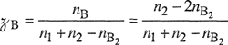
(7-143)

If we combine Eq. (7-138) with Eqs.(7-142) and (7-143) and then eliminate n_B2 with Eq. (7-141), we obtain an expression that we can solve for and from this we can obtain the desired result for the activity coefficient of component 1. The algebra is straightforward but involved, and is not reproduced here. Remembering that X₁=n₁/(n₁+n₂) and that X₂=n₂/(n₁+n₂), we obtain

(7-144)

where k ≡ 4K + 1

By similar stoichiometric considerations, the activity coefficient for the dimerizing component can be shown to be²⁰

²⁰ Appendix G presents the genera! relation for associated and solvated mixtures. It is shown there that the chemica! potential of a (stoichiometric) component is equal to that of the component’s monomer.

(7-145)

Figure 7-15 shows plots of Eqs.(7-144) and (7-145) for three dimerization equilibrium constants. It is a property of both Eqs. (7-144) and (7-145) that for all K > 0, positive deviations from Raoult’s law result; thus γ₁≥1 and γ₂≥1, as shown. For K = ∞ all molecules of component 2 are dimerized; in this limiting case we have

(7-146)

Figure 7-15 Activity coefficients of a dimerizing component (2) and an “inert” solvent (1).

At infinite dilution,

(7-147)

For the nondimerizing component, the largest possible value of γ₁ is 2.

To test the dimerization model represented by Eqs. (7-144) and (7-145), we can compare calculated and observed activity coefficients for a binary system containing an organic acid in a nonpolar “inert” solvent because spectroscopic, cryoscopic, and distribution data indicate that organic acids have a strong tendency to dimerize. Figure 7-16 shows a comparison for propionic acid dissolved in n-octane. Because the experimental data (Johnson et al., 1954) were unfortunately obtained at constant pressure rather than constant temperature, the comparison is not completely straightforward because the dimerization equilibrium constant depends on temperature.

Figure 7-16 Calculated and experimental activity coefficients for propionic acid (2) dissoived in n-octane (1) at 1.013 bar (temperature between 121.3 and 141.1°C).

The experimental data shown in Fig. 7-16 follow the general trend predicted by Eq.(7-145), but even with K = ∞, the observed deviations from ideality are larger than those calculated. Because dimerization of an organic acid is exothermic, dimerization constant K falls with rising temperature but it is apparent that the variable temperature of the experimental data is not responsible for the lack of agreement between theoretical and experimental results. In this case, the chemical theory is evidently able to account qualitatively for the observed activity coefficients but, because physical effects are neglected by the chemical theory, quantitative agreement is not obtained.

Another comparison between calculated and experimental results, given in Fig. 7-17, shows activity coefficients for acetic acid in the benzene/acetic acid system at 25°C. Experimental data were reported by Hovorka and Dreisbach (1934) and, again, qualitative agreement is obtained between experimental and theoretical results.²¹ The activity coefficients for acetic acid in benzene are somewhat lower than those for propionic acid in octane; because of the higher polarizability of π electrons in benzene, it is likely that the forces of attraction between benzene and acid are stronger than those between octane and acid.

Figure 7-17 Calculated and experimental activity coefficients for acetic acid (2) dissolved in benzene (1) at 25°C.

²¹ Figure 7-17 presents two sets of results, each based on a particular method of data reduction. Because total pressure at 25°C is much less than 1 bar, activity coefficients represented by triangles were calculated from the experimental data without any vapor-phase correction; neither the fugacity of the acid in the vapor-phase mixture nor the (standard- state) fugacity of pure acetic acid were corrected for nonideal behavior. However, as discussed in Sec.5.9, vapor-phase corrections are important for carboxylic acids even at pressures of the order of 10^-2 bar. When such corrections are included in data reduction, the results obtained are those represented by circles.

The two examples given in Figs. 7-16 and 7-17 show only fair agreement between theory and experiment. But even if the agreement were good, it should not by itself be considered proof of the validity of the chemical theory. Good agreement would have shown only that the assumptions of the chemical theory, with the help of one adjustable parameter, are consistent with the experimental facts, but the assumptions of some other theory, again with one adjustable parameter, may be equally consistent with these facts. In other words, when agreement is good, we may say that the chemical theory offers a possible, but by no means unique, explanation of the observed thermodynamic properties. A chemical theory of solution behavior must always be viewed with suspicion unless there is independent evidence to support it. In the case of propionic (or acetic) acid, dissolved in octane or some other relatively “inert” solvent, we believe that the chemical explanation is reasonable because of independent (e.g., spectroscopic and cryoscopic) evidence That evidence strongly supports the assumption that organic acids do, in fact, dimerize in nonpolar solvents.

In Eq. (7-144), even, a very large values of the dimerization equilibrium constant K cannot produce high activity coefficients for the “inert” component; yet, such activity coefficients have been observed in some associated solutions, notably for nonpolar solvents dissolved in an excess of alcohol. Further, the activity coefficients of the associating component are often considerably larger than those calculated by Eq. (7-145) with K = ∞. To explain these very large activity coefficients, it has been proposed that the associating component undergoes chain association; i.e., it forms not only dimers but also trimers, tetramers, etc., according to

2B B₂

B + B₂ B₃

B + B₃ B₄ etc.

For example, phenol is known from a variety of physicochemical data to form a multiple chain according to the structure

Because the tendency of phenol to form chains is a strong function of phenol concentration (especially in the dilute region), it follows that the activity of phenol, when dissolved in some solvent, shows large deviations from ideal behavior (Tucker and Christian, 1978).

The thermodynamics of solutions that contain a component capable of multiple association has been considered by many authors; good discussions of this subject are given by Kortiim and Buchholz-Meisenheimer (1952), by Prigogine and Defay (1954), and by Tucker and Lippert (1976). We discuss here only the main concepts and present some typical results.

To reduce the number of adjustable parameters, it is common to assume that the equilibrium constant for the formation of a chain is independent of the chain length. That is, if we write the general association equilibrium

B + B_n-1 B_n

then the equilibrium constant K_n is

(7-148)

where a is the activity. The simplifying assumption is that K₂ = K₃ = ... = K_n = K.²²

²² Studies have been reported where this assumption is not made (Tucker and Lippert, 1976). However, the algebraic complexity and the amount of data required for meaningful data reduction are much iarger when the equilibrium constant is allowed to depend on the degree of association and frequently the extra labor is not justified. One fine example, however, of such a detailed study is that by H. Wolff and A. Höpfner (1962, Z. Elekirochem., 66: 149) for solutions of methylamine and hexane. These authors, using extensive data for the range -55 to 20°C, report equilibrium constants and enthalpies of formation for dimes, trimers, and teiramers of raethylamine. At a given temperature, the authors found that the three equilibrium constants are close but not identical.

If, as before, we assume that the solution of “true” species is an ideal solution, then we can replace activity a by “true” mole fraction . The mathematical details are tedious and not reproduced here, but it can be shown that the activity coefficient of component 2, the associating component, is given by

(7-149)

where

(7-150)

The activity coefficient of the nonassociating component 1 is given by

(7-151)

Figure 7-18 shows activity coefficients for the multiply-associated component for several values of equilibrium constant K. At small mole fractions, the activity coefficients are now much larger than those shown in Fig. 7-15 that considered only dimerization. The activity coefficients for the associated component are large at the dilute end but fall rapidly as the concentration rises; this characteristic behavior is in excellent agreement with experimental results for solutions of alcohols in nonpolar solvents. For example, Prigogine et al. (1949, 1951) have shown that observed excess Gibbs energies of solutions of alcohols in carbon tetrachloride can be closely approximated by ascribing the nonideality of these solutions to multiple association. The small difference between calculated and observed excess Gibbs energies is probably due to physical forces that, by assumption, have been neglected in this purely chemical treatment. We shall return to this point in the next section, but first we want to consider some of the implications of the chemical theory of associated solutions.

Figure 7-18 Activity coefficients of a multiply-associated component in an “inert” solvent.

When considering the validity of any theory of solutions, it is important to inquire whether or not it can be supported by evidence based on several physicochemical properties. The validity of any theory of solution is much enhanced if it can be shown to be in agreement with observed physical properties other than those used to obtain activity coefficients. For the theory of associated solutions, where association is due to hydrogen bonding, such support is provided by infrared spectroscopy as shown by many workers, notably by Hoffmann, Errera, Sack, and others (see Tucker and Lippert, 1976; Pimentel and McClellan, 1960). For example, consider a solution of methanol in a nonpolar solvent such as carbon tetrachloride. The frequency of vibration of the OH group is in the infrared spectrum and this frequency is strongly affected by whether or not it is “free” (i.e., attached only to a carbon atom by a normal covalent bond) or whether it is also attached to another OH group through hydrogen bonding. Therefore, by measuring the intensity of absorption at the frequency corresponding to this “free” vibration, it is possible to determine the concentration of alcohol that is in the monomeric, nonassociated state. Spectroscopic measurements thus provide an independent check on the theory of associated solutions.

If we let α_B1, stand for the fraction of alcohol molecules in the monomeric form, then, as shown by Prigogine, we can relate α_B1 to the unsymmetrically normalized activity coefficients of alcohol (2) and carbon tetrachloride (1) by the remarkably simple equation

(7-152)

where ϒ₂^* and ϒ₁ are activity coefficients normalized by the unsymmetric convention (see Sec. 6.4):

Figure 7-19 compares values of α_B1 determined spectroscopically, with those determined by standard thermodynamic measurements for the system methanol/carbon tetrachloride. The good agreement lends support to the essential ideas of the theory of multiple association for mixtures of alcohols and nonpolar solvents; however, studies by Van Ness el al. (1967) and Nagata (1977, 1978) indicate that the structure of alcohol solutions is probably considerably more complex than that assumed by Prigogine.

The simple theory of multiply-associated solutions (Kortiim and Buchholz-Meisenheimer, 1952), also establishes a relation between the activity coefficient of the nonassociating solvent and , the average chain length of the associating component:

(7-153)

Figure 7-19 Fraction of monomeric methanol molecules in carbon tetrachloride solution at 20°C.

A comparison can then be made between average chain lengths calculated from activity coefficients and from other physicochemical measurements such as spectroscopy and cryoscopy. Again, good agreement is often obtained when results based on different methods of measurement are compared with one another.

Figure 7-20 shows average chain lengths as a function of alcohol concentration for several systems (Mecke, 1948). The degree of association rises rapidly in the dilute region; this is consistent with the experimental observation that the activity coefficient of an alcohol in a nonpolar solvent is large at infinite dilution but then falls quickly as the mole fraction of alcohol rises.

Figure 7-20 Average chain length of multiply-associated solutes in various solvents, as determined by infra-red spectroscopy (Mecke, 1948).

Figure 7-20 shows that for phenol in carbon tetrachloride, the extent of association falls with rising temperature, as expected, because the association reaction (hydrogenbonding) is exothermic. However, Fig. 7-20 also shows that for phenol at a constant temperature of 20°C, the average chain length depends not only on the alcohol concentration but also on the nature of the solvent.²³ This observation is not consistent with the assumptions of the chemical theory that postulates that the role of any solvent is merely that of an inert dispersing agent for the associated component; in other words, the chemical theory assumes that solvent-solute interactions make no contribution to solution nonideality. According to the theory of multiple association, at a fixed temperature, the activity coefficient of an associating component should be a function only of its mole fraction regardless of the nature of the “inert” solvent. However, experimental data for many solutions of alcohols in nonpolar solvents show that this is not the case, indicating that the concept of an inert solvent is a convenient, but unreal oversimplification,

²³ Notice that for phenol is significantly lower in chlorobenzene and benzene than in carbon tetrachloride. This result is probably due to soivation between the alcohol and the π-electrons of the aromatic solvents.

7.11 Associated Solutions with Physical Interactions

The chemical solution theory of Dolezalek assumes that all deviations from ideal behavior are due to formation and decomposition of chemical species and that once the mole fractions of the true species are known, the properties of the solution can be calculated without further consideration to interactions between the true species. By contrast, the physical theory states that the true species are the same as the apparent species and that while there are physical (van der Waals) intermolecular forces, there are no chemical reactions in the solution.

The chemical and the physical theories of solutions are extreme, one-sided statements of what we now believe to be the correct situation. In certain limiting cases, each theory provides a satisfactory approximation: When forces between molecules are weak, no new stable chemical species are formed and the physical theory applies; on the other hand, when forces between molecules are strong, these forces result in the formation of chemical bonds; because the energies for chemical bond formation are significantly larger than those corresponding to van der Waals forces,²⁴ the chemical theory for such cases provides a reasonable description. In general, both physical and chemical forces should be taken into account. A comprehensive theory of solutions should allow for a smooth transition from one limit of a “physical” solution, to the other limit of a “chemical” solution.

²⁴ Roughly speaking, weak forces between molecules are those that have energies less than RT, while strong forces between molecules are those whose energies are considerably larger than RT. At room temperature RT is about 2500 J mol^-1.

It is difficult to formulate a theory that takes into account both physical arid chemical effects without thereby introducing involved algebra and, what is worse, a large number of adjustable parameters. Nevertheless, a few attempts have been made and one of the more successful is based on the theory of polymer mixtures by Flory (1944). This theory has been applied to mixtures containing aliphatic alcohols and paraffinic hydrocarbons (Scatchard, 1949; Kretschmer and Wiebe, 1954; Smith and Brown, 1973); in such mixtures, alcohol polymerizes to form chains, but these chains interact with the paraffin only through van der Waals forces. We now briefly outline the essential ideas of the theory of associated solutions following the discussion of Renon (1967).

Let A stand for the hydrocarbon and B for the alcohol. We assume that:

1. The alcohol exists in the solution in the form of linear, hydrogen-bonded polymers B1, B2,…, Bn,…, formed by successive reactions of the type

B + B_n-1 B_n

2. The association constant for the reaction above is independent of n.

3. The molar volume of an n-mer is given by the molar volume of the monomer multiplied by n.

4. There are physical interactions between all molecules. These lead to contributions to liquid-mixture nonideality that can be described by expressions of the van Laar form.

5. The temperature dependence of the association constant K is such that the enthalpy of formation of a hydrogen bond is independent of temperature and degree of association.

On the basis of his lattice model, Flory (1944) derived expressions for the thermodynamic properties of solutions of polymers differing only in molecular weight; these expressions are especially suited for chemical equilibria between linear, polymeric species. We can use Flory’s results for the entropy of mixing to obtain the proper expression for the equilibrium constant. It is

(7-154)

where Φ_Bn is the volume fraction of species B_n.

The derivation of Eq.(7-154) is given elsewhere (Flory, 1944). Flory’s result clearly shows that the equilibrium constant should not be expressed in terms of mole fractions as in Sec.7.10.

As shown by several authors (Scatchard, 1949; Kretschmer and Wiebe, 1954; Smith and Brown, 1973; Renon and Prausnitz, 1967; Redlich and Kister, 1947), the excess Gibbs energy, taken relative to an ideal solution of alcohol and hydrocarbon, can be separated into two contributions, one chemical and the other physical:

(7-155)

The chemical contribution g_c^E results from the dependence of the “true” composition of the solution on the chemical equilibria indicated by assumption 1. The excess entropy introduced by mixing of polymeric species is taken into account in the calculation of the chemical contribution. From Flory’s theory we have

(7-156)

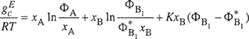
where x_A and x_B are the overall (stoichiometric) mole fractions. Φ_B1 is the (true) volume fraction of molecular species B₁, the alcohol monomer, and

We can obtain Φ_B1Bl from the equilibrium constant:

(7-157)

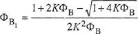
where Φ_B is the overall volume fraction of alcohol. The volume fraction of alcohol monomer in pure alcohol then becomes

(7-158)

The physical contribution g_p^E is given by a one-parameter equation as suggested by Scatchard (1949):

(7-159)

where ß is a physical interaction parameter related to the hydrocarbon-alcohol monomer interaction, υ_A and υ_B are liquid molar volumes.

Activity coefficients and the enthalpy are found by appropriate differentiation. The results are:

(7-160)

(7-161)

(7-162)

(7-163)

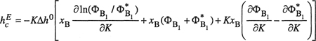
(7-164)

where

(7-165)

and Δh^o is the molar enthalpy of hydrogen-bond formation.

For the Gibbs energy of any alcohol/hydrocarbon system at a fixed temperature, the theory requires only one physical interaction parameter β and one equilibrium constant K. The equilibrium constant, however, depends only on the alcohol and is independent of the hydrocarbon solvent.

Renon’s reduction for 11 binary alcohol/hydrocarbon systems is typically represented by Figs. 7-21 and 7-22. Considering the totality of the data, Renon chose only one value for Δh⁰, i.e., -25.1 kJ mol^-1. This value fixes the temperature dependence of K for all alcohols according to

(7-166)

Figure 7-21 Excess functions for methanol/n-hexane mixtures. Here stands for the physical (as opposed to chemical) contribution to the excess enthalpy.

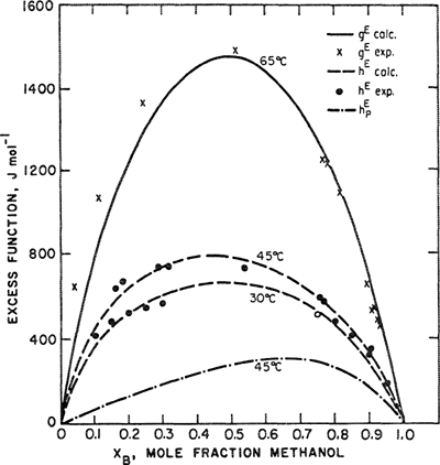
Figure 7-22 Excess functions for ethanol/n-hexane mixtures. Here stands for the physical (as opposed to chemical) contribution to the excess enthalpy.

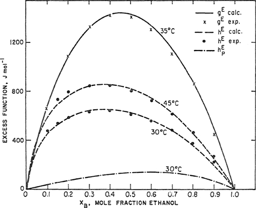
Each alcohol is further characterized by the value of K at one temperature. At 50°C, K is 450 for methanol, 190 for ethanol, 60 for isopropanol, and 90 for n-propanol.²⁵ These constants were obtained upon considering the totality of the data for each alcohol, but giving more weight to the more sensitive data (enthalpies) in the region where the model is physically most reasonable, i.e., at low temperatures and at high alcohol concentrations.

²⁵ Other values for K have been suggested. See, for example, A. Nath and E. Bender, 1981, Fluid Phase Equilibria, 7: 275, 289.

Renon’s data reduction indicates that the theory described gives a good representation of the experimental data in accord with the physical meaning of the model. Discrepancies become large only where the degree of alcohol polymerization is small, i.e., at low alcohol concentrations and at higher temperatures. A particularly sensitive test of the theory is provided by comparison of calculated and experimental results for excess enthalpies at several temperatures.

In spite of its simplifying assumptions, the Flory-Scatchard model of associated solutions gives a good representation of the properties of concentrated solutions of alcohols in saturated hydrocarbons. It probably takes into account the major effects, but perhaps neglects others, such as formation of cyclic polymers.

The theory just described can be extended to include other chemical effects such as, for example, solvation between solute and solvent, or even association of both components, each with itself and with the other. For each assumed chemical equilibrium, a characteristic equilibrium constant must be introduced and thus a more general treatment, including various types of chemical equilibria, results in complicated algebraic expressions and, what is worse, requires a large number of empirical parameters.

Numerous models have been developed for solutions containing associating molecules making use of the idea to separate thermodynamic excess properties into a chemical and a physical contribution. They differ from each other with respect to the particular expressions used for the two contributions. Using the same basic ideas for the chemical contribution as discussed above, such models are, e. g., the dispersivequasi-chemical (DISQUAC) model proposed by Kehiaian (1983, 1985), the extended-real-associated-solution (ERAS) model developed by Heintz (1985), the lattice-fluid-association (LFAS) model of Panayiotou (1988, 1991), and the model proposed by Nagata et al. (1997). All these models have been used to describe phase equilibria and thermodynamic excess properties. For example, recent variations include the DISQUAC model by González (1997, 1997a), the LFAS model by Ormanoudis and Panayiotou (1993), and the ERAS model by Heintz and Papaioannou (1998) and Kammerer et al. (1998). However, with these models, phase equilibria and excess properties usually cannot be described simultaneously using the same model parameters.

A more fundamental method to account for association and/or solvation is the statistical associated-fluid theory (SAFT) developed by Chapman et al. (1989, 1990). The SAFT equation of state has been successfully used to model phase behavior and thermodynamic properties for a large variety of simple and complex fluid and fluid mixtures. SAFT is discussed in Sec. 7.17.

We must recognize that the distinction between chemical and physical contributions to the excess Gibbs energy leads to an arbitrary and, perhaps, artificial model based on a simplified picture of solution properties. The designation of molecular interactions as either chemical or physical is only a convenience that probably cannot be justified by a sophisticated modern theory of intermolecular forces. Nevertheless, a joint chemical and physical description of equilibrium properties of mixtures, as exemplified by Eqs. (7-160) and (7-161), provides a reasonable and useful description for highly nonideal solutions that is a considerable improvement over the idea! chemical theory of Dolezalek on the one hand and the purely physical theory of van Laar on the other.²⁶

²⁶ A fine study incorporating both chemical and physical effects has been presented by Calado and Staveley, 1979.Fluid Phase Equilibria, 3: 153, who correlated vapor-liquid equilibrium data for the system NO/Kr at 115.76 K. In this system there is appreciable dimerization of NO to (NO)₂,.

7.12 Activity Coefficients in Solvated Solutions

The chemical theory of solutions has frequently been used to describe thermodynamic properties of binary solutions where two components form complexes. There are many experimental studies of such solutions that, if the complex is stable enough, are characterized by negative deviations from Raoult’s law. To illustrate, we consider first a simple case, a binary solution where complexes form according to

(7-167)

The equilibrium constant K is related to the activities of the three species by

(7-168)

If the solution is formed from n₁ moles of A and n₂ moles of B, and if at equilibrium, n_AB moles of complex are formed, the true mole fractions A, B, and AB are

(7-169)

(7-170)

(7-171)

Following Dolezalek, we assume that the true species form an ideal solution and therefore the activity of each species is equal to its true mole fraction. Equations (7-168) to (7-171) may then be used to eliminate n_AB. The apparent mole fractions of the two components are x₁ (for A) and x₂ (for B). They are given by

Algebraic rearrangement then gives for the activity coefficients:

(7-172)

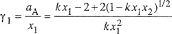
(7-173)

where k = 4K/(K + 1). Because of symmetry in Eq. (7-167), γ₁ depends on x₁ in exactly the same way as γ₂ depends on x₂.

Figure 7-23 shows γ₁ as a function of x_l for several values of equilibrium constant K. When K = 0, γ₁ = 1 for all as expected, because in that case no complex is formed, and therefore, by assumption, there is no deviation from ideal behavior. At the other extreme, when K = ∞, activity coefficients of both components go to zero at the midpoint (x₁ = x₂ = 1/2) because at this particular composition all molecules are complexed and no uncomplexed molecules A or B remain.

Figure 7-23 Activity coefficients of a solvating component that forms a bimolecular complex.

Equations (7-172) and (7-173) predict negative deviations from Raoult’s law for K > 0 and as a result, it has unfortunately become all too common immediately to ascribe observed negative deviations from Raoult’s law to solvation effects. It is true that strong negative deviations usually result from complex formation and conversely, if strong complexing is known to occur, negative deviations usually result. However, these conclusions are not always valid because they are based on a strictly chemical theory that neglects all physical effects. In systems where complexing is weak, physical effects are by no means negligible and as a result, weakly solvated solutions sometimes exhibit positive deviations from Raoult’s law. Also, small negative deviations from Raoult’s law may occur in the absence of complexing as has been observed, for example, in mixtures of normal paraffins, where differences in molecular size give positive excess entropy.

Equations (7-172) and (7-173) have been applied to a large number of solutions; one of these is the diethyl ether/chloroform system. Vapor-liquid equilibrium data for this system at several temperatures can be reduced using Eqs. (7-172) and (7-173) and the following equilibrium constants are then obtained:

Because the formation of a hydrogen bond between ether and chloroform is an exothermic reaction, we expect the equilibrium constant to fall with rising temperature, as indeed it does. From the equilibrium constants, we can calculate Δh⁰, the enthalpy of hydrogen-bond formation, and we find that for ether/chloroform, Δh⁰ is close to -12.5 kJ mol^-1, a reasonable value, in approximate agreement with those obtained by other experimental measurements.

Equations (7-172) and (7-173) have been derived for the case where the two components form a 1:1 complex. Similar equations can be derived for cases where the stoichiometry of the complex is 2:1, or 3:1, or 3:2, etc. This flexibility is both a strength and a weakness of the chemical theory of solutions. It is a strength because it can "explain" solution behavior for any sort of chemical interaction and therefore it has, potentially, a wide range of applicability. It is a weakness because, unless other information is available, the stoichiometry of the complex is another adjustable parameter, in addition to the equilibrium constant. Thus, if a particular assumed stoichiometry does not fit the experimental data, one can try another, and so on, and eventually a fit is obtained. Such a fit, however, has no physical significance unless there is independent evidence from the molecular structure of the components to verify the assumed stoichiometry. For diethyl ether/chloroform mixtures, it would be difficult to justify any complex other than one having a 1:1 stoichiometry.

As shown by Harris (1969), we can relax Dolezalek’s assumption that the "true" chemical species form an Idea! solution. Harris assumed that a mixture of "true" species is described by an equation of the van Laar type. For example, we again consider a mixture of molecules A and B that interact strongly to form complex AB:

(7-174)

Let K be the equilibrium constant for this chemical equilibrium and let A, B, and AB stand for the true mole fractions. Then

(7-175)

where γ’ stands for the true activity coefficient. Dolezalek assumed that all γ’ are equal to unity. Harris, however, makes the more reasonable assumption that for any true component k,²⁷

²⁷ For mixtures of components of greatly different size, improved representation of the true activity coefficients may be obtained by adding to the right-hand side of Eq. (7-176) the Flory-Huggins term: RT[la Φ/ _k + 1 - Φ/_k].

(7-176)

where Φ is the volume fraction:

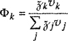
and where ν_i is the liquid molar volume of i and α_ij is a (van Laar) parameter for physical interaction of molecules i and j Subscripts i, j, and k are understood in this case to range over the three possible species A, B, and AB. Equation (7-176) contains three physical parameters: α_A-B, α_A-AB, and α_B-AB. To limit the number of adjustable parameters to two (one chemical parameter K and one physical parameter α), it is necessary to use plausible physical arguments for relating α_A-AB α_B-AB to α_A-B’ as described by Harris (1969).

To reduce experimental vapor-liquid equilibrium data with Eqs. (7-175) and (7176), we use a powerful theorem discussed in detail by Prigogine and Defay (1954) and summarized in App. G. It can be rigorously shown that for a mixture of components 1 (species B) and 2 (species A), the apparent activity coefficients and apparent mole fractions are related to the true activity coefficients and true mole fractions by

(7-177)

(7-178)

Equations (7-177) and (7-178) are independent of any physical model. They follow directly from the assumption that the “true” species A, B, and AB are in equilibrium.

For data reduction, Eqs. (7-175) to (7-178) must be combined with material balances relating true mole fractions to apparent mole fractions. This is done most conveniently in terms of the normalized extent of complex formation ξ(0 ≤ξ ≤1/2):

(7-179)

(7-180)

(7-181)

To illustrate Harris’ extension of Dolezalek’s theory, Fig. 7-24 gives results of data reduction for solutions of acetylene in three organic solvents. Acetylene forms hydrogen bonds with butyrolactone and N-methylpyrrolidone but not with hexane. To represent the experimental data for the two polar solvents, two parameters (K and α) are required, whereas the experimental data for hexane are represented with only one parameter, because K = 0. In hexane, a “physical” solvent, acetylene exhibits positive deviations from Raoult’s law over the entire composition range. In chemical solvents, however, acetylene exhibits negative deviations from Raoult’s law at the solvent-rich end and positive deviations at the acetylene-rich end. Dolezalek’s theory (with one chemical equilibrium constant) cannot account for such behavior. The modification of the chemical theory proposed by Harris combines into one comprehensive model the ideas of both Dolezalek and van Laar.²⁸

Figure 7-24 Calculated and observed activity coefficients for acetylene (2) in three organic solvents.

²⁸ An engineering-oriented study incorporating both solvation equilibria and physical effects was presented by Rivas, 1979, AIChE J., 25: 975, who correlated solubility data for CO₂ and H₂S in mixed solvents for sweetening of sour natural (or synthetic) gases.

7.13 Solutions Containing Two (or More) Complexes

The chemical theory can be extended in a straightforward way to the case where several complexes of different stoichiometry are formed by the two components. For the same reasons as those stated in the preceding section, this possibility for extension carries with it an advantage and a danger. The advantage lies in the gain in flexibility; the danger arises because if one postulates enough complexes, one necessarily introduces a sufficient number of adjustable parameters to fit any data for any system.

An excellent study of a binary solution that contains two types of complexes has been reported by McGlashan and Rastogi (1958) who investigated thermodynamic properties of the p-dioxan/chloroform system; p-dioxan is a symmetric cyclic ether containing two oxygen atoms and therefore McGlashan and Rastogi postulated the existence in solution of two complexes having the structures

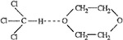
and

Let A stand for dioxan and B for chloroform. Two equilibria are postulated:

(7-182)

(7-183)

Two equilibrium constants are defined by

(7-184)

(7-185)

We assume that this (apparent) binary, nonideal solution is an ideal solution of four true components (A, B, AB, and AB2). The activity of each true component is then equal to its true mole fraction and Eqs. (7-184) and (7-185) become

(7-186)

(7-187)

By material balance,

(7-188)

Eliminating _AB and _AB2 with Eqs. (7-186) and (7-187), Eq. (7-188) becomes, after rearrangement,

(7-189)

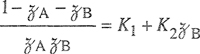
or

(7-190)

Activities a_A and a_B are obtained from experimental vapor-liquid equilibrium data.

A plot of the left side of Eq. (7-190) versus a_B should give a straight line whose intercept and slope yield the two equilibrium constants K₁ and K₂. Such a plot was constructed by McGlashan and Rastogi (1958) who found that at 50°C, K₁ = 1.11 and K₂ = 1.24.

Once numerical values are given for the two equilibrium constants, activity coefficients can be calculated as shown by McGlashan and Rastogi. The activity coefficient of B (chloroform) is given by

(7-191)

and the true mole fraction of B is related by material balances to x_B, the apparent mole fraction, by

(7-192)

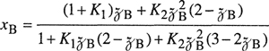
The activity coefficient of A (dioxan) is given by

(7-193)

Figure 7-25 gives a plot of calculated and observed activity coefficients. The excellent agreement shows that for this system calculations based on the assumption of the existence of two justifiable complexes can account for the system’s thermodynamic behavior.

Figure 7-25 Activity coefficients for a solvated mixture: p-dioxan/chloroform at 50ÄC (McGiashan and Rastogi, 1958).

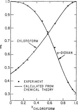
McGlashan and Rastogi also measured calorimetrically the enthalpy of mixing for this system. Using the chemical solution theory just described, the enthalpy of mixing can be related to the enthalpy of complex formation.

Because

(7-194)

and because

(7-195)

substitution of Eqs. (7-191) and (7-193) for γ_A and γ_B gives

(7-196)

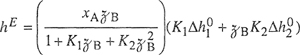
where is the enthalpy of formation of complex AB and is the enthalpy of formation of complex AB₂:

(7-197)

(7-198)

By fitting experimentally determined enthalpies of mixing to Eq. (7-196), the enthalpies of complex formation are

These are reasonable values; is the enthalpy of formation of one etheroxygen hydrogen bond and it agrees well with results determined by spectroscopic, cryoscopic, and other methods. The enthalpy of formation for the complex containing two hydrogen bonds is not quite twice that for the formation of one hydrogen bond. This is not surprising because the two oxygen atoms in dioxan are only separated by two carbon atoms; therefore, the effect of hydrogen bonding one oxygen atom has an appreciable effect on the other oxygen atom. If the two oxygen atoms were farther apart, one might expect that would be more nearly equal to 2.

7.14 Distribution of a Solute between Two Immiscible Solvents

The chemical theory of solution attempts to explain thermodynamic properties in terms of actual (true) chemical species present in solution. An explanation of this sort can sometimes be applied toward interpreting and extending data on partition coefficients for a solute between two immiscible liquid solvents. We present next one example illustrating such application (Moelwyn-Hughes, 1940).

Consider two liquid phases α and β; a solute, designated by subscript 1, is distributed between these two phases. First, we consider a simple case. Suppose that the mole fraction of solute in either phase is very small and that we can therefore assume the two solutions to be ideal dilute solutions. We then have

(7-199)

(7-200)

where H_1,α is Henry’s constant for solute 1 in phase a and H_1,β is Henry’s constant for solute 1 in phase β. Equating fugacities of component 1 in the two phases, we obtain the partition coefficient K,

(7-201)

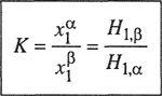
At constant temperature and pressure, for sufficiently dilute solutions, the partition coefficient in Eq. (7-201) is a constant, independent of composition. Equation (7-201) is frequently called the Nernst distribution law.

Because mole fractions and are very small, they are, respectively, proportional to the concentrations of solute 1 in phase α and in phase β it is therefore customary to use a somewhat different partition coefficient, K’, expressed in terms of concentrations c rather than mole fractions x:

(7-202)

where p^α and p^β are, respectively, the molar densities of phases α and β. For very small x₁, p^α and p^β are the densities of the pure solvents.

Many cases are known where the Nernst distribution law is not consistent with experiment, even though the solute mole fractions are small; in other words, in these cases, the equations for ideal dilute solutions [Eqs. (7-199) and (7-200)] are not obeyed in either (or both) of the liquid phases at the particular concentrations investigated.²⁹ In many cases, departure from Nernst’s law may be ascribed to chemical effects. We now consider such a case: the distribution of benzoic acid between the two (essentially) immiscible solvents water and benzene near room temperature. The explanation for the failure of Nernst’s law can, in this case, be found by taking into account the tendency of organic acids to dimerize in a nonpolar solvent.

²⁹ The ideal-dilute-solution equation is always approached for any nonelectroiyte when the mole fraction is sufficiently small, but just how small depends on the system. For a solute that associates in solution, it may be very small indeed, sometimes smaller than can be measured by common analytical methods.

We postulate two equilibria as shown in Fig. 7-26:

Figure 7-26 Distribution of benzoic acid between benzene and water.

1. Phase-distribution equilibrium between the two phases:

Acid in water monomer acid in benzene

2. Chemical equilibrium in the benzene phase:

Monomer acid dirner acid

For each equilibrium there is an equilibrium constant:

(7-203)

(7-204)

In Eqs. (7-203) and (7-204), c stands for concentration of benzoic acid; superscript B stands for the benzene phase and superscript W for the water phase. Subscript M stands for monomer and subscript D for dimer.³⁰

³⁰ In the dilute aqueous phase, benzoic acid is probably completely solvated by hydrogen bonding with water.

Let stand for the total concentration of benzoic acid in benzene. By material balance,

(7-205)

Substitution of Eqs. (7-203) and (7-204) into Eq. (7-205) gives the distribution law

(7-206)

In this case, then, the distribution coefficient (i.e., the ratio of to c^w) is not constant, as it would be according to Nernst’s law, but varies linearly with the concentration of benzoic acid in water. Experimental data for this system (Nernst, 1891) are plotted in Fig. 7-27 in the form suggested by Eq. (7-206). The straight line obtained confirms the prediction based on the chemical theory of solutions; from the slope and intercept k₁ = 1.80 (dimensionless) and K_II = 176 dm³ mol^-1. By plotting the data in this way, one can, using only a few experimental points, interpolate and slightly extrapolate with confidence.

Figure 7-27 Linearization of distribution data with chemical theory: the system benzoic acid/water/benzene at 20°c.

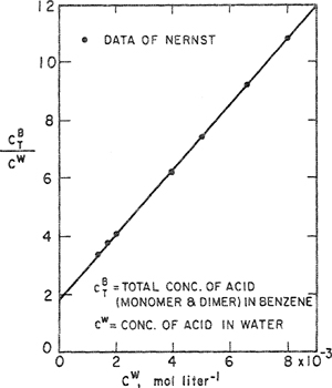
In some systems, where the tendency of the solute to dimerize is strong, K_II is very large. If, in the system just discussed, benzoic acid dimerized strongly, we would have

(7-207)

giving the distribution law

(7-208)

Various examples of this distribution law have been found. Whenever a system behaves according to Eq. (7-208), it is considered good evidence that the solute molecules

are strongly dimerized in one of the solvents. In the benzole acid/water/benzene system, dimerization of benzole acid is moderately strong but the inequality given in Eq. (7-207) is not valid until c^w is at least 10^-2 mol liter^-1.

An example of the applicability of Eq. (7-208) is given in Fig. 7-28. In both alkanoic acid/water/n-dodecane systems (Aveyard and Mitchell, 1970), nearly all acid molecules are dimers in n-dodecane.

Figure 7-28 Linearization of distribution data for two alkanoic acids distributed between water and n-dodecane at 20°C. Neariy all acid molecules are dimers in the organic phase (Aveyard and Mitchell, 1970).

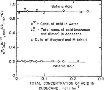
Numerous other systems have been investigated where deviations from Nernst’s distribution law can be reasonably explained by a coupling of chemical and phase-distribution equilibria. For example, data for the distribution of picric acid between water and a nonpolar solvent can be interpreted by taking into account the ionization of picric acid in the aqueous phase. In a similar manner, the distribution (i.e., the solubility) of sulfur dioxide between the gas phase and water can be described quantitatively, as shown in Chap. 10.

7.15 The Generalized van der Waals Partition Function

To calculate fluid-phase equilibria, the main requirement is a good quantitative model for representing therrnodynamic properties over a wide range of densities, from zero density (ideal gas) to close-packed density, corresponding to the compressed liquid. No currently available model is entirely satisfactory. Many of the best approximate models and theories for practical purposes are derived starting with an expression for the canonical partition function. In many cases, the simplifying concepts utilized are similar to those leading to the perturbed-hard-sphere model, first introduced by van der Waals in 1873 and cast into modern form by Zwanzig in 1954. Because so many statistical-thermodynamic models are based on the same fundamental ideas manifested in the generalized van der Waals partition function, we discuss it here in some detail.

For a binary mixture, the partition function Q depends on temperature T, total volume V, and number of molecules N₁ and N₂. The equation of state is related to Q through

(7-209)

and the chemical potentials are related to Q through

(7-210)

(7-211)

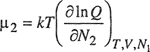
where k is Boltzmann’s constant. If Q is available as a function of T, V, N₁ and N₂, the phase-equilibrium problem is solved, at least in principle.

The partition function for a simple pure fluid containing N molecules in total volume V is (Vera and Prausnitz, 1972; Hill, 1986):

(7-212)³¹

³¹ Equation (7-212) is not truly rigorous because it assumes that contributions from repulsive forces, from attractive forces, and those from rotation, and vibration can be factored into three separate functions of temperature and density.

where A is the de Broglie wavelength³² that depends only on temperature and molecular mass; q_rep and q_att, respectively, are the contributions from repulsive and attractive intermolecular forces experienced by each molecule due to the presence of all the other molecules; and q_r,v is the contribution per molecule from rotational and vibrational degrees of freedom. For a monatomic ideal gas, the last three terms are unity. For real pure fluids, each of the last three terms depends on temperature and density.

³² A = h (2πmkT)^-l/2, where h is Planck’s constant and m is molecuiar mass.

Although van der Waals did not use partition functions, in effect, he suggested that

(7-213)

and

(7-214)

where the free volume V_f is the volume available to the center of mass of a molecule as it moves about the system, holding the positions of all other molecules fixed; E_o is the intermoiecular potential energy experienced by one molecule due to the attractive forces from all other molecules.

Equations (7-213) and (7-214), substituted in Eq. (7-212), lead to the generalized van der Waals partition function for a simple pure fluid:

(7-215)

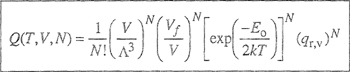
The repulsive term is determined by the free volume, V_f, and the attractive term is a Boltzmaan factor whose argument is the ratio of the attractive potential energy to the kinetic energy. For simple, small (argon-like) molecules, the final term, q_r,v, accounting for molecular rotations and vibrations is only a function of temperature but, as discussed later, for large, polyatomic molecules, q_r,v also depends on density, especially when the molecules deviate significantly from spherical shape.

To a rough first approximation, the free volume and the potential energy depend only on density; this approximation was used by van der Waals. For hard (impenetrable), spherical molecules, he assumed for V_f the simple relation (strictly valid only at low densities)

(7-216)

where V is the total volume and b = (2/3)πN_Aσ³, with molecular diameter σ and Avogadro’s constant N_A. For E_o van der Waals assumed

(7-217)

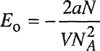
where a is a constant representing the strength of the intermolecular forces of attraction. Substituting Eqs. (7-216) and (7-217) into Eq. (7-215), assuming that q_r,v is only a function of temperature, and using Eq. (7-209) we obtain the well-known van der Waals eauation of state:

(7-218)

For large, polyatomic molecules, rotational and vibrational degrees of freedom depend on temperature and density. A small molecule (e.g., methane) can rotate and vibrate in a manner essentially independent of its environment but a large molecule (e.g., heptane) can rotate and vibrate easily only when it is remote from nearest neighbors (low density); when neighbors are close (high density), they necessarily interfere with the large molecule’s rotational and vibrational freedom. The molecule’s ability to rotate and vibrate depends on the “mean-field” exerted on it by the surrounding fluid as well as on internal modes unaffected by the surrounding fluid. For large molecules, therefore, it is not correct to assume that q_r,v [Eq. (7-215)] is only a function of temperature and independent of total volume V when the number of molecules N is fixed.

There is no accessible rigorous theory to indicate how q_r,v depends on particle density N/V and temperature. Assuming independence of external and internal contributions, q_r,v can be factored,

(7-219)

where q_ext represents contributions from external (density-dependent) rotations and vibrations while q_int represents contributions from internal rotations and vibrations; the latter contributions depend only on temperature. The external contributions may also depeed on temperature but such dependence is likely to be secondary; it is the density dependence that is of major interest.

To describe the effect of density on rotational arid vibrational contributions to the partition function, i.e. to obtain an expression for q_ext, Prigogine (1957) introduced the concept of equivalent translational degrees of freedom. The total number of external³³ degrees of freedom is the sum of the three translational degrees of freedom (possessed by every molecule, regardless of size and shape) and the equivalent translational degrees of freedom (due to rotation and vibration) that become increasingly significant as the size (and nonspfaericity) of the molecule rise. Therefore, to obtain a useful partition function, consideration must be given to the external degrees of freedom of large, polyatomic molecules.

³³ Here, “external” means influenced by density. Prigogine draws a (somewhat arbitrary) line between those degrees of freedom that are affected by density and those that are not. The latter are called internal; they depend only on temperature. External motions have relatively high amplitudes and low frequencies. Internal motions have relatively small amplitudes and high frequencies.

First, consider a large rigid molecule with r segments; all bond lengths, bond angles and torsional angles are fixed. This rigid molecule has 3 translational degrees of freedom (the same as for a spherical molecule, one for each translational coordinate) and 2 (if linear) or 3 (if not linear) rotational degrees of freedom, giving a total of 5 or 6 degrees of freedom. Second, consider a large completely flexible molecule with r segments. Here, complete flexibility means that the molecule does not have any restriction on bond length, bond angle and torsional angle. This molecule has a total maximum of 3r external degrees of freedom because in this (hypothetical) floppy molecule each segment has 3 degrees of freedom. The total number of degrees of freedom for a real large molecule lies somewhere between the limits set by a completely rigid molecule and by a completely flexible molecule. To approximate the total number of external degrees of freedom while leaving them unspecified, a parameter c is introduced. The total number of “effective” external degrees of freedom per molecule is 3c, such that 1 < c < r. For a small spherical molecule (e.g. argon or methane), r = c = 1; for more complex molecules, c > 1 (e.g. for n-decane, a possible value for c might be 2.7. For isomers of decane, c would be less than 2.7 because a branched paraffin is less flexible than a normal paraffin).

When coupled with Prigogine’s approximation that the density-dependent external rotational and vibrational degrees of freedom can be considered as equivalent translational degree of freedom, we obtain

(7-220)

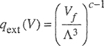
where 3(c-l) reflects the number of external rotational and vibrational motions, i.e., those rotational and vibrational motions that are affected by the presence of neighboring molecules.

Unfortunately, this expression proposed by Prigogine for q_ext does not satisfy some important boundary conditions. First, the ideal gas-limit should be obeyed, i.e. for V → ∞, (V_f/Λ³)q_ext = V/Λ³. Second, when free volume disappears as the system approaches closest-packing volume V₀, the molecules have no external degrees of freedom, i.e. for V → V₀, (V_f/Λ³)q_ext = 0.³⁴ Therefore, Beret (1975) proposed the function

³⁴ Prigogine’s original theory is restricted to liquids and liquid mixtures, including polymers, at low or moderate pressures.

(7-221)

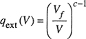
Although this expression meets all necessary boundary conditions, it was modified by Donohue (1978) to account also for the temperature dependence of q_ext:

(7-222)

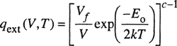
Substituting either Eq. (7-220) or Eq. (7-221) or Eq. (7-222) for q_ext into Eq. (7-215) gives a generalized van der Waals partition function for polyatomic pure fluids.

Extension of the partition function to mixtures is possible using, e.g., the fundamental idea that a mixture can be considered to be a hypothetical fluid whose characteristic properties are composition averages of the corresponding properties of the mixture’s components (one-fluid theory). Assuming that the configurational properties of a mixture are given by the one-fluid approximation, the generalized van der Waals partition function Q(T, V, N_i) for a mixture containing N₁, N₂,…, N_m molecules of components 1, 2,…, m is

(7-215a)

where N = N₁ + N₂+… + N_m is the total number of molecules in the mixture. Functions Λ_i depend only on temperature and mass m_j. However, _f, ₀, and (_r,v)_i are properties of the fluid mixture. _f and ₀ are composition averages of the corresponding pure-component properties calculated by mixing rules. For mixtures that may contain large polyatomic molecules, the procedure to account for the effect of density on rotational and vibrationa! contributions to the partition function, is the same as that for pure components. For component i in the mixture, (_r,v)_i is given by Eqs. (7-219) and (7-220) [or (7-221) or (7-222)], where V_f is now replaced by _f, e_o by ₀ and c by C_j. With these changes, substitution of either Eq. (7-220) or Eq. (7-221) or Eq. (7-222) for q_ext into Eq. (7-215a) gives a generalized van der Waals partition function for mixtures containing simple and/or polyatomic fluids.

To reduce the partition function to practice, we require expressions for free volume V_f and potential energy E_o. For mixtures we need, in addition, mixing rules (e.g. those based on the one-fluid theory) for calculating the composition-dependent properties _f and _o of the mixture. Depending on the particular expression used for q_ext and those for V_f and E_o, the generalized van der Waals partition function leads to a variety of models, e.g., the perturbed-hard-chain theory discussed in the next section and the Prigogine-Flory-Patterson theory discussed in Sec. 8.2. When c = 1, the partition function reduces to the classical van der Waals-type perturbed-hard-sphere theory.

7.16 Perturbed-Hard-Chain Theory

The serious limitations of Eq. (7-216) were known already in van der Waals’ time; attempts to improve it date back to about 1900. However, it was not until the work of Percus and Yevick (1958) and the development of molecular simulation (use of computers to simulate behavior of an assembly of molecules), that a reliable expression for V_f became available, valid at low and at high densities. This expression is (Carnahan and Starling, 1969, 1972):

(7-223)

where the reduced density η = η_cp(υ₀/υ) and .³⁵ The significance of υ₀ is that Nυ₀/N_A is the smallest possible (close-packed) volume that can be occupied by N hard spheres of diameter σ.

³⁵ The reduced density may also be written η = b/4v, the ratio (volume of molecules)/(Volume). The upper limit of v₀/v is unity. The upper limit of η is = 0.7405, the packing factor for hexagonal closest packing. Here, subscript cp stands for closest packing.

In their development of the perturbed-hard-chain (PHC) theory. Beret (1975) and Donohue (1978) used this expression to account for molecular repulsion. For q_ext they used the expression given by Eq. (7-221). For the potential energy E_o, accounting for molecular attraction, they used an analytical expression obtained from molecular-simulation studies of Alder (Alder et al, 1972) for molecules whose intermolecular forces are represented by the square-well potential:

(7-224)

Unlike the simple expression used by van der Waals [Eq. (7-217)], potential energy E_o given by Eq. (7-224) depends not only on volume but also on temperature. The 24 constants A_nm are known numbers obtained from computer-simulation data (upper limit M in the summation term depends on summation index n: n = 1, M = 6; n = 2, M = 9; n = 3, M = 5; n = 4, M = 4). Here, reduced temperature where q is the nondimensional external area of the molecule ³⁶ (q = 1 for a single arbitrarily chosen reference segment), and s is the characteristic segment-segment potential energy. Reduced volume where v^* is the characteristic hard-core volume per segment³⁷ and r is the number of segments per molecule.

³⁶ Parameter q is not to be confused with contribution q to the partition function.

³⁷ In the PHC equations, υ = V/N is the voiume per molecule. Data reduction for pure fluids gives T^*, P^* and rv^* and v^* always appear as a product.

The resulting equation of state is

(7-225)

where reduced pressure . The relationship between c and the characteristic quantities P^*, T^* and rv^* is c = P^*(rv^*)/kT^*. For each pure fluid, the PHC equation of state contains three molecular parameters εq, rv^* and c obtained from fitting experimental data, usually volumetric and vapor-pressure data.

As shown by Donohue (1978), Kaul et al. (1980) and Cotterman et al. (1986), PHC theory can be extended to mixtures using mixing rules (e.g. those based on the one-fluid theory) for calculating the composition average of the characteristic parameters , and , of the mixture. Liu (1980) showed that it can be used for mixtures of fluids with large differences in molecular size and shape (e.g., ethylene and polyethylene), and also for mixtures whose components differ appreciably in the magnitude and nature of the intermolecular forces.

To illustrate the wide range of applicability of the PHC theory, Fig. 7-29 shows a qualitative plot of molecular complexity versus density from zero density (ideal gas) to liquid-like density. The complexity scale starts with a simple molecule (argon or methane) and rises to a complex molecule, e.g., polyethylene.

Figure 7-29 Domain of perturbed-hard-chain theory, in effect, this theory interpolates with respect to molecular complexity and fluid density using known results as boundary conditions: ideaigas limit, perturbed-hard-sphere theory and Prigogine’s theory for liquid polymers.

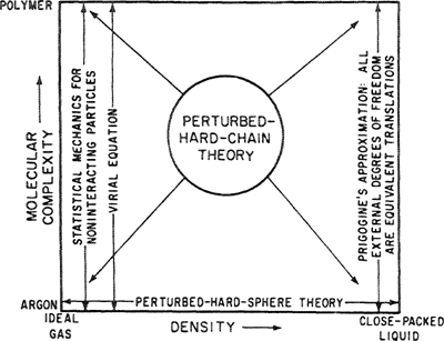
PHC theory interpolates between existing knowledge along three edges of the diagram. At low densities, PHC gives a reasonable second virial coefficient and at very low density, it reduces to the ideal-gas law. For negligible molecular complexity (c = 1), it reduces to perturbed-hard-sphere theory. For high densities. PHC is essentially identical to the Prigogine-Flory-Patterson theory of polymer liquids.

PHC theory provides a useful tool for calculating thermodynamic properties of different types of systems because it is applicable to mixtures of fluids with large differences in molecular size and shape (see Figs. 8-20 and 10-15), and also for mixtures whose components differ appreciably in the magnitude and nature of their intermolecular forces. However, because the attractive term [Eq. (7-224)] uses a fourth-order perturbation expansion, practical calculations require time-consuming computer iterations.

To simplify the equation of state and make it more useful for engineering work, several modifications have been proposed (e.g., Gmehling et al., 1979; Donohue and Vimalchand, 1988; Elliot et al., 1990; van Pelt et al, 1993). Some of these modifications are briefly discussed in Sec. 12.9 where they are used to calculate fluid-phase equilibria at high pressures.

7.17 Hard-Sphere-Chain Models

Since the early 1980’s, there has been increased interest in developing an equation of state for pure fluids and mixtures of large polyatomic molecules that does not rely on a lattice description of molecular configurations. A rigorous statistical-mechanical theory for large polyatomic molecules in continuous space is difficult because of their asymmetric structure, large number of internal degrees of freedom, and strong coupling between intra- and intermolecular interactions. Nevertheless, a relatively simple model represents chain-like molecules as freely-jointed tangent hard spheres (Dickman and Hall, 1986; Wertheim, 1987; Chapman et al., 1988; Honnell and Hall, 1989; Chiew, 1990; Mitlin and Sanchez, 1993; Thomas and Donohue, 1993; Song et al., 1994).

A hard-sphere-chain (HSC) equation of state can be used as the reference system in place of the hard-sphere reference used in most existing equations of state for simple fluids. Despite their simplicity, hard-sphere-chain models take into account some significant features of real fluids containing chain-like molecules including excluded-volume effects and chain connectivity.³⁸

³⁸ In a hard-sphere reference system, each sphere is free to move independently subject only to the restrictions of free volume. In a hard-sphere-chain reference system, each sphere (segment) is connected to at least one other sphere; therefore, the spheres (segments) cannot move independently. This lack of independence is denoted by chain connectivity.

To describe the properties of fluids consisting of large polyatomic molecules, it is necessary to introduce attractive forces by adding a perturbation to a HSC equation of state. Because the influence of attractive forces on fluid structure is weak, a van der Waals-type or other mean-field term (e.g. square-well fluids) is usually used to add attractive forces to the reference hard-sphere-chain equation of state. Although numerous details are different, most hard-sphere-chain-based equations of state follow from statistical-mechanical perturbation theory; therefore, the equation of state can be written as

(7-226)

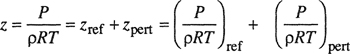
where P is pressure, ρ = N/(VN_A) is the molar density, N is the number of molecules, V is the volume of the system, and T is temperature. In Eq. (7-226), the first term represents the reference equation of state, here taken as a fluid of hard-sphere chains z_ref = z_HSC, and the second term is the perturbation to account for attractive forces.

A fortunate feature of some hard-sphere-chain-based theories is that the reference equation of state can be extended to hard-sphere-chain mixtures without using mixing rules. Only attractive terms require mixing rules.

We now summarize the reference and perturbation terms for two HSC-based equations of state.

Statistical Associated-Fluid Theory

The statistical associated-fluid theory (SAFT) (Chapman et al., 1989, 1990) is based on the first-order perturbation theory of Wertheim (1987). The essence of this theory is that the residual Helmholtz energy³⁹ is given by a sum of expressions to account not only for the effects of short-range repulsions and long-range dispersion forces but also for two other effects: chemically bonded aggregation (e.g. formation of chemically stable chains) and association and/or solvation (e.g. hydrogen bonding) between different molecules (or chains).⁴⁰

³⁹ The definition of residual Helmholtz energy is: a^R(T, V,N) = a(T,V,N)-a^id(T,V,N), where superscript id refers to an ideal gas. See App. B.

⁴⁰ The literature on SAFT is complex and confusing. The original article by Wertheira, while brilliant, is essentially incomprehensible. Much patience is required to understand what SAFT is, what it can and what it cannot do.

For a pure component, Fig. 7-30 shows a three-step process for formation of stable aggregates (e.g. chains) and subsequent association of these aggregates. Initially, a fluid consists of equal-sized, single hard spheres. In the first step, intermolecular attractive forces are added, described by an appropriate potential, such as the square-well potential (Sec. 5.5). Next, each sphere is given one, two or more “sticky spots”, such that the spheres can stick together (covalent bonding) to form dirners, trimers and higher stable aggregates such as chains. Finally, specific interaction sites are introduced at some position in the chain such that two chains can associate through some attractive interaction (e.g. hydrogen bonding.) Each step provides a contribution to the Helmholtz energy.

Figure 7-30 Three steps to form chain molecules and association complexes from hard spheres in the SAFT model.

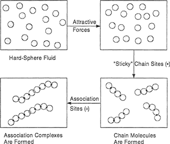
In SAFT, the residual molar Helmholtz energy a^R has contributions from formation of hard spheres and chains, from dispersion (attraction), and from association:

(7-227)⁴¹

⁴¹ A contribution a_hs is included here because of the definition of a^R given in Footnote 39.

Here the sum of the first two terms is the hard-sphere-chain reference system accounting for molecular repulsion and chain connectivity (chemical bonding); the sum of the last two terms is the perturbation accounting for molecular attraction and for association due to specific interactions like hydrogen bonding.

For a pure fluid, formation of one mole of chain molecules, each consisting of r segments, requires r moles of hard spheres. Therefore, prior to chain formation, the hard-sphere Helmholtz energy a_hs, is (Huang and Radosz, 1990)

(7-228)

where a_hs is the Helmholtz energy of one mole of the hard-sphere fluid without chain connectivity, derived by Carnahan and Starling (1969). In Eq. (7-228), r is an adjustable pure-component parameter and η, the reduced density (segment packing fraction), is

(7-229)⁴²

⁴² Equation (7-229) gives a definition of η similar but not identical to that used in Eq. (7-223).

where ρ is the molar density of chain molecules and d is the temperature-dependent effective segment diameter.⁴³ Based on the work of Barker and Henderson (1967), using a square-well potential, Chen and Kreglewski (1977) obtained

⁴³ A temperature-dependent hard-sphere diameter is to allow some overlap of spheres at high temperatures, that is, to convert hard spheres to soft spheres, for example, in the Lennard-Jones potential.

(7-230)

where σ is the temperature-independent diameter of a hard-sphere segment (it is d at T= 0 K) and ε is the temperature-independent well depth of the square potential. Because Chen and Kreglewski assumed that the ratio of the width of the square-well potential to σ is a constant, σ and ε are the only adjustable pure-component parameters with C = 0.12 for all components (Huang and Radosz, 1990). Because a characteristic volume, rather than diameter, is usually selected as a pure-component parameter (e.g., b in van der Waals-type equations of state, υ* in perturbed-hard-chain theory), a temperature-independent segment molar volume υ₀ is introduced and used as adjustable parameter:

(7-231)

where η_cp is the upper limit (closest packing) of the reduced density. υ₀ is the smallest possible (closest packed) volume that can be occupied by N_A hard-sphere segments of diameter σ.

The contribution from chain formation a_chain is (Huang and Radosz, 1990)

(7-232)

where η is the reduced density given by Eq. (7-229). Equation (7-232) follows from Wertheim’s association theory (Chapman et al., 1990), where the association bonds are replaced by covalent, chain-forming bonds.⁴⁴ It is striking that a_chain is calculated from Eq. (7-232) using three pure-component parameters r, ε and υ₀ identical to those used for calculating the hard-sphere contribution z_hs from Eq. (7-228). No additional parameter is necessary to account for chain connectivity.

⁴⁴ Chain formation is athermal; the spheres join together to form chains with no release of energy.

For the dispersion term a_disp, Huang and Radosz (1990) used an analytical expression initially obtained by Alder et al. (1972) from fitting molecular-simulation data for a square-well fluid. Alder’s expression, also the basis for the perturbed-hard-chain theory discussed in Sec. 7.16, is (per mole of chain molecules each consisting of r segments)

(7-233)

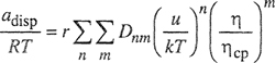
where η is the reduced density given by Eq. (7-229) with upper limit η_cp = at closest packing and u is the temperature-dependent depth of the square-well potential describing the nonspecific segment-segment interactions. As given by Chen and Kreglewski (1977), the temperature dependence of u is

(7-234)

where ε is the temperature-independent depth of the square-well potential. Constant elk in Eq. (7-234) has been related to Pitzer’s acentric factor and to critical temperature (Kreglewski, 1984) for various molecules.⁴⁵ In SAFT, the energy parameter u is for segments, not for molecules (Huang and Radosz, 1990). In Eq. (7-233), D_nm are universal constants fitted to accurate P-V-T, internal energy, and second-virial-coefficient data for argon (Chen and Kreglewski, 1977).

⁴⁵ For small molecules (e.g. argon or methane), e/k is set equal to zero. Then u is independent of temperature.

The association contribution a_assoc in Eq. (7-227) is also obtained from Wertheim’s association theory.⁴⁶ The number of association sites on a single molecule is unlimited but it must be specified. The location of the association sites, however, is not specified. The various types of sites S are labeled A, B, C,…, to keep track of the specific site-site interactions. As an example, Fig. 7-31 shows a monomer and a chain molecule, each with two different association sites, A and B. Each association site is assumed to have different interaction with the various sites on another molecule. For example, suppose A is an electron donor (Lewis base) and B is an electron acceptor (Lewis acid). In that event, we expect association whenever an A site on one molecule interacts (attraction) with a B site on another molecule. Geometric factors may hinder site-site interactions. Cluster-structure limitations, steric-hindrance approximations, and size distribution are discussed by Chapman et al. (1990).

⁴⁶ In contrast to chain formation, association of molecules (e.g. through hydrogen bonding) is not athermal. When molecules associate, energy is released.

Figure 7-31 Models for a hard-sphere (monomer) and a hard-chain molecule (r mer; a are chemical bonds), with two association sites A and B. The chain model can represent nonsphericai molecules. For example, if sites A and B attract each other, various associated complexes can be formed. This picture is not altered by converting hard spheres to soft spheres according to Eq. (7-230).

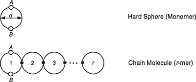
The expression for a_assoc is

(7-235)⁴⁷

⁴⁷ In Eq. (7-235), M is not to be confused with M in Eq. (7-224).

where M is the number of association sites on each molecule, X ^S is the mole fraction of molecules not bonded at specific interaction (association) site S, and the summation is over all association sites S on a molecule. X ^S is given by

(7-236)

where the summation is over all different types of sites Y = A, B, C,…; N_A is Avogadro’s constant and ρ, η and σ have the same meanings as before. The two association parameters ε^SY and K^SY characterize, respectively, the association energy and the association volume for the specific interaction between association sites S and Y. The temperature-independent segment diameter σ, used in Eq. (7-236) is related to υ₀ through Eq. (7-231).

Substitution of the expressions for ahs, a_hs, a_chain a_disp, and a_assoc in Eq. (7-227) gives the residual molar Helmholtz energy for a pure chain fluid. Application of Eq. (7-60) gives the SAFT equation of state for pure fluids. We can then write for the compressibility factor of a real fluid

(7-237)

with z^id = 1 and

(7-238)⁴⁸

⁴⁸ The hard-sphere contribution z_hs for a hard-sphere fluid without chain connectivity can also be obtained by substituting Eq. (7-223) into Eq. (7-215) with E_o = 0 (no attraction) and q_rv= 1 (no rotational and vibrational degrees of freedom) using Eq. (7-209).

(7-239)

(7-240)

(7-241)

The sum of the first three terms on the right side in Eq. (7-237) is the compressibility factor z_HSC of the hard-chain reference system accounting for molecular repulsion and chain connectivity; the sum of the last two terms is the perturbation contribution z_pert that accounts for molecular attraction and for association of different molecules (chains) due to specific interactions.

In the SAFT equation of state for pure chain fluids there are three essential adjustable parameters for nonassociating components: r, the number of segments per molecule; υ₀, the segment molar volume at closest packing; and ε, the temperature-independent depth of the square-well potential characteristic of segment-segment interactions.⁴⁹ For associating components, there are two additional parameters: the association energy ε and the association volume K^SY, characterizing the specific interaction between association sites S and Y.

⁴⁹ If the hard spheres are converted to soft spheres, there is an additional (softness) parameter C as in Eq. (7-230). If the well depth e is temperature dependent [as suggested in Eq. (7-240)], there is an additional parameter elk as in Eq. (7-234).

For mixtures, the general form of the SAFT equation of state is the same as that for pure fluids [Eq. (7-227)]. The hard-sphere contribution for mixtures is based on the theoretical result of Mansoori et al. (1971) for the equation of state for hard-sphere mixtures:

(7-242)

with

(7-243)

where p is the total molar density, x_i is the mole fraction of component i, r_i is the number of segments per molecule i, and d_i is the temperature-dependent segment diameter.

The contribution accounting for the formation of chain molecules of the various components in the mixture is

(7-244)

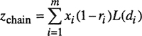
with

where ε_k (k = 2, 3) is given by Eq. (7-243). For a pure component, d_iξ₂ = ξ₃ = η given by Eq. (7-229); Eq. (7-244) then reduces to the pure-component expression given by Eq. (7-239). It is remarkable that no mixing rules are necessary in Eqs. (7-242) and (7-244). For a mixture of chain fluids, the compressibility factor of the hard-sphere-chain reference system, z_HSC = l + z_hs + z_chain can be calculated from the purecomponent parameters r_i, ε_i and v_oi. ⁵⁰ Similarly, z_assoc can be derived rigorously from statistical mechanics (Chapman et al., 1990). The relation obtained is a mole-fraction average of the corresponding pure-component equations:

⁵⁰ υ_oi gives σ_i from Eq. (7-231) and then, together with e; and parameter C, Eq. (7-230) gives dt. If the well depth ε_i, - is temperature dependent, according to Eq. (7-234) there is an additional parameter e_i/k.

(7-245)

where X^si, the mole fraction of molecules i in the mixture not bonded with other components at site S, is given by

(7-246)

with

where, as before, ξ_k(K = 2, 3) is given by Eq. (7-243) and σ_ij = (σ_i + σ_j)/2 because hard-sphere diameters are additive. In Eq. (7-246). summation is over all specific interaction sites on molecule y and summation Σ_i is over all m components.

The association/solvation parameter and the dimensionless parameter characterize, respectively, the association (i = j) and solvation (i ≠ j) energy and volume for the specific interaction between sites S and Y. These parameters are adjustable. Equation (7-246) requires no mixing rules. However, mixing rales are needed to extend Eq. (7-240) to mixtures. For mixtures, z_disp depends on the molecular size parameter r and on the segment interaction energy parameter ulkT for the mixture. Huang and Radosz (1991) proposed mixing rules for calculating the composition dependence of these parameters from the corresponding pure-component parameters. The mixing rules of Huang and Radosz are based on the van der Waals one-fluid approximation. However, for the molecular-energy parameter u, they have also proposed a volume-fraction approximation. In either case, only one adjustable binary parameter is used for the energy parameter u_ij = (u_iiu_jj,)^1/2(1–k_ij).

The SAFT equation of stale has been applied successfully to describe thermodynamic properties and phase behavior of pure fluids and fluid mixtures containing small, large, polydisperse, nonassociating and associating molecules, including super-critical and near-critical solutions of polymers (Huang and Radosz, 1990, 1991; Chen and Radosz, 1992; Gregg et al., 1993; Wu and Chen, 1994; Chen et al., 1992, 1993, 1994, 1995).

The computational requirements for SAFT applications are similar to those for other noncubic equations of state such as the perturbed-hard-chain theory. Pure component parameters for a large variety of nonassociating and associating real fluids have been tabulated (Huang and Radosz, 1990). The two different sets of mixing rules used by Huang and Radosz have been tested to correlate vapor-liquid equilibria (VLE) of fluid mixtures (Huang and Radosz, 1991). For low-pressure VLE of nonassociating and associating binary mixtures, both sets of mixing rules correlated the experimental data well. To illustrate, Fig. 7-32 shows VLE at 323 K for the mixture propanol/n-heptane. There is good agreement between experiment and SAFT calculations including the azeotrope.

Figure 7-32 Vapor-liquid equilibria at 323 K for the mixture propanol/n-heptane (Fu and Sandier, 1995).

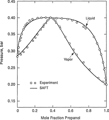
High-pressure VLE can also be correlated well with SAFT, except near the critical region. Although the volume-fraction mixing rule represents experiment near critical conditions better than the van der Waals one-fluid mixing rules, the critical region is overpredicted at high pressures and high temperatures as illustrated in Fig. 7-33 for the system CO₂/2-propanol. At 298 K, SAFT prediction agrees well with experiment including the critical region. However, at 394 K agreement is satisfactory only at low pressures.

Figure 7-33 Vapor-liquid equilibria at 298 K and 394 K for the system CO₂/2-propanol. SAFT calculations were performed with the volume-fraction mixing rule (Huang and Radosz, 1991).

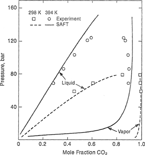
In general, SAFT correlates VLE experimental data with good accuracy, but significant deviations occur at low pressures and high temperatures, or at high pressures and low temperatures. Such deviations are not surprising because fundamentally, SAFT is a van der Waals-type theory; it has been known for many years that equations of state (or partition functions) of the van der Waals form are based on physical assumptions that are valid only at (relatively) high temperatures and high densities (Kipnis et al, 1996).

Numerous modifications have been proposed either to simplify the SAFT equation of state (e.g., Fu and Sandier, 1995; Bias and Vega, 1998) or to improve it further, e.g., for mixtures containing water (Kraska and Gubbins, 1996; Economou and Tsonopoulos, 1997). A simplified version has been developed by Galindo et al (1996, 1997), suitable for correlating high-pressure phase equilibria of aqueous mixtures. Wu (1998) has presented a SAFT-based extension of the widely used Peng-Robinson equation of state, suitable for calculating vapor-liquid equilibria of systems containing hydrocarbons, water and salt. However, the SAFT equation cannot be used for liquid-liquid equilibria in aqueous systems at normal temperatures because it cannot account for the hydrophobic effect where the dissolution of a noapolar solute (e.g. methane or ethane) causes a significant change in the molecular structure of water (see Sec. 4.10). The hydrophobic effect tends to disappear at high temperatures say, above 200°C.

The SAFT equation of state and its modifications have been successfully used to model thermodynamic properties and phase behavior for a large variety of simple and complex fluids and fluid mixtures. In Sec. 8.2 we give some examples of the application of SAFT to polymer solutions.

Perturbed Hard-Sphere-Chain Theory

The reference part of the perturbed hard-sphere-chain (PHSC) theory equation of state is based on a generalization (Song et al., 1994) of the Percus-Yevick integral-equation theory for hard-sphere chains as obtained by Chiew (1990). A simple van der Waals-type term is used for the perturbation. The PHSC equation of state for pure fluids is (Song et al, 1994)

(7-247)

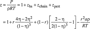
where the first three terms represent the reference equation of state for hard-sphere chains, while the last term is the van der Waals perturbation for attractive forces. Here, p is molar density. The PHSC theory does not include the effect of association.

Because parameter r and reduced density η are the same as those in the SAFT reference equation of state, contribution z_hs is also the same; however, contribution Z_chain is not. In the PHSC theory, parameter b = (2π/3)d³ is used instead of segment diameter d to calculate reduced density η defined by Eq. (7-229); η is now given by

(7-248)

In Eq. (7-247), parameter a represents the strength of attractive forces between two non-bonded segments. In PHSC theory, a and b are temperature dependent; they are given by (Song et al., 1994)

(7-249)

(7-250)

Equations (7-249) and (7-250) follow from the method of Song and Mason (1989) that scales b and a in terms of two potential parameters ε and σ; ε is the well depth of the non-bonded segment-segment pair potential and CT is the distance of separation at the minimum of the potential. In Eqs. (7-249) and (7-250), f_a and f_b, are two universal functions of a scaled temperature kT/ε. Because accurate experimental values of ε and σ exist for methane and argon, the experimental thermodynamic properties of these two fluids are used to determine the single-sphere universal functions f_a and f_b, they can be accurately represented by the following empirical formulas:⁵¹

⁵¹ A simplified version of the PHSC equation is presented here. In previous publications (e.g., Song et al., 1994), the temperature dependencies of the universal functions were scaled by a parameter j, a function of chain length r only. In the present model, this scale factor is removed and the universal functions [Eqs. (7-251) and (7-252)] were determined from the thermodynamic properties of argon and methane over a wide temperature range. Removal of s(r) from the universal functions allows use of simpler combining rules. The simpler rules do not sacrifice accuracy in fitting thermodysiamic properties of pure (non-associating) fluids to obtain equation-of-state parameters.

(7-251)

(7-252)

In the PHSC equation of state for pure fluids, there are three adjustable parameters: r, σ, and ε. Song et al. (1994a) have applied the PHSC equation of state to describe theraiodynamic properties of normal fluids and polymers and made parameters available for a wide variety of polymers and normal fluids.

The PHSC equation of state is extended to mixtures according to

(7-253)

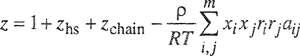
where Z_hs of the hard-sphere mixture is the same as that in the SAFT equation of state, given by Eqs. (7-242) and (7-243) with d_i³ = (3/2π)b_i. In Eq. (7-253), z_chain, the contribution accounting for the formation of chain molecules, is

(7-254)

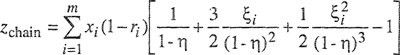
where the reduced density of hard-sphere mixtures is given by

(7-255)

and

(7-256)

For one-component systems and for mixtures of equal-sized spheres, ε_i = η.

As in Eq. (7-247), the first three terms in Eq. (7-253) represent the reference equation of state for hard-sphere-chain mixtures and the last term is a van der Waals-type perturbation for attractive forces. Like in the SAFT equation of state, for a mixture of chain fluids, the compressibility factor of the hard-sphere-chain reference system, z_HSC = 1 + z_hs+z_chain can be calculated from pure-component parameters r_i, ε_i and b_i only.

However, for each unlike pair of components (i ≠ j), an additional parameter a_ij is needed for the mixture. Its physical meanings is similar to that for pure fluids: a_ij reflects the strength of attractive forces between two nonbonded segments i and j. An expression for a_ij is obtained by extending Eq. (7-249) to mixtures:

(7-257)

where σ_ij is given by σ_ij = (σ_i + σ_j)/2 and ε_ij is related to the pair potential between unlike segments, given by

(7-258)

Therefore, only one binary adjustable parameter k_ij is required.

Although the PHSC equation of state can be used to model thermodynamic properties and phase behavior of normal fluids, polymers and their mixtures, it has been primarily applied to polymer mixtures. Song et al. (1994a) found that, for nonassociated mixtures, the PHSC equation of state performs as well as the SAFT equation of state, as expected, because these two models share many basic ideas. Section 8.3 presents examples that illustrate the application of the PHSC equation of state to polymer mixtures.

A second-order perturbation theory based on the hard-sphere-chain reference system is given by Hino (1997). Because of the second-order correction, it is better than Song’s theory at low temperatures. Also, because Hino’s results, based on the work of Chang and Sandier (1994), use a square-well potential of variable width, Hino’s work is applicable to a wider variety of mixtures.

7.18 Summary

The theory of solutions is an old subject. Many of the articles in the first volumes of the Zeitschrift fur Physikalische Chemie (around 1890) are concerned with the properties of liquid mixtures; since the early days of physical chemistry, thousands of articles have been written in an effort to understand the behavior of mixed fluids. While much progress has been made, we are still far from an adequate theory of liquid mixtures. In this chapter we have indicated a few of the theoretical ideas that have been proposed and it is evident that none of them is sufficiently broad to apply to the general problem; rather, each idea and each model appears to be limited to a particular class of solutions. As a result, while we do not have a general theory of liquid mixtures, we have instead, a variety of restricted theories and models, each useful for a particular type of mixture.

To construct a theory of liquid mixtures, we require essentially two kinds of information: We need to know something about the structure of liquids (i.e., the way the molecules in a liquid are arranged in space), and we need to know something about intermolecular forces between like and unlike molecules. Unfortunately, information of either kind is inadequate and, as a result, all of our theories must make simplifying assumptions to overcome this disadvantage. Because simplifying assumptions must be made, it follows that we cannot at this time construct a general theory; simplifying assumptions that are reasonable for one type of mixture (e.g., mixtures of hydrocarbons) may be most unreasonable for another (e.g., aqueous mixtures of organic acids) and, because the simplifying assumptions must vary from one type of mixture to another, we inevitably have different theories and models for different applications: The punishment must fit the crime.

Most theoretical work has been concerned with mixtures of liquids whose molecules are nonpolar and spherical. Some of this work has been indicated here: Regular-solution theory, lattice theory and perturbation theory, all start out with simple molecules and are then extended, often semiempirically, to more complicated molecules. Recent theoretical work on mixtures of simple molecules (theories based on the radial distribution function) has not been discussed in detail because an adequate treatment requires more familiarity with statistical mechanics than we can give here. Some of these theories promise to contribute to our understanding of liquid structure, but they do not tell us anything about intermolecular forces between dissimilar molecules. To use these theories, we mast include independent information on intermolecular forces.

For mixtures of nonpolar liquids, the regular-solution theory of Scatchard and Hildebrand frequently provides a good approximation for the excess Gibbs energy. The most serious simplifying assumption in this theory is the geometric-mean rule for the cohesive energy density of the unlike (1-2) interaction. For application, whenever possible, this geometric-mean rule should be modified empirically by utilizing whatever limited experimental binary data may be available. Two important advantages of the Scatchard-Hildebrand regular-solution theory are its simplicity and its ease of extension to systems containing more than two components.

Regular-solution theory, like most theories of solution, is more reliable for excess Gibbs energy than for excess enthalpy and excess entropy. All simple theories of solution neglect changes in molecular vibration and rotation that result from the change of molecular environment that is inevitably produced by mixing; these changes, in some cases, affect the excess enthalpy and excess entropy in such a way that they tend to cancel in the excess Gibbs energy, at least to a first approximation.

The lattice theory of solutions, although first developed for monatomic molecules, can be extended to molecules of more complex structure using well-defined assumptions, as shown by Guggenheim, Flory, and others. This extension makes it particularly useful for solutions of molecules that differ appreciably in size, such as polymer solutions, as discussed in Chap. 8. However, the concept of a lattice for liquid structure is a vast oversimplification; and as a result, lattice theory becomes increasingly inappropriate as attention is focused on temperatures remote from the melting point. Also, for each binary system, lattice theory requires as an input parameter the interchange energy w (or its equivalent, the Flory parameter x), that is difficult to predict and that, unfortunately, is temperature-dependent. Because the lattice concept is not truly appropriate for liquids, reduction of experimental data for real mixtures often gives an exchange energy that depends also on composition. In that event, lattice theory requires extensive empirical modifications.

Most simple theories of mixtures assume random mixing of molecules; for strongly nonideal mixtures, this assumption can lead to serious error. Although we do not have a rigorous theory of nonrandom mixtures, a fair description is sometimes obtained by using the quasi-chemical approximation. A semiempirical generalization of that approximation is provided by the concept of local concentration leading to the equations of Wilson, NRTL, and UNIQUAC. These equations do not have a precise theoretical basis but appear to be of a form that is particularly useful for solutions containing one or more polar components.

For those who favor a philosophy of idealism, it is attractive to do away with nonideality in solutions by claiming that our observations of nonideality are merely apparent, that all solutions are, in fact, ideal if only we use in our calculations the true, rather than the apparent, molecular concentrations. This idealistic view attributes all observed nonideality to formation of new chemical species in solution; by postulating association or solvation equilibria (or both) and then letting equilibrium constants be adjustable parameters, one can indeed fit experimental data for many liquid mixtures. The chemical theory of solutions permits us to fit experimental data for any liquid mixture, regardless of complexity, provided that we use a sufficient number of adjustable equilibrium and stoichiometric constants.

The chemical theory of solutions provides a sensible approximation whenever there is independent evidence that strong chemical forces operate in the liquid mixture; for example, whenever there is appreciable hydrogen bonding between like or unlike components (or both), it is reasonable to assume that the formation (or dissociation) of hydrogen-bonded molecules in solution provides the dominant contribution to the solution’s thermodynamic properties. If chemical forces are strong, then physical (vander Waals) forces may often be neglected, at least for a first approximation, but careful study has shown that for accurate work both physical and chemical forces must be taken into account. However, the dividing line between physical and chemical forces cannot easily be determined with rigor and as a result, it is often necessary to make an essentially arbitrary decision on where that line is drawn.

The vagueness of the chemical theory of solutions provides a wide range of possible applications. However, we must beware of the strong temptation to use it where, because of other physical evidence, it is inapplicable. Any theory of solutions with a sufficient number of adjustable parameters must always be viewed with suspicion unless supported by independent physicochemical measurements. Nevertheless, when used judiciously, the chemical theory of solutions provides a useful framework for correlating and extending thermodynamic data for strongly nonideal solutions where currently available physical theories are inappropriate.⁵²

⁵² A major deficiency of the Dolezalek chemical theory follows from its inability to account for phase separation (demixsng). This deficiency, however, is removed by the extensions given in Sees. 7.11 and 7.12.

Reasonable (but nevertheless approximate) theories are now available for mixtures that contain chain-like molecules in addition to “normal”, essentially spherical (or globular) molecules. These theories (perturbed hard chain, statistical associated fluid, perturbed hard chain of spheres) have a wider range of applicability than those based on a (hole-free) lattice because they are based on equations of state that (unlike a hole-free lattice) give the segment density as a function of temperature, pressure and composition. Further, these equation-of-state theories can incorporate association between like molecules and solvation between unlike molecules. Regrettably, even for nonpolar fluids, these equations-of-state theories require several (typically 3 or 4) pure-component molecular parameters; if the molecules associate, additional pure-component parameters are needed. For simple cases (e.g. mixtures of hydrocarbons), one binary parameter may be sufficient but often two are needed; for solutions where solvation is important, additional binary parameters must be specified. The need for so many parameters follows from our inadequate understanding of intermolecular forces.

Ever-increasing impressive advances in molecular simulation are likely to exert a dramatic influence on our future ability to describe the properties of liquid mixtures. Such simulations not only serve to test the physical significance of analytic models but also to suggest new and improved models. Some day, when computers become even more powerful than they are now, it may be possible to calculate thermodynamic properties of liquid mixtures on a routine basis without any need for equations of state or other analytical models. But as of now (1998), that day is still far in the future.

In general, we may say that theories of solutions are mental crutches that enable us to order, interpret and in a vague sense “understand” thermodynamic data for mixtures. These theories provide a framework that enables us to correlate data in a sensible manner; they tell us what to plot against what, the coordinates we must use to obtain a smooth (and perhaps evea straight) line. For engineering work, such a framework is extremely useful because it enables us to interpolate and extrapolate limited experimental results and to make reasonable predictions for systems not previously studied, especially for those systems containing more than two components. Finally, however, it is important to remember, as Scatchard has pointed out, ⁵³ that theories of solution are, essentially, working tools; we must not take any theory too seriously because real liquid mixtures are much more complicated than our oversimplified models.

⁵³ “The best advice that comes from years of study of liquid mixtures is to use any model insofar as it helps, but not to believe that any moderately simple model corresponds very closely to any real mixture” (1949, Chem, Rev., 44: 7), This advice is a specific example of what A. N. Whitehead has called “the fallacy of misplaced concreteness,” i.e., the tempting but erroneous habit of theorists to regard theoretical models as reality, rather than idealized representations of reality.

To make progress, we must keep in mind the simplifying assumptions on which our theories are based, for, as Francis Bacon said many years ago, “Truth is more likely to emerge from error than from confusion.”

References

Abrams, D. S. and J. M. Prausnitz, 1975, AIChE J., 21: 16.

Alder, B. J., D. A. Young, and M. A. Mark, 1972, J. Chem. Phys., 56: 3013.

Aveyard, R. and R. W. Mitchell, 1970, Trans. Faraday Soc., 66: 37.

Barker, J. A., 1963, Lattice Theories of the Liquid State. Oxford: Pergamon Press.

Barker, J. A. and D. Henderson, 1967, J. Chem. Phys., 47: 4714.

Barton, A. F. M., 1991, Handbook of Solubility Parameters. Boca Raton: CRC Press.

Bazúa, E. R. and J. M. Prausnitz, 1971, Cryogenics, 11: 114.

Beret, S. and J. M. Prausnitz, 1975, AIChE J., 21: 1123.

Blanks, R. F. and J. M. Prausnitz, 1964, Ind. Eng. Chem. Fundam., 3: 1.

Bias, F. J. and L. F. Vega, 1998, Ind. Eng. Chem. Res., 37: 660.

Burrell, H., 1955, Interchem. Rev., 34: 3, 31. Burrell, H., 1968, J. Paint Technol, 40: 197.

Burrell, H., 1975, Solubility Parameter Values. In Polymer Handbook, 2¡^d Ed. (J. Brandrup, and E. H. Immergut, Eds.). New York: John Wiley & Sons.

Carnahan, N. F. and G. J. Yevick, 1958, Phys. Rev., 110: 1.

Carnahan, N. F. and K. E. Starling, !912, AIChE J., 18: 1184.

Chang, J. and S. I. Sandier, 1994, Mol. Phys., 81: 735, 745. Chao, K. C. and G. D. Seader, 1961, AIChE J., 7: 598.

Chapman, W. G., G. Jackson, and K. E. Gubbins, 1988, Molec. Phys., 65: 1057.

Chapman, W. G., K. E. Gubbins, G. Jackson, and M. Radosz, 1989, Fluid Phase Equilibria, 52: 31.

Chapman, W. G., K. E. Gubbins, G. Jackson, and M. Radosz, 1990, Ind. Eng. Chem. Res., 29: 1709.

Chen, S. S. and A. Kreglewski, 1977, Ber. Bunsenges. Phys. Chem., 81: 1048.

Chen, S.-J. and M. Radosz, 1992, Macromolecules, 25: 3089.

Chen, S.-J., I. G. Economou, and M. Radosz, 1992, Macromolecules, 25: 4987.

Chen, S.-J., I. G. Economou, and M. Radosz, 1993, Fluid Phase Equilibria, 83: 391.

Chen, S.-J., Y. C. Chiew, J. A. Gardecki, S. Nilsen, and M. Radosz, !994, J. Polym. Sci, Part B: Polym. Phys., 32: 1791.

Chen, S.-J., M. Banaszak, and M. Radosz, 1995, Macromolecules, 28: S812.

Cheung, H. and E. H. Zander, 1968, Chem. Eng. Prog. Symp. Ser., 64: 34.

Chiew, Y. C., 1990, Molec. Phys., 70: 129.

Cotterman, R. L., B. J. Sehwarz, and J. M. Prausnitz, 1986, AIChE J., 32: 1787.

Croll, I. M. and R. L. Scott, 1958,/. Phys. Chem., 62: 954.

Derr, E. L. and C. H. Deal, 3969, Inst. Chem. Eng. Symp. Ser., (London), 3: 40.

Derr, E. L. and C. H. Deal, 1973, Adv. Chem. Ser., 124: 11.

Dickman, R. and C. K. Hall, J. Chem. Phys., 1986, 85: 4108.

Dolezalek, R, 1908, Z. Phys. Chem., 64: 727.

Donohue, M. D. and J. M. Prausnitz, 1975, Can. J. Chem., 53: 1586.

Donohue, M. D. and J. M Prausnitz, 1978, AIChE J., 24: 849.

Eckert, C. A., 1964, Dissertation, University of California, Berkeley.

Economou, I. G. and C. Tsonopoulos, 1997, Chem. Eng. Sci., 52: 511.

Ellis, J. A. and K.-C. Chao, 1972, AIChE J., 18: 70.

Fast, J. D., 1962, Entropy, Philips Technical Library. Eindhoven, The Netherlands: Centrex Publishing Co.

Fisher, G. D. andT. W. Leland, 1970, Ind. Eng. Chem. Fundam., 9: 537.

Flory, P. J., 1941, J. Chem. Phys., 9: 660.

Flory, P. J., 1942, J. Chem. Phys., 10:51.

Flory, P. J., 1944, J. Chem. Phys., 12: 425.

Flory, P. J., 1953, Principles of Polymer Chemistry. Ithaca: Cornell University Press.

Fredensiund, Aa., R. L. Jones, and J. M. Prausnitz, 1975, AIChE I, 2: 1086.

Fredensiund, Aa., J. Gmehling, M. L. Michelsen, P. Rasmussen, and I. M. Prausnitz, 1977, Ind. Eng. Chem. Process Des. Dev., 16: 450.

Fredensiund, Aa., G. Gmehling, and P. Rasmussen, 3977a, Vapor-Liquid Equilibria Using UNIFAC. Amsterdam: Elsevier⁵⁴.

⁵⁴ The latest compilation of UNIFAC parameters (with pertinent computer programs) is available from J. M. Prausnitz, Department of Chemical Engineering, University of California, Berkeley, CA 94720, USA.

Fredensiund, A. and P. Rasmussen, 1985, Fluid Phase Equilibria, 24:115.

Fredensiund, Aa. and J. M. Sørensen, 1994, Group-Contribution Estimation Methods. In Models for Thermodynamic and Phase-Equilibria Calculations, (S. I. Sandier, Ed.). New York: Marcel Dekker.

Fu, Y. H. and S. I. Sandier, 1995, Ind. Eng. Chem. Res., 34: 1897.

Funk, E. W. and J. M. Prausnitz, 1970, Ind. Eng. Chem., 62: 8.

Galindo, A., P. J. Whitehead, G. Jackson, and A. N. Burgess, 1996, J. Phys. Chetn., 100: 6781.

Galindo, A., P. J. Whitehead, G. Jackson, and A. N. Burgess, 1997, J. Phys. Chem. B, 101: 2086.

Gamson, B. W. and K. M. Watson, 1944, Natl. Petrol. News, R623 (August 2; Sept. 6).

Gardon, J. L., 1966, J. Paint Technol, 38: 43.

Gmehling, J., D. D. Liu, and J. M. Prausnitz, 1979, Chem. Eng. Sci, 34: 951.

Gmehling, J., 1986, Fluid Phase Equilibria, 30: 119.

Gmehling, J., J. Li, and M. Schiller, 1993, Ind. Eng. Chem. Res., 32: 178.

Gonsalves, J. B. and T. W. Leland, 1978, AIChE J., 24: 279.

González, J. A., I. Garcia de la Fuente, and J. C. Cobos, 1997, Fluid Phase Equilibria, 135: 1.

González, J. A., I. Garcia de la Fuente, and J. C. Cobos, 1997a, J. Chem. Soc. Faraday Trans., 93:3773.

Gregg, C. J., S.-J. Chen, F. P. Stein, and M. Radosz, 1993, Fluid Phase Equilibria, 83: 375.

Guggenheim, E. A., 1952, Mixtures. Oxford: Oxford University Press.

Guggenheim, E. A., 1966, Applications of Statistical Mechanics. Oxford: Oxford University Press.

Gunning, A. J. and J. S. Rowlinson, 1973, Chem. Eng. ScL, 28: 521.

Gupte, P. A. and R. P. Banner, 1987, Ind. Eng. Chem. Res., 26: 2036.

Hansen, C. M., 1967, J. Paint Technol, 39: 104, 505.

Hansen, C. M. and K. Skaarap, 1967,/. Paint Technol., 39: 511.

Hansen, C. M. and A. Beerbower, 1971, Solubility Parameters. In Encyclopedia of Chemical Technology (Kirk-Othmer), 2^nd; Ed., Suppl. Vol. (H. F. Mark, J. J. McKetta, and D. F. Othmer Eds.). New York: Wiley-Interscience. See also Barton, 1991.

Hansen, H. K., P. Rasmussen, Aa. Fredenslund, M. Schiller, and J. Gmehling, 1991, Ind. Eng. Chem. Res., 30: 2352.

Harris, H. G. and J. M. Prausnitz, 1969, Ind. Eng. Chem. Fundam., Wilhelm Memorial Issue (May).

Heil, J. F. and J. M. Prausnitz, 1966, AIChE J., 12: 678.

Heintz, A., 1985, Ber. Bunsenges. Phys. Chem., 89: 172.

Heintz, A. and D. Papaioannou, 1998, Thennochimica Acta, 310: 69.

Henderson, D. and P. J. Leonard, 1971. In Physical Chemistry, Vol. VIIIB: Liquid State (D. Henderson, Ed.), Chap. 7. New York: Academic Press.

Hicks, C. P., 1972,/Chem. Soc. Faraday Trans II, 72: 423.

Hildebrand, 1929, J. H.,/. Am. Chem. Soc., 51: 66.

Hildebrand, J. H., 1947,/. Chem. Phys., 15: 225.

Hildebrand, J. H. and R. L. Scott, 1950, The Solubility of Nonelectrolytes, 3^nd Ed. New York: Rein-hold.

Hill, T. L., 1986, An Introduction to Statistical Thermodynamics. Reading: Addition-Wesley.

Hino, T. and J. M. Prausnitz, 1997, Fluid Phase Equilibria, 138: 105.

Honnell, K. G. and C. K. Hal!, 1989, J. Chem. Phys., 90: 1841.

Hooper, H. H., S. Michel, and J. M. Prausnitz, 1988, Ind. Eng. Chem. Res., 27: 2182.

Hovorka, F. and D. Dreisbach, 1934, J. Am. Chem. Soc., 56: 1664.

Huang, S. H. and M. Radosz, 1990, Ind. Eng. Chem. Res., 29: 2284.

Huang, S. H. and M. Radosz, 1991, Ind. Eng. Chem. Res., 30: 1994.

Huggins, M. L., 1941,/Phys. Chan., 9: 440.

Huggins, M. L., 1942, Ann. N. Y. Acad. ScL, 43: 1.

Joffe, J., 1948, Ind. Eng. Chem., 40: 1738.

Johnson, A. I., W. F. Furter, and T. W. Barry, 1954, Can. J. TechnoL, 32: 179.

Kammerer, K., S. Schnabel, D. Silkenbaumer, and R. N. Lichtenthaler, 1999, Fluid Phase Equilibria, 162: 289.

Kaul, B. K., M. D. Donohue, and J. M. Prausnitz, 1980, Fluid Phase Equilibria, 4: 171.

Kay, W. B., 1936, Ind. Eng. Chem., 28: 1014.

Kehiaian, H. V., 1983, Fluid Phase Equilibria, 13: 243.

Kehiaian, H. V., 1985, Pure & Appl. Chan., 57: 15.

Kipnis, A. Ya., B. E. Yavelov, and J. S. Rowlinson, 1996, Van der Waals and Molecular Science. Oxford: Clarendon Press.

Kohler, F., 1957, Monatsh. Chem., 88: 857.

Kortüm, G. and H. Buchhoiz-Meisenheimer, 1952, Die Theorie der Destination und Extraktion von Flussigkeiten, Chap. 3. Berlin: Springer. See also the reference in Footnote 22.

Krasha, T. and K. E. Gubbins, !996, Ind. Eng. Chem. Res., 35: 4727, 4738.

Kreglewski, A.. 1984, Equilibrium Properties of Fluids and Fluid Mixtures. Coliege Station: Texas A&M University Press.

Kretschmer, C. B. and R. Wiebe, 1954, J. Chem. Phys., 22: 1697.

Larsen, B. L., P. Rasmussen, and A. Fredensiund, 1987, Ind. Eng. Chem. Res., 26: 2774.

Leach, J. W., P. S. Chappelear, and T. W. Leland, ! 968, AlChE J., 14: 568.

Lee, B. I. and M. G. Kesler, 1975, AIChE J., 21: 510.

Leland, T. W., P. S. Chappelear, and B. W. Gamson, 1962, AIChE J., 8: 482.

Leland, T. W., J. S. Rowlinson, and G. A. Sather, 1.968, Trans. Faraday Soc., 64: 1447.

Leland, T. W., J. S. Rowlinson, G. A. Sather, and I. D. Watson, 1969, Trans. Faraday Soc., 65: 2034.

Lichtenthaler, R. N., D. S. Abrarns, and J. M. Prausnitz, 1973, Can. J. Chem., 51: 3071.

Lichtenthaler, R. N., D. D. Liu, and J. M. Prausnitz, 1974, Ber. Bunsenges. Phys. Chem., 78: 470.

Liu, D. D. and J. M. Prausnitz, 1980, Ind. Eng. Chem. Process Des. Dev., 19: 205.

Macedo, E. A., U. Weidlich, J. Gmehling and P. Rasmussen, 1983, Ind. Eng. Chem. Process Des. Dev., 22: 676.

Magnussen, T., P. Rasmussen, and A. Fredensiund, 1981, Ind. Eng. Chem. Res., 20: 331.

Mansoori, G. A., N. F. Carnahan, K. E. Starling, and T. W. Leland, 1971, J. Chem. Phys., 54: 1523.

Mark, H. F., J. J. McKetta, and D. F. Othmer, 1969, (Eds.), Encyclopedia of Chemical Technology (Kirk-Othmer), 2^nd Ed., Vol. 18, pp. 564-588. New York: Wiley-lnterscience.

Marsh, K. N., 1980, Ann. Rep. Prog. Chemistry, Sec. C, R. Soc. Chem. (Land.), 77: 101.

Martin. R. A. and K. L. Hoy, S975, Tables of Solubility Parameters. Tarrytown: Union Carbide Corp., Chemicals and Plastics, Research and Development Dept. (See also Moelwyn-Hughes, 1940).

Maurer. G. and J. M. Prausnitz, 1978, Fluid Phase Equilibria, 2:91.

McGJashan, M. L. and R. P. Rastogi, 1958, Trans. Faraday Soc., 54: 496.

McGIashan, M. L., 1962, Chem. Soc. (Land.), Annu. Rep., 59: 73.

Mecke, R., 1948, Z. Eiektrochem., 52: 274.

Mitlin, V. S. and I. C. Sanchez, 1993,/. Chem. Phys., 99: 533.

Moelwyn-Hughes, E. A., 1940, J. Chem. Soc., 850.

Nagata, 1, 1977, Fluid Phase Equilibria, 1: 93.

Nagata, L, 1978, Z. Phys. Chem. Lelpzig, 259: 1109, 1151.

Nagata, I, K. Tamura, N. Kishi, and K. Tada, 1997, Fluid Phase Equilibria, 135: 227.

Nelson, R. C., R. W. Hemwall, and G. D. Edwards, 1970, J. Paint TechnoL, 42: 636.

Nernst, W., 1891, Z. Phys. Chem., 8: 110.

Null, H. R. and D. A. Palmer, 1969, Chem. Eng. Prog., 65: 47.

Null, H. R., 1970, Phase Equilibrium in Process Design. New York: John Wiley & Sons.

Ormanoudis, C. and C. Panayiotou, 1993, Fluid Phase Equilibria, 89: 217.

Orye, R. V. and J. M. Prausnitz, 1965, Ind. Eng. Chem., 57: 18.

Panayiotou, C., 1988, J. Phys. Chem., 92: 2960.

Panayiotou, C. and I. C. Sanchez, 1991, J. Phys. Chem., 95: 10090.

Panayiotou, C., 1997, Fluid Phase Equilibria, 131: 21.

Pimentel, G. and A. L. McClellan, 1960, The Hydrogen Bond. San Francisco: Freeman.

Plöcker, U., H. Knapp, and J. M. Prausnitz, 1978, Ind. Eng. Chem. Process Des. Dev., 17: 324.

Preston, G. T. and J. M. Prausnitz, 1970, Ind. Eng. Chem. Process Des. Dev., 9: 264.

Prigogine, I., V. Mathot, and A. Desmyter, 1949, Bull Soc. Chim. Belg., 58: 547.

Prigogine, I. and A. Desmyter, 1951, Trans. Faraday Soc., 47: 1137.

Prigogine, I. and R. Defay, 1954, Chemical Thermodynamics, Chap. 26. London: Longmans & Green.

Prigogine, L, 1957, The Molecular Theory of Solutions. Amsterdam: North-Holland.

Redlich, O. and A. T. Kister, 1947, J. Chem. Phys., 15: 849.

Renon, H. and J, M. Prausnitz, 1967, Chem. Eng. Sci, 22: 299.

Errata, 1891. Renon, H. and J. M. Prausnitz, l969, AIChEJ., 15: 785.

Scatchard, G., 1949, Chem. Rev., 44: 7.

Scott, R. L., 1956, Annu. Rev. Phys. Chem., 1: 43. Scott, R. L., 1956a, J. Chem. Phys., 25: 193.

Scott, R. L., 1958, J. Phys. Chem., 62: 136.

Skjold-Jørgensen, S., B. Kolbe, J. Gmehling, and P. Rasmussen, 1979, Ind. Eng. Chem. Process Des. Dev., 18: 714.

Smith, F. and I. Brown, 1973, Aust. J. Chem., 26: 691, 705. Smith, W. R., 1972, Can. J. Chem. Eng., 50: 271.

Song, Y. and E. A. Mason, 1989, J. Chem. Phys., 91: 7840.

Song, Y., S. M. Lambert, and J. M. Prausnitz, 1994, Macromolecules, 27: 441.

Song, Y., S. M. Lambert, and J. M. Prausnitz, 1994a, Ind. Eng. Chem. Res., 33: 1047.

Staverman, A. J., 1950, Reel. Trav. Chim. Pays-Bas, 69: 163.

Thomas, A. and M. D. Donohue, 1993, Ind. Eng. Chem. Res., 32: 2093.

Thorp, N. and R. L. Scott, 1956, J. Phys. Chem., 60: 670, 1441.

Tompa, H., 1952, Trans. Farad. Soc., 48: 363.

Tucker, E. E. and E. Lippert, 1976. In The Hydrogen Bond: Recent Developments in Theory and Experiment (P. Schuster, G. Zundel, and C. Sandorfy, Eds.), Chap. 17. Amsterdam: North-Holland.

Tucker, E. E. and S. D. Christian, 1978, J. Phys. Chem., 82: 1897.

Van Laar, J. J., 1910, Z. Phys. Chem., 72: 723.

Van Ness, H. C., J. van Winkle, H. H. Richtol, and H. B. Hollinger, 1967, J. Phys. Chem., 71: 1483.

Van Pelt, A., C. J. Peters, and J. de Swaan Arons, 1993, Fluid Phase Equilibria, 84: 23.

Vera, J. H. and J. M. Prausnitz, 1972, Chem. Eng. J., 3: 1.

Waish, J. M. and K. E. Gubbins, 1990, J. Chem. Phys., 94: 5115.

Watson, I. D. and J. S. Rowlinson, 1969, Chem. Eng. ScL, 24: 1575.

Weimer, R. F. and J. M. Prausnitz, 1965, Hydrocarbon Process. Petrol. Refiner., 44: 237. Wertheim, M. S., J. Chem. Phys., 1987, 87: 7323.

Wilson, G. M., 1964, J. Am. Chem. Soc., 86: 127.

Wu, C.-S. and Y.-P. Chen, 1994, Fluid Phase Equilibria, 100: 103.

Wu, J. and J. M. Prausnitz, 1998, Ind. Eng. Chem. Res., 37: 1634.

Problems

1. A liquid hydrocarbon A has a saturation pressure of 13.3 kPa at 10°C. Its density at 25°C is 0.80 g cm"³ and its molecular weight is 160. This is ail the information available on pure liquid A. An equimolar mixture of A in carbon disulfide at 10°C gives an equilibrium partial pressure of A equal to 8 kPa. Estimate the composition of the vapor that at 10°C is in equilibrium with an equimolar liquid solution of A in toluene, using the follow data

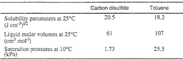
2. Consider a dilute isothermal solution of acetic acid in benzene. For the dilute region (say up to 5 mol % acid), draw schematically curves for versus x₁ and versus x₁ where subscript 1 refers to the acid. Briefly justify your schematic graphs with suitable explanations.

3. For distillation-column design, we need K factors (K_i = y_i/x_i). A liquid mixture at 50°C contains 30 mol % n-hexane and 70 mol % benzene. Calculate the K factors of n-hexane and benzene in this mixture. Assume that the pressure is sufficiently low to neglect gas-phase corrections and Poynting factors. At 50°C, pure-component vapor pressures are 0.533 bar for n-hexane and 0.380 bar for benzene.
At 25°C, the molar volumes and solubility parameters are:

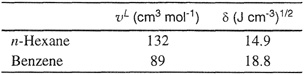
4. Consider a solution of diethyl ether and pentachloroethane. Draw (schematically) a plot of g^E versus x at constant temperature. Briefly justify your schematic graph with suitable explanations.

5. Liquids A and B when mixed form an azeotrope at 300 K and at a mole fraction x_A = 0.5. It is desired to separate a mixture of A and B by distillation, and in order to break the azeotrope it is proposed to add a third liquid C into the mixture. Compute the relative volatility of A to B at 300 K when the ternary mixture contains 60 mol % C and equal molar amounts of A and B. Assume ideal gas behavior and assume that A, B, and C are nonreactive nonpolar substances. The data given below are all at 300 K.

6. A binary liquid mixture contains nonpolar components 1 and 2. The mixture is to be separated by ordinary distillation. To determine if this is feasible, it is necessary to know whether the mixture has an azeotrope. At 300 K the pure-component vapor pressures are = 53.3 and = 80 kPa. The pure-component molar volumes are both 160 cm³ mol¹ and the solubility parameters are δ₁= 14.3 and δ₂= 17.4 (J cm^-3)^1/2. At 300 K, does this mixture have an azeotrope? If so, what is its composition? Assume the vapor phase is ideal.

7. At 380 K, an equimolar liquid mixture of A and B has a total pressure of 0.667 bar. Fluids A and B are simple nonpolar liquids having similar molar volumes. Pure-component vapor pressures (bar) are = 0.427 and = 04.93
If the equimolar mixture is cooled, partial miscibility (two liquid phases) results. Give an estimate of the (upper) critical solution temperature where partial miscibility begins. Explain and justify your method of calculation. Is your estimate likely to be high or low? Give an upper and lower bound of the expected (upper) critical solution temperature.

8. An equimolar liquid mixture of benzene and n-butane is fed to an isothermal flash tank operating at 50°c and 1 bar.

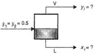
Find the compositions of the two streams leaving the flash tank.assume that at 1 bar the gas is ideal. assume also that for the liquid phase, the Scatchard-Hildebrand (regular-solution) equations are valid.
Data (all at 50°C)are as follows:

9. Estimate the upper critical solution temperature for a binary system containing nonpolar liquids A and B.
Data at 25°C:

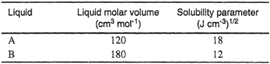
10. At 25°C, carbon disulfide (1)and perfluoro-n-heptane (2) are essentially totally immiscible. A small amount of cyclohexane (3) is added to this two-phase mixture. Estimate the distribution coefficient k for cyclohexane[k = x₃(in 1)/x₃(in 2)].
Pure component data:

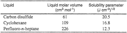
11. Chemical engineers are fond of generalized plots. Show how you would prepare a generalized solubility parameter plot for nonpolar liquids based on pitzer’ s three-parameter theory of corresponding states.

12. At room temperature and atmospheric pressure:

(a) Give an order-of-magnitude estimate of for methanol dissolved in a large excess of isooctane.

(b) Give an order-of-magnitude estimate of the change in temperature when equal parts of cyclohexane and carbon disulfide are mixed adiabatically. Is ΔT positive or negative?

(c) Name two polar solvents that are likely to be very good and two others that are likely to be very poor for an extraction separation of hexane and hexene. Explain.

13. A dilute solution of picric acid in water is contacted with n-hexane. Consider the distribution of picric acid between the two solvents; assume that the acid exists as a monomer in both phases but that it ionizes partially in the aqueous phase. Show that the distribution of the acid should be described by an equation of the form

where c_H is the concentration of picric acid in hexane, c_w is the concentration of picric acid in water, and a and b are constants depending only on temperature.

14. Acetaldehyde forms a trimer (paraldehyde) in benzene solution; in excess water, acetaldehyde is completely solvated through hydrogen bonding. Experimental data are available on the distribution of acetaldehyde between benzene and water for small acetaldehyde concentrations. Show how these data should be plotted to yield a straight line, convenient for interpolation and (slight) extrapolation. (Use C for concentration, subscript A for acetaldehyde, and superscripts B and W for benzene phase and water phase, respectively.)

15. (a) Dichloromethane, acetone, and methanol are strongly polar fluids; their molecules have appreciable dipole moments. At 25°C, the following activity coefficients (at infinite dilution) were measured by Smith et al. (1983, J. Chem. Eng. Data, 28; 412) in binary solutions:

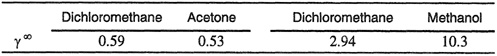
These data show that binary mixtures of dichloromethane/acetone exhibit appreciable negative deviations from Raoult’s law. However, the data for binary mixtures of dichloromethane/methanol exhibit large positive deviations. Why is there such a striking difference between these two binary systems?

(b) At 50°C, we have data for the activity coefficient of nitroethane in benzene and in hexane. When the mole fraction of nitroethane is 0.05, is the activity coefficient of nitroethane larger in benzene or in hexane? Explain.

(c) Near room temperature, we want to dissolve a heavy, aromatic, coal-derived liquid in a volatile solvent. Two solvents are considered: methane! and chloroform. Which solvent is better; that is, in which solvent is the solute likely to be more soluble? Why?