![]()
Integration
In this chapter we cover different aspects of integration, with the main focus on numerical integration. For historical reasons, numerical integration is also known as quadrature. Integration is significantly more difficult than its inverse operation – differentiation – and while there are many examples of integrals that can be calculated symbolically, in general we have to resort to numerical methods. Depending on the properties of the integrand (the function being integrated) and the integration limits, it can be easy or difficult to numerically compute an integral. Integrals of continuous functions and with finite integration limits can in most cases be computed efficiently in one dimension, but integrable functions with singularities or integrals with infinite integration limits are examples of cases that can be difficult to handle numerically, even in a single dimension. Double integrals and higher-order integrals can be numerically computed with repeated single-dimension integration, or using methods that are multidimensional generalizations of the techniques used to solve single-dimensional integrals. However, the computational complexity grows quickly with the number of dimensions to integrate over, and in practice such methods are only feasible for low-dimensional integrals, such as double integrals or triple integrals. Integrals of higher dimension than that often require completely different techniques, such as Monte Carlo sampling algorithms.
In addition to numerical evaluation of integrals with definite integration limits, which gives a single number as the result, integration also has other important applications. For example, equations where the integrand of an integral is the unknown quantity are called integral equations, and such equations frequently appear in science and engineering applications. Integral equations are usually difficult to solve, but they can often be recast into linear equation systems by discretizing the integral. However, we do not cover this topic here, but we will see examples of this type of problem in Chapter 11. Another important application of integration is integral transforms, which are techniques for transforming functions and equations between different domains. At the end of this chapter we briefly discuss how SymPy can be used to compute some integral transforms, such as Laplace transforms and Fourier transforms.
To carry out symbolic integration we can use SymPy, as briefly discussed in Chapter 3, and to compute numerical integration we mainly use the integrate module in SciPy. However, SymPy (through the multiple-precision library mpmath) also have routines for numerical integration, which complement those in SciPy, for example, by offering arbitrary-precision integration. In this chapter we look into both these options and discuss their pros and cons. We also briefly look at Monte Carlo integrations using the scikit-monaco library.
![]() Scikit-monaco Scikit-monaco is a small and recent library that makes Monte Carlo integration convenient and easily accessible. At the time of writing, the most recent version of scikit-monaco is 0.2.1. See http://scikit-monaco.readthedocs.org for more information.
Scikit-monaco Scikit-monaco is a small and recent library that makes Monte Carlo integration convenient and easily accessible. At the time of writing, the most recent version of scikit-monaco is 0.2.1. See http://scikit-monaco.readthedocs.org for more information.
Importing Modules
In this chapter we require, as usual, the NumPy and the Matplotlib libraries for basic numerical and plotting support, and on top of that we use the integrate module from SciPy and the SymPy library. Here we assume that these modules are imported as follows:
In [1]: import numpy as np
In [2]: import matplotlib.pyplot as plt
In [3]: from scipy import integrate
In [4]: import sympy
In addition, for nicely formatted output from SymPy, we also need to set up its printing system:
In [5]: sympy.init_printing()
Numerical Integration Methods
Here we are concerned with evaluating definite integrals on the form 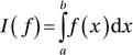 , with given integration limits a and b. The interval [a, b] can be finite, semi-infinite (where either
 ![]() or
or ![]() ), or infinite (where
), or infinite (where ![]() and
and ![]() ). The integral I(f ) can be interpreted as the area between the curve of the integrand f (x) and the x axis, as illustrated in Figure 8-1.
). The integral I(f ) can be interpreted as the area between the curve of the integrand f (x) and the x axis, as illustrated in Figure 8-1.

Figure 8-1. Interpretation of an integral as the area between the curve of the integrand and the x axis, where the area is counted as positive where ![]() (green) and negative otherwise (red)
(green) and negative otherwise (red)
A general strategy for numerically evaluating an integral I(f ), on the form given above, is to write the integral as a discrete sum that approximates the value of the integral:
![]()
Here wi are the weights of n evaluations of f (x) at the points ![]() , and rn is the residual due to the approximation. In practice we assume that rn is small and can be neglected, but it is important to have an estimate of rn to known how accurately the integral is approximated. This summation formula for I(f ) is known as a n-point quadrature rule, and the choice of the number of points n, their locations in [a, b], and the weight factors wi influence the accuracy and the computational complexity of its evaluation. Quadrature rules can be derived from interpolations of f (x) on the interval [a, b]. If the points xi are evenly spaced in the interval [a, b], and a polynomial interpolation is used, then the resulting quadrature rule is known as a Newton-Cotes quadrature rule. For instance, approximating f (x) with a zeroth order polynomial (constant value) using the midpoint value
, and rn is the residual due to the approximation. In practice we assume that rn is small and can be neglected, but it is important to have an estimate of rn to known how accurately the integral is approximated. This summation formula for I(f ) is known as a n-point quadrature rule, and the choice of the number of points n, their locations in [a, b], and the weight factors wi influence the accuracy and the computational complexity of its evaluation. Quadrature rules can be derived from interpolations of f (x) on the interval [a, b]. If the points xi are evenly spaced in the interval [a, b], and a polynomial interpolation is used, then the resulting quadrature rule is known as a Newton-Cotes quadrature rule. For instance, approximating f (x) with a zeroth order polynomial (constant value) using the midpoint value ![]() , we obtain
, we obtain

This is known as the midpoint rule, and it integrates polynomials of up to order one (linear functions) exactly, and it is therefore said to be of polynomial degree one. Approximating f (x) by a polynomial of degree one, evaluated at the endpoints of the interval, results in

This is known as the trapezoid rule, and it is also of polynomial degree one. Using an interpolation polynomial of second order results in Simpson’s rule,
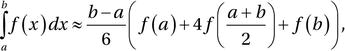
which uses function evaluations at the endpoints and the midpoint. This method is of polynomial degree three, meaning that it integrates exactly polynomials up to order three. The method of arriving at this formula can easily be demonstrated using SymPy: first we define symbols for the variables a, b, and x, as well as the function f.
In [6]: a, b, X = sympy.symbols("a, b, x")
In [7]: f = sympy.Function("f")
Next we define a tuple x that contains the sample points (the endpoints and the middle point of the interval [a, b]), and a list w of weight factors to be used in the quadrature rule, corresponding to each sample point:
In [8]: x = a, (a+b)/2, b  # for Simpson’s rule
In [9]: w = [sympy.symbols("w_%d" % i) for i in range(len(x))]
Given x and w we can now construct a symbolic expression for the quadrature rule:
In [10]: q_rule = sum([w[i] * f(x[i]) for i in range(len(x))])
In [11]: q_rule
Out[11]:
To compute the appropriate values of the weight factors wi we choose the polynomial basis functions
![]() for the interpolation of f (x), and here we use the sympy.Lambda function to create symbolic representations for each of these basis functions:
for the interpolation of f (x), and here we use the sympy.Lambda function to create symbolic representations for each of these basis functions:
In [12]: phi = [sympy.Lambda(X, X**n) for n in range(len(x))]
In [13]: phi
Out[13]:
The key to finding the quadrature weight factors is that the integral  can be computed analytically for each of basis functions øn(x). By substituting the function f (x) with each of the basis functions øn(x) in the quadrature rule, we obtain an equation system for the unknown weight factors:

These equations are equivalent to requiring that the quadrature rule exactly integrates all the basis functions, and therefore also (at least) all functions that are spanned by the basis. The equation system can be constructed with SymPy using:
In [14]: eqs = [q_rule.subs(f, phi[n]) - sympy.integrate(phi[n](X), (X, a, b))
    ...:        for n in range(len(phi))]
In [15]: eqs
Out[15]:
Solving this linear equation system gives analytical expressions for the weight factors:
In [16]: w_sol = sympy.solve(eqs, w)
In [17]: w_sol
Out[17]:
and by substituting the solution into the symbolic expression for the quadrature rule we obtain:
In [18]: q_rule.subs(w_sol).simplify()
Out[18]:
We recognize this result as Simpson’s quadrature rule given above. Choosing different sample points (the x tuple in this code), results in different quadrature rules.
Higher-order quadrature rules can similarly be derived using higher-order polynomial interpolation (more sample points in the [a, b] interval). However, high-order polynomial interpolation can have undesirable behavior between the sample points, as discussed in Chapter 7. Rather than using higher-order quadrature rules it is therefore often better to divide the integration interval [a, b] into subintervals ![]() , and use a low-order quadrature rule in each of these subintervals. Such methods are known as composite quadrature rules. Figure 8-2 shows the three lowest order Newton-Cotes quadrature rules for the function
, and use a low-order quadrature rule in each of these subintervals. Such methods are known as composite quadrature rules. Figure 8-2 shows the three lowest order Newton-Cotes quadrature rules for the function ![]() on the interval
on the interval ![]() , and the corresponding composite quadrature rules with four subdivisions of the original interval.
, and the corresponding composite quadrature rules with four subdivisions of the original interval.

Figure 8-2. Vizualization of quadature rules (top panel) and composite quadrature rules (bottom panel) of order zero (the midpoint rule), one (the Trapezoid rule) and two (Simpon’s rule)
An important parameter that characterize composite quadrature rules is the subinterval length ![]() . Estimates for the errors in an approximate quadrature rule, and the scaling of the error with respect to h, can be obtained from Taylor series expansions of the integrand and the analytical integration of the term in the resulting series. An alternative technique is to simultaneously consider quadrature rules of different order, or of different subinterval length h. The difference between two such results can often be shown to give estimates of the error, and this is the basis for how many quadrature routines produce an estimate of the error in addition to the estimate of the integral, as we will see examples of in the following section.
. Estimates for the errors in an approximate quadrature rule, and the scaling of the error with respect to h, can be obtained from Taylor series expansions of the integrand and the analytical integration of the term in the resulting series. An alternative technique is to simultaneously consider quadrature rules of different order, or of different subinterval length h. The difference between two such results can often be shown to give estimates of the error, and this is the basis for how many quadrature routines produce an estimate of the error in addition to the estimate of the integral, as we will see examples of in the following section.
We have seen that the Newton-Cotes quadrature rules uses evenly spaced sample points of the integrand f (x). This is often convenient, especially if the integrand is obtained from measurements or observations at prescribed points, and cannot be evaluated at arbitrary points in the interval [a, b]. However, this is not necessarily the most efficient choice of quadrature nodes, and if the integrand is given as a function that easily can be evaluated at arbitrary values of ![]() , then it can be advantageous to use quadrature rules that do not use evenly spaced sample points. An example of such a method is a Gaussian quadrature, which also uses polynomial interpolation to determine the values of the weight factors in the quadrature rule, but where the quadrature nodes xi are chosen to maximize the order of polynomials that can be integrated exactly (the polynomial degree) given a fixed number of quadrature points. It turns out that choices xi that satisfy this critera are the roots of different orthogonal polynomials, and the sample points xi are typically located at irrational locations in the integration interval [a, b]. This is typically not a problem for numerical implementations, but practically it requires that the function f (x) is available to be evaluated at arbitrary points that are decided by the integration routine, rather than given as tabulated or precomputed data at regularly spaced x values. Guassian quadrature rules are typically superior if f (x) can be evaluated at arbitrary values, but for the reason just mentioned, the Newton-Cotes quadrature rules also have important use-cases when the integrand is given as tabulated data.
, then it can be advantageous to use quadrature rules that do not use evenly spaced sample points. An example of such a method is a Gaussian quadrature, which also uses polynomial interpolation to determine the values of the weight factors in the quadrature rule, but where the quadrature nodes xi are chosen to maximize the order of polynomials that can be integrated exactly (the polynomial degree) given a fixed number of quadrature points. It turns out that choices xi that satisfy this critera are the roots of different orthogonal polynomials, and the sample points xi are typically located at irrational locations in the integration interval [a, b]. This is typically not a problem for numerical implementations, but practically it requires that the function f (x) is available to be evaluated at arbitrary points that are decided by the integration routine, rather than given as tabulated or precomputed data at regularly spaced x values. Guassian quadrature rules are typically superior if f (x) can be evaluated at arbitrary values, but for the reason just mentioned, the Newton-Cotes quadrature rules also have important use-cases when the integrand is given as tabulated data.
Numerical Integration with SciPy
The numerical quadrature routines in the SciPy integrate module can be categorized into two types: routines that take the integrand as a Python function, and routines that take arrays with samples of the integrand at given points. The functions of the first type use Gaussian quadrature (quad, quadrature, fixed_quad), while functions of the second type use Newton-Cotes methods (trapz, simps, and romb).
The quadrature function is an adaptive Gaussian quadrature routine that is implemented in Python. The quadrature repeatedly calls the fixed_quad function, for Gaussian quadrature of fixed order, with increasing order until the required accuracy is reached. The quad function is a wrapper for routines from the FORTRAN library QUADPACK, which has superior performance and more features (such as support for infinite integration limits). It is therefore usually preferable to use quad, and in the following we use this quadrature function. However, all these functions take similar arguments and can often be replaced with each other. They take as a first argument the function that implements the integrand, and the second and third arguments are the lower and upper integration limits. As a concrete example, consider the numerical evaluation of the integral ![]() . To evaluate this integral using SciPy’s quad function, we first define a function for the integrand and then call the quad function:
. To evaluate this integral using SciPy’s quad function, we first define a function for the integrand and then call the quad function:
In [19]: def f(x):
    ...:     return np.exp(-x**2)
In [20]: val, err = integrate.quad(f, -1, 1)
In [21]: val
Out[21]: 1.493648265624854
In [22]: err
Out[22]: 1.6582826951881447e−14
The quad function returns a tuple that contains the numerical estimate of the integral, val; and an estimate of the absolute error, err, in the integral value. The tolerances for the absolute and the relative errors can be set using the optional epsabs and epsrel keyword arguments, respectively. If the function f takes more than one variable, the quad routine integrates the function over its first argument. We can optionally specify the values of additional arguments by passing those values to the integrand function via the keyword argument args to the quad function. For example, if we wish to evaluate ![]() for the specific values of the parameters
for the specific values of the parameters ![]() ,
, ![]() , and
, and ![]() , we can define a function for the integrand that takes all these additional arguments, and then specify the values of a, b, and c by passing args=(1, 2, 3) to the quad function:
, we can define a function for the integrand that takes all these additional arguments, and then specify the values of a, b, and c by passing args=(1, 2, 3) to the quad function:
In [23]: def f(x, a, b, c):
    ...:     return a * np.exp(-((x - b)/c)**2)
In [24]: val, err = integrate.quad(f, -1, 1, args=(1, 2, 3))
In [25]: val
Out[25]: 1.2763068351022229
In [26]: err
Out[26]: 1.4169852348169507e−14
When working with functions where the variable we want to integrate over is not the first argument, we can reshuffle the arguments by using a lambda function. For example, if we wish to compute the integral
![]() , where the integrand J0(x) is the zeroth order Bessel function of the first kind, it would be convenient to use the function jv from the scipy.special module as integrand. The function jv takes the arguments v and x, and is the Bessel function of the first kind for the real-valued order v and evaluated at x. To be able to use the jv function as integrand for quad, we there need to reshuffle the arguments of jv. With a lambda function, we can do this in the following manner:
, where the integrand J0(x) is the zeroth order Bessel function of the first kind, it would be convenient to use the function jv from the scipy.special module as integrand. The function jv takes the arguments v and x, and is the Bessel function of the first kind for the real-valued order v and evaluated at x. To be able to use the jv function as integrand for quad, we there need to reshuffle the arguments of jv. With a lambda function, we can do this in the following manner:
In [27]: from scipy.special import jv
In [28]: f = lambda x: jv(0, x)
In [29]: val, err = integrate.quad(f, 0, 5)
In [30]: val
Out[30]: 0.7153119177847678
In [31]: err
Out[31]: 2.47260738289741e−14
With this technique we can arbitrarily reshuffle arguments of any function, and always obtain a function where the integration variable is the first argument, so that the function can be used as integrand for quad.
The quad routine supports infinite integration limits. To represent integration limits that are infinite, we use the floating-point representation of infinity, float('inf'), which is conveniently available in NumPy as
np.inf. For example, consider the integral ![]() . To evaluate it using quad we can do:
. To evaluate it using quad we can do:
In [32]: f = lambda x: np.exp(-x**2)
In [33]: val, err = integrate.quad(f, -np.inf, np.inf)
In [34]: val
Out[34]: 1.7724538509055159
In [35]: err
Out[35]: 1.4202636780944923e−08
However, note that the quadrature and fixed_quad functions only support finite integration limits.
With a bit of extra guidance, the quad function is also able to handle many integrals with integrable singularities. For example, consider the integral  . The integrand diverges at
 ![]() , but the value of the integral does not diverge, and its value is 4. Naively trying to compute this integral using quad may fail because of the diverging integrand:
, but the value of the integral does not diverge, and its value is 4. Naively trying to compute this integral using quad may fail because of the diverging integrand:
In [36]: f = lambda x: 1/np.sqrt(abs(x))
In [37]: a, b = -1, 1
In [38]: integrate.quad(f, a, b)
Out[38]: (inf, inf)
In situations like these, it can be useful to graph the integrand to get insights into how it behaves, as shown in Figure 8-3.
In [39]: fig, ax = plt.subplots(figsize=(8, 3))
    ...: x = np.linspace(a, b, 10000)
    ...: ax.plot(x, f(x), lw=2)
    ...: ax.fill_between(x, f(x), color='green', alpha=0.5)
    ...: ax.set_xlabel("$x$", fontsize=18)
    ...: ax.set_ylabel("$f(x)$", fontsize=18)
    ...: ax.set_ylim(0, 25)

Figure 8-3. Example of a diverging integrand with finite integral (green/shaded area) that can be computed using the quad function
In this case the evaluation of the integral fails because the integrand diverges exactly at one of the sample points in the Gaussian quadrature rule (the midpoint). We can guide the quad routine by specifying a list of points that should be avoided using the points keyword arguments, and using points=[0] in the current example allows quad to correctly evaluate the integral:
In [40]: integrate.quad(f, a, b, points=[0])
Out[40]: (4.0,5.684341886080802e−14)
We have seen that the quad routine is suitable for evaluating integrals when the integrand is specified using a Python function that the routine can evaluate at arbitrary points (which is determined by the specific quadrature rule). However, in many situations we may have an integrand that is only specified at predetermined points, such as evenly spaced points in the integration interval [a, b]. This type of situation can occur, for example, when the integrand is obtained from experiments or observations that cannot realistically be controlled by the particular integration routine. In this case we can use the Newton-Cotes quadrature, such as the midpoint rule, trapezoid rule, or Simpson’s rule that were described earlier in this chapter.
In the SciPy integrate module the composite trapezoid rule and Simpson’s rule are implemented in the trapz and simps functions. These functions take as first argument an array y with values of the integrand at a set of points in the integration interval, and they optionally take as second argument an array x that specifies the x values of the sample points, or alternatively the spacing dx between each sample (if uniform). Note that the sample points do not necessarily need to be evenly spaced, but they must be determined and evaluated in advance.
To see how to evaluate an integral of a function that is given by sampled values, let’s evaluate the integral  by taking 25 samples of the integrand in the integration interval [0, 2], as shown in Figure 8-4:
In [41]: f = lambda x: np.sqrt(x)
In [42]: a, b = 0, 2
In [43]: x = np.linspace(a, b, 25)
In [44]: y = f(x)
In [45]: fig, ax = plt.subplots(figsize=(8, 3))
    ...: ax.plot(x, y, 'bo')
    ...: xx = np.linspace(a, b, 500)
    ...: ax.plot(xx, f(xx), 'b-')
    ...: ax.fill_between(xx, f(xx), color='green', alpha=0.5)
    ...: ax.set_xlabel(r"$x$", fontsize=18)
    ...: ax.set_ylabel(r"$f(x)$", fontsize=18)
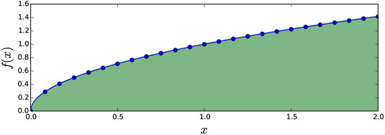
Figure 8-4. Integrad given as tabulated values marked with dots. The integral corresponds to the shaded area
To evaluate the integral we can pass the x and y arrays to the trapz or simps methods. Note that the y array must be passed as the first argument:
In [46]: val_trapz = integrate.trapz(y, x)
In [47]: val_trapz
Out[47]: 1.88082171605
In [48]: val_simps = integrate.simps(y, x)
In [49]: val_simps
Out[49]: 1.88366510245
The trapz and simps functions do not provide any error estimates, but for this particular example we can compute the integral analytically and compare to the numerically values computed width the two methods:
In [50]: val_exact = 2.0/3.0 * (b-a)**(3.0/2.0)
In [51]: val_exact
Out[51]: 1.8856180831641267
In [52]: val_exact - val_trapz
Out[52]: 0.00479636711328
In [53]: val_exact - val_simps
Out[53]: 0.00195298071541
Since all information we have about the integrand is the given sample points, we also cannot ask either of trapz and simps to compute more accurate solutions. The only option for increasing the accuracy is to increase the number of sample points, or use a higher-order method.
The integrate module also provides an implementation of the Romberg method with the romb function. The Romberg method is a Newton-Cotes method, but one that uses Richardson extrapolation to accelerate the convergence of the trapezoid method, however this method do require that the sample points are evenly spaced, and also that there are ![]() sample points, where n is an integer. Like the trapz and simps methods, romb takes an array with integrand samples as first argument, but the second argument must (if given) be the sample-point spacing dx:
sample points, where n is an integer. Like the trapz and simps methods, romb takes an array with integrand samples as first argument, but the second argument must (if given) be the sample-point spacing dx:
In [54]: x = np.linspace(a, b, 1 + 2**6)
In [55]: len(x)
Out[55]: 65
In [56]: y = f(x)
In [57]: dx = x[1] - x[0]
In [58]: val_exact - integrate.romb(y, dx=dx)
Out[58]: 0.000378798422913
Among these functions, simps is perhaps overall the most useful one, since it provides a good balance between ease of use (no constraint on the sample points) and relatively good accuracy.
Multiple Integration
Multiple integrals, such as double integrals  and triple integrals
  , can be evaluated using the dblquad and tplquad functions from the SciPy integrate module. Also, integration over n variables
 ![]() , over some domain D, can be evaluated using the nquad function. These functions are wrappers around the single-variable quadrature function quad, which is called repeatedly along each dimension of the integral.
, over some domain D, can be evaluated using the nquad function. These functions are wrappers around the single-variable quadrature function quad, which is called repeatedly along each dimension of the integral.
Specifically, the double integral routine dblquad can evaluate integrals on the form

and it has the function signature dblquad(f, a, b, g, h), where f is a Python function for the integrand, a and b are constant integration limits along the x dimension, and g and f are Python functions (taking x as argument) that specify the integration limits along the y dimension. For example, consider the integral
![]() . To evaluate this we first define the function f for the integrand and graph the function and the integration region, as shown in Figure 8-5:
. To evaluate this we first define the function f for the integrand and graph the function and the integration region, as shown in Figure 8-5:
In [59]: def f(x, y):
    ...:     return np.exp(-x**2 - y**2)
In [60]: fig, ax = plt.subplots(figsize=(6, 5))
    ...: x = y = np.linspace(-1.25, 1.25, 75)
    ...: X, Y = np.meshgrid(x, y)
    ...: c = ax.contour(X, Y, f(X, Y), 15, cmap=mpl.cm.RdBu, vmin=-1, vmax=1)
    ...: bound_rect = plt.Rectangle((0, 0), 1, 1, facecolor="grey")
    ...: ax.add_patch(bound_rect)
    ...: ax.axis('tight')
    ...: ax.set_xlabel('$x$', fontsize=18)
    ...: ax.set_ylabel('$y$', fontsize=18)

Figure 8-5. Two-dimensional integrand as contour plot with integration region shown as a shaded area
In this example the integration limits for both the x and y variables are constants, but since dblquad expects functions for the integration limits for the y variable, we must also define the functions h and g, even though in this case they only evaluate to constants regardless of the value of x.
In [61]: a, b = 0, 1
In [62]: g = lambda x: 0
In [63]: h = lambda x: 1
Now, with all the arguments prepared, we can call dblquad to evaluate the integral:
In [64]: integrate.dblquad(f, a, b, g, h)
Out[64]: (0.5577462853510337, 6.1922276789587025e−15)
Note that we could also have done the same thing a bit more concisely, although slightly less readably, by using inline lambda function definitions:
In [65]: integrate.dblquad(lambda x, y: np.exp(-x**2-y**2), 0, 1, lambda x: 0, lambda x: 1)
Out[65]: (0.5577462853510337, 6.1922276789587025e−15)
Due to that g and h are functions, we can compute integrals with x-dependent integration limits along the y dimension. For example, with ![]() and
and ![]() , we obtain:
, we obtain:
In [66]: integrate.dblquad(f, 0, 1, lambda x: -1 + x, lambda x: 1 - x)
Out[66]: (0.7320931000008094, 8.127866157901059e−15)
The tplquad function can compute integrals on the form

which is a generalization of the double integral expression computed with dblquad. It additionally takes two Python functions as arguments, which specifies the integration limits along the z dimension. These functions takes two arguments, x and y, but note that g and h still only takes one argument (x). To see how tplquad can be used, consider the generalization of the previous integral to three variables:
![]() . We compute this integral using a similar method compared to the dblquad example. That is, we first define functions for the integrand and the integration limits, and the call the tplquad function:
. We compute this integral using a similar method compared to the dblquad example. That is, we first define functions for the integrand and the integration limits, and the call the tplquad function:
In [67]: def f(x, y, z):
    ...:    return np.exp(-x**2-y**2-z**2)
In [68]: a, b = 0, 1
In [69]: g, h = lambda x: 0, lambda x: 1
In [70]: q, r = lambda x, y: 0, lambda x, y: 1
In [71]: integrate.tplquad(f, 0, 1, g, h, q, r)
Out[71]: (0.4165383858866382,4.624505066515441e−15)
For arbitrary number of integrations, we can use the nquad function. It also takes the integrand as a Python function as first argument. The integrand function should have the function signature f(x1, x2, ..., xn). In contrast to dplquad and tplquad, the nquad function expects list of integration limit specifications, as second argument. The list should contain a tuple with integration limits for each integration variable, or a callable function that returns such a limit. For example, to compute the integral that we previously computed with tplquad, we could use:
In [72]: integrate.nquad(f, [(0, 1), (0, 1), (0, 1)])
Out[72]: (0.4165383858866382, 8.291335287314424e−15)
For an increasing number of integration variables, the computational complexity of a multiple integral grows quickly, for example, when using nquad. To see this scaling trend, consider the following generalized version of the integrand studied with dplquad and tplquad.
In [73]: def f(*args):
    ...:    """
    ...:    f(x1, x2, ... , xn) = exp(-x1^2 - x2^2 - ... – xn^2)
    ...:    """
    ...:    return np.exp(-np.sum(np.array(args)**2))
Next, we evaluate the integral for varying number of dimensions (ranging from one up to five). In the following examples, the length of the list of integration limits determines the number of the integrals. To see a rough estimate of the computation time we use the IPython command %time:
In [74]: %time integrate.nquad(f, [(0,1)] * 1)
CPU times: user 398 μs, sys: 63 μs, total: 461 μs
Wall time: 466 μs
Out[74]: (0.7468241328124271,8.291413475940725e−15)
In [75]: %time integrate.nquad(f, [(0,1)] * 2)
CPU times: user 6.31 ms, sys: 298 μs, total: 6.61 ms
Wall time: 6.57 ms
Out[75]: (0.5577462853510337,8.291374381535408e−15)
In [76]: %time integrate.nquad(f, [(0,1)] * 3)
CPU times: user 123 ms, sys: 2.46 ms, total: 126 ms
Wall time: 125 ms
Out[76]: (0.4165383858866382,8.291335287314424e−15)
In [77]: %time integrate.nquad(f, [(0,1)] * 4)
CPU times: user 2.41 s, sys: 11.1 ms, total: 2.42 s
Wall time: 2.42 s
Out[77]: (0.31108091882287664,8.291296193277774e−15)
In [78]: %time integrate.nquad(f, [(0,1)] * 5)
CPU times: user 49.5 s, sys: 169 ms, total: 49.7 s
Wall time: 49.7 s
Out[78]: (0.23232273743438786,8.29125709942545e−15)
Here we see that increasing the number of integrations form one to five, increases the computation time from hundreds of microseconds to nearly a minute. For even larger number of integrals it may become impractical to use direct quadrature routines, and other methods, such as Monte Carlo sampling techniques can often be superior, especially if the required precision is not that high.
To compute an integral using Monte Carle sampling, we can use the mcquad function from the skmonaco library (known as scikit-monaco). As first argument it takes a Python function for the integrand, and as second argument it takes a list of lower integration limits, and as third argument it takes a list of upper integration limits. Note that the way the integration limits are specified is not exactly the same as for the quad function in SciPy’s integrate module. We begin by importing the skmonaco (Scikit-Monaco) module:
In [79]: import skmonaco
Once the module is imported, we can use the skmonaco.mcquad function for performing a Monte Carlo integration. In the following example we compute the same integral as in the previous example using nquad:
In [80]: %time val, err = skmonaco.mcquad(f, xl=np.zeros(5), xu=np.ones(5), npoints=100000)
CPU times: user 1.43 s, sys: 100 ms, total: 1.53 s
Wall time: 1.5 s
In [81]: val, err
Out[81]: (0.231322502809, 0.000475071311272)
While the error is not comparable to the result given by nquad, the computation time is much shorter. By increasing the number of sample points, which we can specify using the npoints argument, we can increase the accuracy of the result. However, the convergence of Monte Carlo integration is very slow, and it is most suitable when high accuracy is not required. However, the beauty of Monte Carlo integration is that its computational complexity is independent of the number of integrals. This is illustrated in the following example, which computes a 10-variable integration in the same time and with comparable error level as the previous example with a 5-variable integration:
In [82]: %time val, err = skmonaco.mcquad(f, xl=np.zeros(10), xu=np.ones(10), npoints=100000)
CPU times: user 1.41 s, sys: 64.9 ms, total: 1.47 s
Wall time: 1.46 s
In [83]: val, err
Out[83]: (0.0540635928549, 0.000171155166006)
Symbolic and Arbitrary-Precision Integration
In Chapter 3, we already saw examples of how SymPy can be used to compute definite and indefinite integrals of symbolic functions, using the sympy.integrate function. For example, to compute the integral
![]() , we first create a symbol for x, and define expressions for the integrand and the integration limits
, we first create a symbol for x, and define expressions for the integrand and the integration limits ![]() and
and![]() :
:
In [84]: x = sympy.symbols("x")
In [85]: f = 2 * sympy.sqrt(1-x**2)
In [86]: a, b = -1, 1
after which we can compute the closed-form expression for the integral using:
In [87]: val_sym = sympy.integrate(f, (x, a, b))
In [88]: val_sym
Out[88]: π
For this example, SymPy is able to find the analytic expression for the integral: π. As pointed out earlier, this situation is the exception, and in general we will not be able to find an analytical closed-form expression. We then need to resort to numerical quadrature, for example, using SciPy’s integrate.quad, as discussed earlier in this chapter. However, the mpmath library,1 which comes bundled with SymPy, or which can be installed and imported on its own, provides an alternative implementation of numerical quadrature, using multiple-precision computations. With this library, we can evaluate an integral to arbitrary precision, without being restricted to the limitations of floating-point numbers. However, the downside is, of course, that arbitrary-precision computations are significantly slower than float-point computations. But when we require precision beyond what the SciPy quadrature functions can provide, this multiple-precision quadrature provides a solution.
For example, to evaluate the integral ![]() to a given precision,2 we can use the sympy.mpmath.quad function, which takes a Python function for the integrand as first argument, and the integration limits as a tuple (a, b) as second argument. To specify the precision, we set the variable sympy.mpmath.mp.dps to the required number of accurate decimal places. For example, if we require 75 accurate decimal places, we set:
to a given precision,2 we can use the sympy.mpmath.quad function, which takes a Python function for the integrand as first argument, and the integration limits as a tuple (a, b) as second argument. To specify the precision, we set the variable sympy.mpmath.mp.dps to the required number of accurate decimal places. For example, if we require 75 accurate decimal places, we set:
In [89]: sympy.mpmath.mp.dps = 75
The integrand must be given as a Python function that uses math functions from the mpmath library to compute the integrand. From a SymPy expression, we can create such a function using sympy.lambdify with 'mpmath' as third argument, which indicates that we want an mpmath compatible function. Alternatively, we can directly implement a Python function using the math functions from the mpmath module in SymPy, which in this case would be f_mpmath = lambda x: 2 * sympy.mpmath.sqrt(1 - x**2). However, here we use sympy.lambdify to automate this step:
In [90]: f_mpmath = sympy.lambdify(x, f, 'mpmath')
Next we can compute the integral using sympy.mpmath.quad, and display the resulting value:
In [91]: val = sympy.mpmath.quad(f_mpmath, (a, b))
In [92]: sympy.sympify(val)
Out[92]: 3.14159265358979323846264338327950288419716939937510582097494459230781640629
To verify that the numerically computed value is accurate to the required number of decimal places (75), we compare the result with the known analytical value (π). The error is indeed very small:
In [93]: sympy.N(val_sym, sympy.mpmath.mp.dps+1) - val
Out[93]: 6.90893484407555570030908149024031965689280029154902510801896277613487344253e−77
This level of precision cannot be achieved with the quad function in SciPy’s integrate module, since it is limited by the precision of floating-point numbers.
The mpmath library’s quad function can also be used to evaluate double and triple integrals. To do so, we only need to pass to it an integrand function that takes multiple variables as arguments, and pass tuples with integration limits for each integration variable. For example, to compute the double integral
![]()
and the triple integral
![]()
to 30 significant decimals (this example cannot be solved symbolically with SymPy), we could first create SymPy expressions for the integrands, and then use sympy.lambdify to create the corresponding mpmath expressions:
In [94]: x, y, z = sympy.symbols("x, y, z")
In [95]: f2 = sympy.cos(x) * sympy.cos(y) * sympy.exp(-x**2 - y**2)
In [96]: f3 = sympy.cos(x) * sympy.cos(y) * sympy.cos(z) * sympy.exp(-x**2 - y**2 - z**2)
In [97]: f2_mpmath = sympy.lambdify((x, y), f2, 'mpmath')
In [98]: f3_mpmath = sympy.lambdify((x, y, z), f3, 'mpmath')
The integrals can then be evaluated to the desired accuracy by setting sympy.mpmath.mp.dps and calling sympy.mpmath.quad:
In [99]: sympy.mpmath.mp.dps = 30
In [100]: sympy.mpmath.quad(f2_mpmath, (0, 1), (0, 1))
Out[100]: mpf('0.430564794306099099242308990195783')
In [101]: res = sympy.mpmath.quad(f3_mpmath, (0, 1), (0, 1), (0, 1))
In [102]: sympy.sympify(res)
Out[102]: 0.416538385886638169609660243601007
Again, this gives access to levels of accuracy that is beyond what scipy.integrate.quad can achieve, but this additional accuracy comes with a hefty increase in computational cost. Note that the type of the object returned by sympy.mpmath.quad is a multi-precision float (mpf). It can be cast into a SymPy type using sympy.sympify.
SymPy can also be used to compute line integrals on the form ![]() , where C is a curve in the x–y plane, using the line_integral function. This function takes the integrand, as a SymPy expression, as first argument, a sympy.Curve instance as second argument, and a list of integration variables as third argument. The path of the line integral is specified by the Curve instance, which describes a parameterized curve for which the x and y coordinates are given as a function of an independent parameter, say t. To create a Curve instance that describes a path along the unit circle, we can use:
, where C is a curve in the x–y plane, using the line_integral function. This function takes the integrand, as a SymPy expression, as first argument, a sympy.Curve instance as second argument, and a list of integration variables as third argument. The path of the line integral is specified by the Curve instance, which describes a parameterized curve for which the x and y coordinates are given as a function of an independent parameter, say t. To create a Curve instance that describes a path along the unit circle, we can use:
In [103]: t, x, y = sympy.symbols("t, x, y")
In [103]: C = sympy.Curve([sympy.cos(t), sympy.sin(t)], (t, 0, 2 * sympy.pi))
Once the integration path is specified, we can easily compute the corresponding line integral for a given integrand using line_integral. For example, with the integrand ![]() , the result is the circumference of the unit circle:
, the result is the circumference of the unit circle:
In [104]: sympy.line_integrate(1, C, [x, y])
Out[104]: 2π
The result is less obvious for a nontrivial integrand, such as in the following example where we compute the line integral with the integrand ![]() :
:
In [105]: sympy.line_integrate(x**2 * y**2, C, [x, y])
Out[105]: π/4
Integral Transforms
The last application of integrals that we discuss in this chapter is integral transforms. An integral transform is a procedure that takes a function as input and outputs another function. Integral transforms are the most useful when they can be computed symbolically, and here we explore two examples of integral transforms that can be performed using SymPy: the Laplace transform and the Fourier transform. There are numerous applications of these two transformations, but the fundamental motivation is to transform problems into a form that is more easily handled. It can, for example, be a transformation of a differential equation into an algebraic equation, using Laplace transforms, or a transformation of a problem from the time domain to the frequency domain, using Fourier transforms.
In general, an integral transform of a function f (t) can be written as
where Tf (u) is the transformed function. The choice of the kernel K(t, u) and the integration limits determines the type of integral transform. The inverse of the integral transform is given by

where ![]() is the kernel of the inverse transform. SymPy provides functions for several types of integral transform, but here we focus on the Laplace transform
is the kernel of the inverse transform. SymPy provides functions for several types of integral transform, but here we focus on the Laplace transform
![]()
with the inverse transform

and the Fourier transform
![]()
with the inverse transform
![]()
With SymPy, we can perform these transforms with the sympy.laplace_transform and sympy.fourier_transform, respectively, and the corresponding inverse transforms can be computed with the sympy.inverse_laplace_transform and sympy.inverse_fourier_transform. These functions take a SymPy expression for the function to transform as first argument, and the symbol for independent variable of the expression to transform as second argument (for example t), and as third argument they take the symbol for the transformation variable (for example s). For example, to compute the Laplace transformation of the function ![]() , we begin by defining SymPy symbols for the variables a, t, and s, and a SymPy expression for the function f (t):
, we begin by defining SymPy symbols for the variables a, t, and s, and a SymPy expression for the function f (t):
In [106]: s = sympy.symbols("s")
In [107]: a, t = sympy.symbols("a, t", positive=True)
In [108]: f = sympy.sin(a*t)
Once we have SymPy objects for the variables and the function, we can call the laplace_transform function to compute the Laplace transform:
In [109]: sympy.laplace_transform(f, t, s)
Out[109]: (,
,
)
By default, the laplace_transform function returns a tuple containing the resulting transform, the value A from convergence condition of the transform, which takes the form ![]() , and lastly additional conditions that are required for the transform to be well defined. These conditions typically depend on the constraints that are specified when symbols are created. For example, here we used positive=True when creating of the symbols a and t, to indicate that they represent real and positive numbers. Often we are only interested in the transform itself, and we can then use the noconds=True keyword argument to suppress the conditions in the return result:
, and lastly additional conditions that are required for the transform to be well defined. These conditions typically depend on the constraints that are specified when symbols are created. For example, here we used positive=True when creating of the symbols a and t, to indicate that they represent real and positive numbers. Often we are only interested in the transform itself, and we can then use the noconds=True keyword argument to suppress the conditions in the return result:
In [110]: F = sympy.laplace_transform(f, t, s, noconds=True)
In [111]: F
Out[111]:
The inverse transformation can be used in a similar manner, except that we need to reverse the roles of the symbols s and t. The Laplace transform is a unique one-to-one mapping, so if we compute the inverse Laplace transform of the previously computed Laplace transform we expect to recover the original function:
In [112]: sympy.inverse_laplace_transform(F, s, t, noconds=True)
Out[112]: sin(at)
SymPy can compute the transforms for many elementary mathematical functions, and for wide variety of combinations of such functions. When solving problems using Laplace transformations by hand, one typically searches for matching functions in reference tables with known Laplace transformations. Using SymPy, this process can conveniently be automated in many, but not all, cases. The following examples show a few additional examples of well-known functions that one find in Laplace transformation tables. Polynomials have simple Laplace transformation:
In [113]: [sympy.laplace_transform(f, t, s, noconds=True) for f in [t, t**2, t**3, t**4]]
Out[113]: [,
,
,
]
and we can also compute the general result with an arbitrary integer exponent:
In [114]: n = sympy.symbols("n", integer=True, positive=True)
In [115]: sympy.laplace_transform(t**n, t, s, noconds=True)
Out[115]:
The Laplace transform of composite expressions can also be computed, as in the following example that computes the transform of the function ![]() :
:
In [116]: sympy.laplace_transform((1 - a*t) * sympy.exp(-a*t), t, s, noconds=True)
Out[116]:
The main application of Laplace transforms is to solve differential equations, where the transformation can be used to bring the differential equation into a purely algebraic form, which can then be solved and transformed back to the original domain by applying the inverse Laplace transform. In Chapter 9 we will see concrete examples of this method. Fourier transforms can also be used for the same purpose.
The Fourier transform function, fourier_tranform, and its inverse, inverse_fourier_transform, are used in much the same way as the Laplace transformation functions. For example, to compute the Fourier transform of ![]() , we would first define SymPy symbols for the variables a, t, and ω, and the function f (t), and then compute the Fourier transform by calling the sympy.fourier_transform function:
, we would first define SymPy symbols for the variables a, t, and ω, and the function f (t), and then compute the Fourier transform by calling the sympy.fourier_transform function:
In [117]: a, t, w = sympy.symbols("a, t, omega")
In [118]: f = sympy.exp(-a*t**2)
In [119]: F = sympy.fourier_transform(f, t, w)
In [120]: F
Out[120]:
As expected, computing the inverse transformation for F recovers the original function:
In [121]: sympy.inverse_fourier_transform(F, w, t)
Out[121]:
SymPy can be used to compute a wide range of Fourier transforms symbolically, but unfortunately it does not handle well transformations that involve Dirac delta functions, in either the original function or the resulting transformation. This currently limits its usability, but nonetheless, for problems that do not involve Dirac delta functions it is a valuable tool.
Summary
Integration is one of the fundamental operations in mathematical analysis. Numerical quadrature, or numerical evaluation of integrals, have important applications in many fields of science, because integrals that occur in practice often cannot be computed analytically, and expressed as a closed-form expression. Their computation then requires numerical techniques. In this chapter we have reviewed basic techniques and methods for numerical quadrature, and introduced the corresponding functions in the SciPy integrate module that can be used for evaluation of integrals in practice. When the integrand is given as a function that can be evaluated at arbitrary points, we typically prefer Gaussian quadrature rules. On the other hand, when the integrand is defined as a tabulated data, the simpler Newton-Cotes quadrature rules can be used. We also studied symbolic integration and arbitrary-precision quadrature, which can complement floating-point quadrature for specific integrals that can be computed symbolically, or when additional precision is required. As usual, a good starting point is to begin to analyze a problem symbolically, and if a particular integral can be solved symbolically by finding its antiderivative, that is generally the most desirable situation. When symbolic integration fails, we need to resort to numerical quadrature, which should first be explored with floating-point based implementations, like the ones provided by the SciPy integrate module. If additional accuracy is required we can fall back on arbitrary-precision quadrature. Another application of symbolic integration is integral transform, which can be used to transform problems, such as differential equations, between different domains. Here we briefly looked at how to preform Laplace and Fourier transforms symbolically using SymPy, and in the following chapter we continue to explore this for solving certain types of differential equations.
Further Reading
Numerical quadrature is discussed in many introductory textbooks on numerical computing, such as those by Heath and Stoer. Detailed discussions on many quadrature methods, together with example implementations are available in a book by Press, Teukolsky, Vetterling, and Flannery. The theory of integral transforms, such as the Fourier transform and the Laplace transform is introduced in a book by Folland.
References
Folland, G. B. Fourier Analysis and Its Applications. American Mathematical Society, 1992.
Heath, M. T. Scientific Computing An Introductory Survey (2nd edition). New York: McGrawHill, 2002.
Press, W. H., Teukolsky, S. A., Vetterling, W. T, & Flannery, B. P. (2002). Numerical Recipes in C. Cambridge: Cambridge University Press, 2002.
Stoer, J., & Burlirsch, R. (1992). Introduction to Numerical Analysis. New York: Springer.
__________________
1For more information about the multi-precision (arbitrary precision) math library mpmath, see the project’s web page at http://mpmath.org.
2Here we deliberately choose to work with an integral that has a known analytical value, so that we can compare the multi-precision quadrature result with the known exact value.