
Chapter 1. Introduction to OpenGL
Chapter Objectives
After reading this chapter, you’ll be able to do the following:
• Describe the purpose of OpenGL, and what it can and cannot do in creating computer-generated images.
• Identify the common structure of an OpenGL application.
• Enumerate the shading stages that compose the OpenGL rendering pipeline.
This chapter introduces OpenGL. It has the following major sections:
• “What Is OpenGL?” explains what OpenGL is, what it does and doesn’t do, and how it works.
• “Your First Look at an OpenGL Program” provides a first look at what an OpenGL program looks like.
• “OpenGL Syntax” describes the format of the command names that OpenGL uses.
• “OpenGL’s Rendering Pipeline” discusses the processing pipeline that OpenGL uses in creating images.
• “Our First Program: A Detailed Discussion” dissects the first program presented and provides more detail on the activities of each section of the program.
What Is OpenGL?
OpenGL is an application programming interface, API for short, which is merely a software library for accessing features in graphics hardware. Version 4.5 of the OpenGL library (which this text covers) contains over 500 distinct commands that you use to specify the objects, images, and operations needed to produce interactive three-dimensional computer-graphics applications.
OpenGL is designed as a streamlined, hardware-independent interface that can be implemented on many different types of graphics hardware systems, or entirely in software (if no graphics hardware is present in the system), independent of a computer’s operating or windowing system. As such, OpenGL doesn’t include functions for performing windowing tasks or processing user input; instead, your application will need to use the facilities provided by the windowing system where the application will execute. Similarly, OpenGL doesn’t provide any functionality for describing models of three-dimensional objects, or operations for reading image files (JPEG files, for example). Instead, you must construct your three-dimensional objects from a small set of geometric primitives: points, lines, triangles, and patches.
Since OpenGL has been around a while—it was first developed at Silicon Graphics Computer Systems, with Version 1.0 released in July of 1994—there are many versions of OpenGL, as well as many software libraries built on OpenGL for simplifying application development, whether you’re writing a video game, creating a visualization for scientific or medical purposes, or just showing images. However, the more modern version of OpenGL differs from the original in significant ways. In this book, we describe how to use the most recent versions of OpenGL to create those applications.
The following list briefly describes the major operations that an OpenGL application would perform to render an image. (See “OpenGL’s Rendering Pipeline” on page 10 for detailed information on these operations.)
• Specify the data for constructing shapes from OpenGL’s geometric primitives.
• Execute various shaders to perform calculations on the input primitives to determine their position, color, and other rendering attributes.
• Convert the mathematical description of the input primitives into their fragments associated with locations on the screen. This process is called rasterization. (A fragment in OpenGL is what becomes a pixel, if it makes it all the way to the final rendered image.)
• Finally, execute a fragment shader for each of the fragments generated by rasterization, which will determine the fragment’s final color and position.
• Possibly perform additional per-fragment operations, such as determining if the object that the fragment was generated from is visible, or blending the fragment’s color with the current color in that screen location.
OpenGL is implemented as a client-server system, with the application you write being considered the client and the OpenGL implementation provided by the manufacturer of your computer graphics hardware being the server. In some implementations of OpenGL (such as those associated with the X Window System), the client and server might execute on different machines that are connected by a network. In such cases, the client will issue the OpenGL commands, which will be converted into a window-system specific protocol that is transmitted to the server via their shared network, where they are executed to produce the final image.
In most modern implementations, a hardware graphics accelerator is used to implement most of OpenGL and is either built into (but still separate form) the computer’s central processor, or it is mounted on a separate circuit board and plugged into the computer’s motherboard. In either case, it is reasonable to think of the client as your application and the server as the graphics accelerator.
Your First Look at an OpenGL Program
Because you can do so many things with OpenGL, an OpenGL program can potentially be large and complicated. However, the basic structure of all OpenGL applications is usually similar to the following:
1. Initialize the state associated with how objects should be rendered.
2. Specify those objects to be rendered.
Before you look at any code, let’s introduce some commonly used graphics terms. Rendering, which we’ve already used without defining, is the process by which a computer creates an image from models. OpenGL is just one example of a rendering system; there are many others. OpenGL is a rasterization-based system, but there are other methods for generating images as well, such as ray tracing, whose techniques are outside the scope of this book. However, even a system that uses ray tracing may employ OpenGL to display an image or compute information to be used in creating an image. Further, the flexibility available in recent versions of OpenGL has become so great that algorithms such as ray tracing, photon mapping, path tracing, and image-based rendering have become relatively easy to implement on programmable graphics hardware.
Our models, or objects—we’ll use the terms interchangeably—are constructed from geometric primitives: points, lines, and triangles, which are specified by their vertices.
Another concept that is essential to using OpenGL is shaders, which are special functions that the graphics hardware executes. The best way to think of shaders is as little programs that are specifically compiled for your graphics processing unit (GPU). OpenGL includes all the compiler tools internally to take the source code of your shader and create the code that the GPU needs to execute. In OpenGL, there are six shader stages that you can use. The most common are vertex shaders, which process vertex data, and fragment shaders, which operate on the fragments generated by the rasterizer.
The final generated image consists of pixels drawn on the screen; a pixel is the smallest visible element on your display. The pixels in your system are stored in a framebuffer, which is a chunk of memory that the graphics hardware manages and feeds to your display device.
Figure 1.1 shows the output of a simple OpenGL program, which renders two blue triangles into a window. The source code for the entire example is provided in Example 1.1.

Example 1.1 triangles.cpp: Our First OpenGL Program
//////////////////////////////////////////////////////////////////////
//
// triangles.cpp
//
//////////////////////////////////////////////////////////////////////
#include <iostream>
using namespace std;
#include "vgl.h"
#include "LoadShaders.h"
enum VAO_IDs { Triangles, NumVAOs };
enum Buffer_IDs { ArrayBuffer, NumBuffers };
enum Attrib_IDs { vPosition = 0 };
GLuint VAOs[NumVAOs];
GLuint Buffers[NumBuffers];
const GLuint NumVertices = 6;
//--------------------------------------------------------------------
//
// init
//
void
init(void)
{
static const GLfloat vertices[NumVertices][2] =
{
{ -0.90, -0.90 }, // Triangle 1
{ 0.85, -0.90 },
{ -0.90, 0.85 },
{ 0.90, -0.85 }, // Triangle 2
{ 0.90, 0.90 },
{ -0.85, 0.90 }
};
glCreateBuffers(NumBuffers, Buffers);
glNamedBufferStorage(Buffers[ArrayBuffer], sizeof(vertices),
vertices, 0);
ShaderInfo shaders[] = {
{ GL_VERTEX_SHADER, "triangles.vert" },
{ GL_FRAGMENT_SHADER, "triangles.frag" },
{ GL_NONE, NULL }
};
GLuint program = LoadShaders(shaders);
glUseProgram(program);
glGenVertexArrays(NumVAOs, VAOs);
glBindVertexArray(VAOs[Triangles]);
glBindBuffer(GL_ARRAY_BUFFER, Buffers[ArrayBuffer]);
glVertexAttribPointer(vPosition, 2, GL_FLOAT,
GL_FALSE, 0, BUFFER_OFFSET(0));
glEnableVertexAttribArray(vPosition);
}
//--------------------------------------------------------------------
//
// display
//
void
display(void)
{
static const float black[] = { 0.0f, 0.0f, 0.0f, 0.0f };
glClearBufferfv(GL_COLOR, 0, black);
glBindVertexArray(VAOs[Triangles]);
glDrawArrays(GL_TRIANGLES, 0, NumVertices);
}
//--------------------------------------------------------------------
//
// main
//
int
main(int argc, char** argv)
{
glfwInit();
GLFWwindow* window = glfwCreateWindow(640, 480, "Triangles", NULL,
NULL);
glfwMakeContextCurrent(window);
gl3wInit();
init();
while (!glfwWindowShouldClose(window))
{
display();
glfwSwapBuffers(window);
glfwPollEvents();
}
glfwDestroyWindow(window);
glfwTerminate();
}
While that may be more code than you were expecting, you’ll find that this program will be the basis of just about every OpenGL application you write. We use some additional software libraries that aren’t officially part of OpenGL to simplify things like creating a window, or receiving mouse or keyboard input—those things that OpenGL doesn’t include. We’ve also created some helper functions and small C++ classes to simplify our examples. While OpenGL is a C-language library, all of our examples are in C++, but very simple C++. In fact, most of the C++ we use is to implement the mathematical constructs vectors and matrices.
In a nutshell, here’s what Example 1.1 does. We’ll explain all of these concepts in complete detail later, so don’t worry.
• In the preamble of the program, we include the appropriate header files and declare global variables1 and other useful programming constructs.
1. Yes, in general we eschew global variables in large applications, but for the purposes of demonstration, we use them here.
• The init() routine is used to set up data for use later in the program. This may be vertex information for later use when rendering primitives or image data for use in a technique called texture mapping, which we describe in Chapter 6.
In this version of init(), we first specify the position information for the two triangles that we render. After that, we specify shaders we’re going to use in our program. In this case, we only use the required vertex and fragment shaders. The LoadShaders() routine is one that we’ve written to simplify the process of preparing shaders for a GPU. In Chapter 2 we’ll discuss everything it does.
The final part of init() is doing what we like to call shader plumbing, where you associate the data in your application with variables in shader programs. This is also described in detail in Chapter 2.
• The display() routine is what really does the rendering. That is, it calls the OpenGL functions that request something be rendered. Almost all display() routines will do the same three steps as in our simple example here.
1. Clear the window by calling glClearBufferfv().
2. Issue the OpenGL calls required to render your object.
3. Request that the image is presented to the screen.
• Finally, main() does the heavy lifting of creating a window, calling init(), and finally entering into the event loop. Here, you also see functions that begin with “gl” but look different than the other functions in the application. Those, which we’ll describe momentarily, are from the libraries we use to make it simple to write OpenGL programs across the different operating and window systems: GLFW, and GL3W.
Before we dive in to describe the routines in detail, let us explain OpenGL labels functions, constants, and other useful programming constructs.
OpenGL Syntax
As you likely picked up on, all the functions in the OpenGL library begin with the letters gl, immediately followed by one or more capitalized words to name the function (glBindVertexArray(), for example). All functions in OpenGL are like that. In the program you also saw the functions that began with glfw, which are from GLFW, which is a library that abstracts window management and other system tasks. Similarly, you see a single function, gl3wInit(), which comes from GL3W. We describe the GLFW library in more detail in Appendix A.
Similar to OpenGL’s function-naming convention, constants like GL_COLOR, which you saw in display(), are defined for the OpenGL library. All constant tokens begin with GL and use underscores to separate words. Their definitions are merely #defines found in the OpenGL header files: glcorearb.h and glext.h.
To aid in moving OpenGL applications between operating systems, OpenGL also defines various types of data for its functions, such as GLfloat, which is the floating-point value type we used to declare vertices in Example 1.1. OpenGL defines typedefs for all of the data types accepted by its functions, which are listed in Table 1.1. Additionally, because OpenGL is a C-language library, it doesn’t have function overloading to deal with the different types of data; it uses a function-naming convention to organize the multitude of functions that result from that situation. For example, we’ll encounter a function named glUniform*() in Chapter 2, “Shader Fundamentals,” which comes in numerous forms, such as glUniform2f() and glUniform3fv(). The suffixes at the end of the “core” part of the function name provide information about the arguments passed to the function. For example, the 2 in glUniform2f() represents that two data values will be passed into the function. (There are other parameters as well, but they are the same across all 24 versions of the glUniform*() function. In this book, we’ll use glUniform*() to represent the collection of all glUniform*() functions.) Also note the f following the 2. This indicates that those two parameters are of type GLfloat. Finally, some versions of the functions’ names end with a v, which is short for vector, meaning that the two floating-point values (in the case of glUniform2fv()) are passed as a one-dimensional array of GLfloats, instead of two separate parameters.
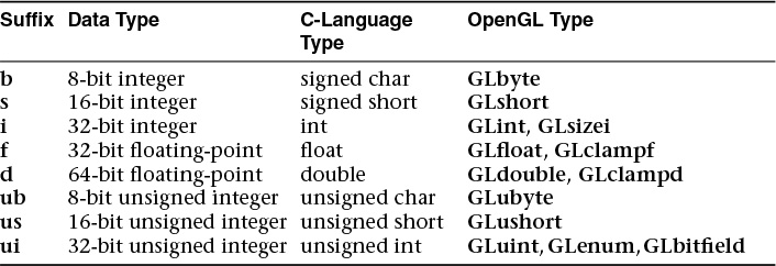
To decode all of those combinations, the letters used as suffixes are described in Table 1.1, along with their types.
Implementations of OpenGL have leeway in selecting which C data types to use to represent OpenGL data types. If you resolutely use the OpenGL-defined data types throughout your application, you will avoid mismatched types when porting your code between different implementations.
OpenGL’s Rendering Pipeline
OpenGL implements what’s commonly called a rendering pipeline, which is a sequence of processing stages for converting the data your application provides to OpenGL into a final rendered image. Figure 1.2 shows the OpenGL pipeline associated with Version 4.5. The OpenGL pipeline has evolved considerably since its introduction.

OpenGL begins with the geometric data you provide (vertices and geometric primitives) and first processes it through a sequence of shader stages—vertex shading, tessellation shading (which itself can use two shaders), and finally geometry shading—before it’s passed to the rasterizer. The rasterizer will generate fragments for any primitive that’s inside the clipping region and execute a fragment shader for each of the generated fragments.
As you can see, shaders play an essential role in creating OpenGL applications. You have complete control of which shader stages are used and what each of them do. Not all stages are required; in fact, only vertex shaders and fragment shaders must be included. Tessellation and geometry shaders are optional.
Now we dive deeper into each stage to provide you a bit more background. We understand that this may be a somewhat overwhelming at this point, but bear with us. It will turn out that understanding just a few concepts will get you very far along with OpenGL.
Preparing to Send Data to OpenGL
OpenGL requires that all data be stored in buffer objects, which are just chunks of memory managed by OpenGL. Populating these buffers with data can occur in numerous ways, but one of the most common is to specify the data at the same time as you specify the buffer’s size using the glNamedBufferStorage() command like in Example 1.1. There is some additional setup required with buffers, which we’ll cover in Chapter 3.
Sending Data to OpenGL
After we’ve initialized our buffers, we can request geometric primitives be rendered by calling one of OpenGL’s drawing commands, such as glDrawArrays(), as we did in Example 1.1.
Drawing in OpenGL usually means transferring vertex data to the OpenGL server. Think of a vertex as a bundle of data values that are processed together. While the data in the bundle can be anything you’d like it to be (i.e., you define all the data that makes up a vertex), it almost always includes positional data. Any other data will be values you’ll need to determine the pixel’s final color.
Drawing commands are covered in detail in Chapter 3, “Drawing with OpenGL.”
Vertex Shading
For each vertex that is issued by a drawing command, a vertex shader will be called to process the data associated with that vertex. Depending on whether any other pre-rasterization shaders are active, vertex shaders may be very simple, perhaps just copying data to pass it through this shading stage, what we call a pass-through shader, to a very complex shader that’s performing many computations to potentially compute the vertex’s screen position (usually using transformation matrices, described in Chapter 5), determining the vertex’s color using lighting computations described in Chapter 7, or any multitude of other techniques.
Typically, an application of any complexity will have multiple vertex shaders, but only one can be active at any one time.
Tessellation Shading
After the vertex shader has processed each vertex’s associated data, the tessellation shader stage will continue processing that data, if it’s been activated. As we’ll see in Chapter 9, tessellation uses patches to describe an object’s shape and allows relatively simple collections of patch geometry to be tessellated to increase the number of geometric primitives, providing better-looking models. The tessellation shading stage can potentially use two shaders to manipulate the patch data and generate the final shape.
Geometry Shading
The next shader stage, geometry shading, allows additional processing of individual geometric primitives, including creating new ones, before rasterization. This shading stage is optional but powerful, as we’ll see in Chapter 10.
Primitive Assembly
The previous shading stages all operate on vertices, with the information about how those vertices are organized into geometric primitives being carried along internal to OpenGL. The primitive assembly stage organizes the vertices into their associated geometric primitives in preparation for clipping and rasterization.
Clipping
Occasionally, vertices will be outside of the viewport—the region of the window where you’re permitted to draw—and cause the primitive associated with that vertex to be modified so none of its pixels are outside of the viewport. This operation is called clipping and is handled automatically by OpenGL.
Rasterization
Immediately after clipping, the updated primitives are sent to the rasterizer for fragment generation. The job of the rasterizer is to determine which screen locations are covered by a particular piece of geometry (point, line, or triangle). Knowing those locations, along with the input vertex data, the rasterizer linearly interpolates the data values for each varying variable in the fragment shader and sends those values as inputs into your fragment shader. Consider a fragment a “candidate pixel,” in that pixels have a home in the framebuffer, while a fragment still can be rejected and never update its associated pixel location. Processing of fragments occurs in the next two stages: fragment shading and per-fragment operations.
Note
How an OpenGL implementation rasterizes and interpolates values is platform-dependent; you should not expect that different platforms will interpolate values identically.
While rasterization starts a fragment’s life, and the computations done in the fragment shader are essential in computing the fragment’s final color, it’s by no means all the processing that can be applied to a fragment.
Fragment Shading
The final stage where you have programmable control over the color of a screen location is fragment shading. In this shader stage, you use a shader to determine the fragment’s final color (although the next stage, per-fragment operations, can modify the color one last time) and potentially its depth value. Fragment shaders are very powerful, as they often employ texture mapping to augment the colors provided by the vertex processing stages. A fragment shader may also terminate processing a fragment if it determines the fragment shouldn’t be drawn; this process is called fragment discard.
A helpful way of thinking about the difference between shaders that deal with vertices and fragment shaders is this: vertex shading (including tessellation and geometry shading) determines where on the screen a primitive is, while fragment shading uses that information to determine what color that fragment will be.
Per-Fragment Operations
Additional fragment processing, outside of what you can currently do in a fragment shader, is the final processing of individual fragments. During this stage, a fragment’s visibility is determined using depth testing (also commonly known as z-buffering) and stencil testing.
If a fragment successfully makes it through all of the enabled tests, it may be written directly to the framebuffer, updating the color (and possibly depth value) of its pixel, or if blending is enabled, the fragment’s color will be combined with the pixel’s current color to generate a new color that is written into the framebuffer.
As you saw in Figure 1.2, there’s also a path for pixel data. Generally, pixel data comes from an image file, although it may also be created by rending using OpenGL. Pixel data is usually stored in a texture map for use with texture mapping, which allows any texture stage to look up data values from one or more texture maps. Texture mapping is covered in depth in Chapter 6.
With that brief introduction to the OpenGL pipeline, we’ll dissect Example 1.1 and map the operations back to the rendering pipeline.
Our First Program: A Detailed Discussion
Let’s have a more detailed look at our first program.
Entering main()
Starting at the beginning of our program’s execution, we first look at what’s going on in main(). The first six lines use GLFW to configure and open a window for us. While the details of each of these routines is covered in Appendix A, we discuss the flow of the commands here.
int
main(int argc, char** argv)
{
glfwInit();
GLFWwindow* window = glfwCreateWindow(640, 480, "Triangles", NULL,
NULL);
glfwMakeContextCurrent(window);
gl3wInit();
init();
while (!glfwWindowShouldClose(window))
{
display();
glfwSwapBuffers(window);
glfwPollEvents();
}
glfwDestroyWindow(window);
glfwTerminate();
}
The first function, glfwInit(), initializes the GLFW library. It processes the command-line arguments provided to the program and removes any that control how GLFW might operate (such as specifying the size of a window). glfwInit() needs to be the first GLFW function that your application calls, as it sets up data structures required by subsequent GLFW routines.
glfwCreateWindow() configures the type of window we want to use with our application and the size of the window, as you might expect. While we don’t do it here, you can also query the size of the display device to dynamically size the window relative to your computer screen.
glfwCreateWindow() also creates an OpenGL context that is associated with that window. To begin using the context, we must make it current, which means that OpenGL commands are directed toward that context. A single application can use multiple contexts and multiple windows, AND the current context2 is the one that processes the commands you make.
2. There is actually a current context for each thread in your application.
Continuing on, the call to gl3wInit() initializes another helper library we use: GL3W. GL3W simplifies dealing with accessing functions and other interesting programming phenomena introduced by the various operating systems with OpenGL. Without GL3W, a considerable amount of additional work is required to get an application going.
At this point, we’re truly set up to do interesting things with OpenGL. The init() routine, which we’ll discuss momentarily, initializes all of our relevant OpenGL data so we can use it for rendering later.
The final function in main() is a loop that works with the window and operating systems to process user input and other operations like that. It’s this loop that determines whether a window needs to be closed or not (by calling glfwWindowShouldClose()), redraws its contents and presents them to the user (by calling glfwSwapBuffers()), and checks for any incoming messages from the operating system (by calling glfwPollEvents()).
If we determine that our window has been closed and that our application should exit, we clean up the window by calling glfwDestroyWindow() and then shut down the GLFW library by calling glfwTerminate().
OpenGL Initialization
The next routine that we need to discuss is init() from Example 1.1. Once again, here’s the code to refresh your memory.
void
init(void)
{
static const GLfloat vertices[NumVertices][2] =
{
{ -0.90, -0.90 }, // Triangle 1
{ 0.85, -0.90 },
{ -0.90, 0.85 },
{ 0.90, -0.85 }, // Triangle 2
{ 0.90, 0.90 },
{ -0.85, 0.90 }
};
glCreateVertexArrays(NumVAOs, VAOs);
glCreateBuffers(NumBuffers, Buffers);
glNamedBufferStorage(Buffers[ArrayBuffer], sizeof(vertices),
vertices, 0);
ShaderInfo shaders[] = {
{ GL_VERTEX_SHADER, "triangles.vert" },
{ GL_FRAGMENT_SHADER, "triangles.frag" },
{ GL_NONE, NULL }
};
GLuint program = LoadShaders(shaders);
glUseProgram(program);
glBindVertexArray(VAOs[Triangles]);
glBindBuffer(GL_ARRAY_BUFFER, Buffers[ArrayBuffer]);
glVertexAttribPointer(vPosition, 2, GL_FLOAT,
GL_FALSE, 0, BUFFER_OFFSET(0));
glEnableVertexAttribArray(vPosition);
}
Initializing Our Vertex-Array Objects
There’s a lot going on in the functions and data of init(). Starting at the top, we begin by allocating a vertex-array object by calling glCreateVertexArrays(). This causes OpenGL to allocate some number of vertex array object names for our use—in our case, NumVAOs, which we specified in the global variable section of the code. glCreateVertexArrays() returns that number of names to us in the array provided, VAOs in this case.
Here’s a complete description of glCreateVertexArrays():
We’ll see numerous OpenGL commands of the form glCreate*, for allocating names to the various types of OpenGL objects. A name is a little like a pointer-type variable in C, in that you can allocate an object in memory and have the name reference it. Once you have the object, you can bind it to the OpenGL context in order to use it. For our example, we bind a vertex-array object using glBindVertexArray().
In our example, after we create a vertex-array object, we bind it with our call to glBindVertexArray(). Object binding like this is a very common operation in OpenGL, but it may not be immediately intuitive how or why it works. When you bind an object (e.g., when glBind*() is called for a particular object name), OpenGL will make that object current, which means that any operations relevant to the bound object, like the vertex-array object we’re working with, will affect its state from that point on in the program’s execution. After the first call to any glCreate*() function, the newly created object will be initialized to its default state and will usually require some additional initialization to make it useful.
Think of binding an object like setting a track switch in a railroad yard. Once a track switch has been set, all trains go down that set of tracks. When the switch is set to another track, all trains will then travel that new track. It is the same for OpenGL objects. Generally speaking, you will bind an object in two situations: initially, when you create and initialize the data it will hold; then every time you want to use it, and it’s not currently bound. We’ll see this situation when we discuss the display() routine, where glBindVertexArray() is called the second time in the program.
Because our example is as minimal as possible, we don’t do some operations that you might in larger programs. For example, once you’re finished with a vertex-array object, you can delete it by calling glDeleteVertexArrays().
Finally, for completeness, you can also determine whether a name has already been created as a vertex-array object by calling glIsVertexArray().
You’ll find many similar routines of the form glDelete* and glIs* for all the different types of objects in OpenGL.
Allocating Buffer Objects
A vertex-array object holds various data related to a collection of vertices. Those data are stored in buffer objects and managed by the currently bound vertex-array object. While there is only a single type of vertex-array object, there are many types of objects, but not all of them specifically deal with vertex data. As mentioned previously, a buffer object is memory that the OpenGL server allocates and owns, and almost all data passed into OpenGL is done by storing the data in a buffer object.
The sequence of initializing a buffer object is similar in flow to that of creating a vertex-array object, with an added step to actually populate the buffer with data.
To begin, you need to create some names for your vertex-buffer objects. As you might expect, you’ll call a function of the form glCreate*—in this case, glCreateBuffers(). In our example, we allocate NumVBOs (short for vertex-buffer objects—a term used to mean a buffer object used to store vertex data) to our array buffers. Here is the full description of glCreateBuffers():
Once you have created your buffers, you can bind them to the OpenGL context by calling glBindBuffer(). Because there are many different places where buffer objects can be in OpenGL, when we bind a buffer, we need to specify which what we’d like to use it for. In our example, because we’re storing vertex data into the buffer, we use GL_ARRAY_BUFFER. The place where the buffer is bound is known as the binding target. There are many buffer binding targets, which are each used for various features in OpenGL. We will discuss each target’s operation in the relevant sections later in the book. Here is the full detail for glBindBuffer():
As with other objects, you can delete buffer objects with glDeleteBuffers().
You can query whether an integer value is a buffer-object name with glIsBuffer().
Loading Data into a Buffer Object
After initializing our vertex-buffer object, we need to ask OpenGL to allocate space for the buffer object and transfer the vertex data into the buffer object. This is done by the glNamedBufferStorage() routine. This performs dual duty: allocating storage for holding the vertex data and optionally copying the data from arrays in the application to the OpenGL server’s memory. glNamedBufferStorage() allocates storage for a buffer, the name of which you supply (and which doesn’t need to be bound).
As glNamedBufferStorage() will be used many times in many different scenarios, it’s worth discussing them in more detail here, although we will revisit its use many times in this book. To begin, here’s the full description of glNamedBufferStorage().
We know that was a lot to see at one time, but you will use these functions so much that it’s good to make them easy to find at the beginning of the book.
For our example, our call to glNamedBufferStorage() is straightforward. Our vertex data is stored in the array vertices. While we’ve statically allocated it in our example, you might read these values from a file containing a model or generate the values algorithmically. Because our data is vertex-attribute data, we bind this buffer to the GL_ARRAY_BUFFER target and specify that value as the first parameter. We also need to specify the size of memory to be allocated (in bytes), so we merely compute sizeof(vertices), which does all the heavy lifting. Finally, we need to specify how the data will be used by OpenGL. We can simply set the flags field to zero. The usage of the other defined bits that can be set in flags is discussed in more detail later in the book.
If you look at the values in the vertices array, you’ll note they are all in the range [–1, 1] in both x and y. In reality, OpenGL only knows how to draw geometric primitives into this coordinate space. In fact, that range of coordinates is known as normalized-device coordinates (commonly called NDCs).
While that may sound like a limitation, it’s really none at all. Chapter 5 will discuss all the mathematics required to take the most complex objects in a three-dimensional space and map them into normalized-device coordinates. We used NDCs here to simplify the example, but in reality, you will almost always use more complex coordinate spaces.
At this point, we’ve successfully created a vertex-array object and populated its buffer objects. Next, we need to set up the shaders that our application will use.
Initializing Our Vertex and Fragment Shaders
Every OpenGL program that needs to draw something must provide at least two shaders: a vertex shader and a fragment shader. In our example, we do that by using our helper function LoadShaders(), which takes an array of ShaderInfo structures (all of the details for this structure are included in the LoadShaders.h header file).
For an OpenGL programmer (at this point), a shader is a small program written in the OpenGL Shading Language (OpenGL Shading Language (GLSL)), a special language very similar to C++ for constructing OpenGL shaders. We use GLSL for all shaders in OpenGL, although not every feature in GLSL is usable in every OpenGL shader stage. You provide your GLSL shader to OpenGL as a string of characters. To simplify our examples, and to make it easier for you to experiment with shaders, we store our shader strings in files, and use LoadShaders() to take care of reading the files and creating our OpenGL shader programs. The gory details of working with OpenGL shaders are discussed in detail in Chapter 2.
To gain an appreciation of shaders, we need to show you some without going into full detail of every nuance. GLSL details will come in subsequent chapters, so right now, it suffices to show our vertex shader in Example 1.2.
Example 1.2 Vertex Shader for triangles.cpp: triangles.vert
#version 450 core
layout (location = 0) in vec4 vPosition;
void
main()
{
gl_Position = vPosition;
}
Yes; that’s all there is. In fact, this is an example of a pass-through shader we eluded to earlier. It only copies input data to output data. That said, there is a lot to discuss here.
The first line, #version 450 core, specifies which version of the OpenGL Shading Language we want to use. The 450 here indicates that we want to use the version of GLSL associated with OpenGL Version 4.5. The naming scheme of GLSL versions based on OpenGL versions works back to Version 3.3. In versions of OpenGL before that, the version numbers incremented differently (the details are in Chapter 2). The core relates to wanting to use OpenGL’s core profile, which is the profile we use for new application. Every shader must have a #version line at its start; otherwise, version 110 is assumed, which is incompatible with OpenGL’s core profile versions. We’re going to stick to shaders declaring version 330 or above, depending on what features the shaders use; you may achieve a bit more portability by not using the most recent version number unless you need the most recent features.
Next, we allocate a shader variable. Shader variables are a shader’s connections to the outside world. That is, a shader doesn’t know where its data comes from; it merely sees its input variables populated with data every time it executes. It’s our responsibility to connect the shader plumbing (this is our term, but you’ll see why it makes sense) so that data in your application can flow into and between the various OpenGL shader stages.
In our simple example, we have one input variable named vPosition, which you can determine by the “in” on its declaration line. In fact, there’s a lot going on in this one line.
layout (location = 0) in vec4 vPosition;
It’s easier to parse the line from right to left.
• vPosition is, of course, the name of the variable. We use the convention of prefixing a vertex attribute with the letter “v.” So in this case, this variable will hold a vertex’s positional information.
• Next, you see vec4, which is vPosition’s type. In this case, it’s a GLSL 4-component vector of floating-point values. There are many data types in GLSL, as we’ll discuss in Chapter 2.
You may have noticed that when we specified the data for each vertex in Example 1.1, we specified only two coordinates, but in our vertex shader, we use a vec4. Where do the other two coordinates come from? OpenGL will automatically fill in any missing coordinates with default values. The default value for a vec4 is (0.0, 0.0, 0.0, 1.0), so if we specify only the x- and y-coordinates, the other values (z and w), are assigned 0 and 1, respectively.
• Preceding the type is the in we mentioned before, which specifies which direction data flows into the shader. If you’re wondering if there might be an out, yes, you’re right. We don’t show that here but will soon.
• Finally, the layout (location = 0) part is called a layout qualifier and provides meta-data for our variable declaration. There are many options that can be set with a layout qualifier, some of which are shader-stage specific.
In this case, we just set vPosition attribute location to zero. We’ll use that information in conjunction with the last two routines in init().
Finally, the core of the shader is defined in its main() routine. Every shader in OpenGL, regardless of which shader stage its used for, will have a main() routine. For this shader, all it does is copy the input vertex position to the special vertex-shader output gl_Position. You’ll soon see there are several shader variables provided by OpenGL that you’ll use, and they all begin with the gl_ prefix.
Similarly, we need a fragment shader to accompany our vertex shader. Here’s the one for our example, shown in Example 1.3.
Example 1.3 Fragment Shader for triangles.cpp: triangles.frag
#version 450 core
layout (location = 0) out vec4 fColor;
void main()
{
fColor = vec4(0.5, 0.4, 0.8, 1.0);
}
We hope that much of this looks familiar, even if it’s an entirely different type of shader. We have the version string, a variable declaration, and our main() routine. There are a few differences, but as you’ll find, almost all shaders will have this structure.
The highlights of our fragment shader are as follows:
• The variable declaration for fColor. If you guessed that there was an out qualifier, you were right! In this case, the shader will output values through fColor, which is the fragment’s color (hence the choice of “f” as a prefix).
• Similarly to our input to the vertex shader, preceding the fColor output declaration with a layout (location = 0) qualifier. A fragment shader can have multiple outputs, and which output a particular variable corresponds to is referred to as its location. Although we’re using only a single output in this shader, it’s a good habit to get into specifying locations for all your inputs and outputs.
• Assigning the fragment’s color. In this case, each fragment is assigned this vector of four values. In OpenGL, colors are represented in what’s called the RGB color space, with each color component (R for red, G for green, and B for blue) ranging from [0, 1]. The observant reader is probably asking “Um, but there are four numbers there.” Indeed, OpenGL really uses an RGBA color space, with the fourth color not really being a color at all. It’s for a value called alpha, which is really a measure of translucency. We’ll discuss it in detail in Chapter 4, but for now, we set it to 1.0, which indicates the color is fully opaque.
Fragment shaders are immensely powerful, and there will be many techniques that we can do with them.
We’re almost done with our initialization routine. The final two routines in init() deal specifically with associating variables in a vertex shader with data that we’ve stored in a buffer object. This is exactly what we mean by shader plumbing, in that you need to connect conduits between the application and a shader, and, as we’ll see, between various shader stages.
To associate data going into our vertex shader, which is the entrance all vertex data take to get processed by OpenGL, we need to connect our shader in variables to a vertex-attribute array, and we do that with the glVertexAttribPointer() routine.
While that may seem like a lot of things to figure out, it’s because glVertexAttribPointer() is a very flexible command. As long as your data is regularly organized in memory (i.e., it’s in a contiguous array and not in some other node-based container, like a linked list), you can use glVertexAttribPointer() to tell OpenGL how to retrieve data from that memory. In our case, vertices has all the information we need. Table 1.2 works through glVertexAttribPointer()’s parameters.
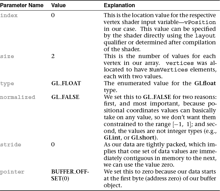
We hope that explanation of how we arrived at the parameters will help you determine the necessary values for your own data structures. We will have plenty more examples of using glVertexAttribPointer().
One additional technique we use is using our BUFFER_OFFSET macro in glVertexAttribPointer() to specify the offset. There’s nothing special about our macro; here’s its definition.
#define BUFFER_OFFSET(offset) ((void *)(offset))
While there’s a long history of OpenGL lore about why one might do this,3 we use this macro to make the point that we’re specifying an offset into a buffer object, rather than a pointer to a block of memory as glVertexAttribPointer()’s prototype would suggest.
3. In versions before 3.1, vertex-attribute data was permitted to be stored in application memory instead of GPU buffer objects, so pointers made sense in that respect.
At this point, we have one task left to do in init(), which is to enable our vertex-attribute array. We do this by calling glEnableVertexAttribArray() and passing the index of the attribute array pointer we initialized by calling glVertexAttribPointer(). Here are the full details for glEnableVertexAttribArray():
It’s important to note that the state we’ve just specified by calling glVertexAttribPointer() and glEnableVertexAttribArray() is stored in the vertex array object we bound at the start of the function. The modifications to the state in this object are implied through this binding. If we wanted to set up a vertex array object without binding it to the context, we could instead call glEnableVertexArrayAttrib(), glVertexArrayAttribFormat(), and glVertexArrayVertexBuffers(), which are the direct state access versions of these functions.
Now all that’s left is to draw something.
Our First OpenGL Drawing
With all that setup and data initialization, rendering (for the moment) will be simple. While our display() routine is only four lines long, its sequence of operations is virtually the same in all OpenGL applications. Here it is once again.
void
display(void)
{
static const float black[] = { 0.0f, 0.0f, 0.0f, 0.0f };
glClearBufferfv(GL_COLOR, 0, black);
glBindVertexArray(VAOs[Triangles]);
glDrawArrays(GL_TRIANGLES, 0, NumVertices);
}
We begin rendering by clearing our framebuffer. This is done by calling glClearBufferfv().
We discuss depth and stencil buffering, as well as an expanded discussion of color, in Chapter 4, “Color, Pixels, and Fragments.”
In this example, we clear the color buffer to black. Let’s say you always want to clear the background of the viewport to white. You would call glClearBufferfv() and pass value as a pointer to an array of four floating-point 1.0 values.
Try This
Change the values in the black variables in triangles.cpp to see the effect of changing the clear color.
Drawing with OpenGL
Our next two calls select the collection of vertices we want to draw and requests that they be rendered. We first call glBindVertexArray() to select the vertex array that we want to use as vertex data. As mentioned before, you would do this to switch between different collections of vertex data.
Next, we call glDrawArrays(), which actually sends vertex data to the OpenGL pipeline.
The glDrawArrays() function can be thought of as a shortcut to the much more complex glDrawArraysInstancedBaseInstance() function which contains several more parameters. These will be explained in “Instanced Rendering” in Chapter 3.
In our example, we request that individual triangles be rendered by setting the rendering mode to GL_TRIANGLES, starting at offset zero with respect to the buffer offset we set with glVertexAttribPointer(), and continuing for NumVertices (in our case, 6) vertices. We describe all of the rendering shapes in detail in Chapter 3.
Try This
Modify triangles.cpp to render a different type of geometric primitive, like GL_POINTS or GL_LINES. Any of the listed primitives can be used, but some of the results may not be what you expect, and for GL_PATCHES, you won’t see anything as it requires use of tessellation shaders, which we discuss in Chapter 9.
That’s it! Now we’ve drawn something. The framework code will take care of showing the results to your user.
Enabling and Disabling Operations in OpenGL
One important feature that we didn’t need to use in our first program, but will use throughout this book, is enabling and disabling modes of operation in OpenGL. Most operational features are turned on and off by the glEnable() and glDisable() commands.
You may often find, particularly if you have to write libraries that use OpenGL that will be used by other programmers, that you need to determine a feature’s state before changing for your own needs. glIsEnabled() will return if a particular capability is currently enabled.