
Chapter 4. Color, Pixels, and Fragments
Chapter Objectives
After reading this chapter, you’ll be able to do the following:
• Understand how OpenGL processes and represents the colors in your generated images.
• Identify the types of buffers available in OpenGL, and be able to clear and control writing to them.
• List the various tests and operations on fragments that occur after fragment shading.
• Use alpha blending to render translucent objects realistically.
• Use multisampling and antialiasing to remove aliasing artifacts.
• Employ occlusion queries and conditional rendering to optimize rendering.
• Retrieve rendered images and copy pixels from one place to another or one framebuffer to another.
The goal of computer graphics, generally speaking, is to determine the colors that make up an image. For OpenGL, that image is usually shown in a window on a computer screen, which itself is made up of a rectangular array of pixels, each of which can display its own color. This chapter further develops how you can use shaders in OpenGL to generate the colors of the pixels in the framebuffer. We discuss how colors set in an application directly contribute to a fragment’s color, the processing that occurs after the completion of the fragment shader, and other techniques used for improving the generated image. This chapter contains the following major sections:
• “Basic Color Theory,” which briefly describes the physics of light and how colors are represented in OpenGL.
• “Buffers and Their Uses” presents different kinds of buffers, how to clear them, when to use them, and how OpenGL operates on them.
• “Color and OpenGL” explains how OpenGL processes color in its pipeline.
• “Testing and Operating on Fragments” describes the tests and additional operations that can be applied to individual fragments after the fragment shader has completed, including alpha blending.
• “Multisampling” introduces one of OpenGL’s antialiasing techniques and describes how it modifies rasterization.
• “Per-Primitive Antialiasing” presents how blending can be used to smooth the appearance of individual primitives.
• “Reading and Copying Pixel Data” shows how to read back the result of rendering.
• “Copying Pixel Rectangles” discusses how to copy a block of pixels from one section of the framebuffer to another in OpenGL.
Basic Color Theory
In the physical world, light is composed of photons—in simplest terms, tiny particles traveling along a straight path,1 each with its own “color,” which in terms of physical quantities is represented by wavelength (or frequency).2
1. Ignoring gravitational effects, of course.
2. A photon’s frequency and wavelength are related by the equation c = νλ, where c is the speed of light (3 × 10⁸meters/second), ν is the photon’s frequency, and λ its wavelength. And for those who want to debate the wave-particle duality of light, we’re always open to that discussion over a beer.
Photons that we can see have wavelengths in the visible spectrum, which ranges from about 390 nanometers (the color violet) to 720 nanometers (the color red). The colors in between form the dominant colors of the rainbow: violet, indigo, blue, green, yellow, orange, and red.
Your eye contains light-sensitive structures called rods and cones. The rods are sensitive to light intensity, while the cones are less sensitive to the intensity of light but can distinguish between different wavelengths of light. Current understanding is that there are three types of cones, each with a sensitivity to light within a different range of wavelengths. By evaluating the responses of the three types of cones, our brain is capable of perceiving many more colors than the seven that compose the colors of the rainbow. For example, ideal white light is composed of a equal quantities of photons at all visible wavelengths. By comparison, laser light is essentially monochromatic, with all the photons having an almost identical frequency.
So what does this have to do with computer graphics and OpenGL, you may ask? Modern display devices have a much more restricted range of colors they can display, only a portion of the visible spectrum, though this is improving with time. The set of colors a device can display is often represented as its gamut. Most display devices you’ll work with while using OpenGL create their colors using a combination of three primary colors—red, green, and blue—which form the spectrum of colors that the device can display. We call that the RGB color space and use a set of three values for each color. The reason that we can use only three colors to represent such a large portion of the visible spectrum is that these three colors fall quite close to the centers of the response curves of the cones in our eyes.
In OpenGL, we often pack those three components with a fourth component alpha (which we discuss later in “Blending”), which we’ll predictably call the RGBA color space. In addition to RGB, OpenGL supports the sRGB color space. We’ll encounter sRGB when we discuss framebuffer objects and texture maps.
Note
There are many color spaces, like HSV (Hue-Saturation-Value) or CMYK (Cyan-Magenta-Yellow-Black). If your data is in a color space different from RGB, you’ll need to convert it from that space into RGB (or sRGB) to process it with OpenGL.
Unlike light in the physical world, where frequencies and intensities range continuously, computer framebuffers can represent only a comparatively small number of discrete values (although usually numbering in the millions of colors). This quantization of intensities limits the number of colors we can display. Normally, each component’s intensity is stored using a certain number of bits (usually called its bit depth), and the sum of each component’s bit depth (excluding alpha) determines the color buffer’s depth, which also determines the total number of display colors. For example, a common format for the color buffer is eight bits for each red, green, and blue. This yields a 24-bit deep color buffer, which is capable of displaying 224 unique colors. “Data in OpenGL Buffers” in Chapter 3 expanded on the types of buffers that OpenGL makes available and describes how to control interactions with those buffers.
Buffers and Their Uses
An important goal of almost every graphics program is to draw pictures on the screen (or into an off-screen buffer). The framebuffer (which is most often the screen) is composed of a rectangular array of pixels, each capable of displaying a tiny square of color at that point in the image. After the rasterization stage, which is where the fragment shader was executed, the data are not pixels yet, just fragments. Each fragment has coordinate data that corresponds to a pixel, as well as color and depth values.
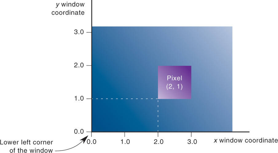
As shown in Figure 4.1, usually, the lower-left pixel in an OpenGL window is pixel (0, 0), corresponding to the window coordinates of the lower-left corner of the 1 × 1 region occupied by this pixel. In general, pixel (x, y) fills the region bounded by x on the left, x + 1 on the right, y on the bottom, and y + 1 on the top.
As an example of a buffer, let’s look more closely at the color buffer, which holds the color information that’s to be displayed on the screen. Let’s say that the screen is 1920 pixels wide and 1080 pixels high and that it’s a full 24-bit color screen. In other words, there are 224 (or 16,777,216) different colors that can be displayed. Because 24 bits translate to 3 bytes (8 bits per byte), the color buffer in this example has to store at least 3 bytes of data for each of the 2,073,600 (1920 × 1080) pixels on the screen. A particular hardware system might have more or fewer pixels on the physical screen, as well as more or less color data per pixel. Any particular color buffer, however, has the same amount of data for each pixel on the screen.
The color buffer is only one of several buffers that hold information about a pixel. In fact, a pixel may have many color buffers associated with it. The framebuffer on a system comprises all of these buffers, and you can use multiple framebuffers within your application. We’ll discuss this more in “Framebuffer Objects” in Chapter 6. With the exception of the primary color buffer, you don’t view these other buffers directly; instead, you use them to perform such tasks as hidden-surface removal, stenciling, dynamic texture generation, and other operations.
Within an OpenGL system the following types of buffers are available:
• Color buffers, of which there might be one or several active
• Depth buffer
• Stencil buffer
All of those buffers collectively form the framebuffer, although it’s up to you to decide which of those buffers you need to use. When your application starts, you’re using the default framebuffer, which is the one related to the windows of your application. The default framebuffer will always contain a color buffer.
Your particular OpenGL implementation determines which buffers are available and how many bits per pixel each buffer holds. Additionally, you can have multiple visuals, or window types, that also may have different buffers available. As we describe each of the types of buffers, we’ll also cover ways you can query their capabilities, in terms of data storage and precision.
We now briefly describe the type of data that each buffer type stores and then move to discussing operations that you do with each type of buffer.
Color Buffers
The color buffers are the ones to which you usually draw. They contain the RGB or sRGB color data and may also contain alpha values for each pixel in the framebuffer. There may be multiple color buffers in a framebuffer. The “main” color buffer of the default framebuffer is special because it’s the one associated with your window on the screen and where you will draw to have your image shown on the screen (assuming you want to display an image there). All other buffers are off screen.
The pixels in a color buffer may store a single color per pixel or may logically divide the pixel into subpixels, which enables an antialiasing technique called multisampling. We discuss multisampling in detail in “Multisampling” on page 185.
You’ve already used double buffering for animation. Double buffering is done by making the main color buffer have two parts: a front buffer that’s displayed in your window; and a back buffer, which is where you render the new image. When you swap the buffers (by calling glfwSwapBuffers(), for example), the front and back buffers are exchanged. Only the main color buffer of the default framebuffer is double buffered.
Additionally, an OpenGL implementation might support stereoscopic viewing, in which case the color buffer (even if it’s double buffered) will have left and right color buffers for the respective stereo images.
Depth Buffer
The depth buffer stores a depth value for each pixel and is used for determining the visibility of objects in a three-dimensional scene. Depth is measured in terms of distance to the eye, so pixels with larger depth-buffer values are overwritten by pixels with smaller values. This is just a useful convention, however, and the depth buffer’s behavior can be modified as described in “Depth Test” on page 170. The depth buffer is sometimes called the z-buffer (the z comes from the fact that x- and y-values measure horizontal and vertical displacement on the screen and the z-value measures distance perpendicular into the screen).
Stencil Buffer
Finally, the stencil buffer is used to restrict drawing to certain portions of the screen. Think of it like a cardboard stencil that can be used with a can of spray paint to make fairly precise painted images. For example, a classic use is to simulate the view of a rearview mirror in a car. You render the shape of the mirror to the stencil buffer, and then draw the entire scene. The stencil buffer prevents anything that wouldn’t be visible in the mirror from being drawn. We discuss the stencil buffer in “Stencil Test” on page 166.
Clearing Buffers
Probably the most common graphics activity after rendering is clearing buffers. You will probably do it once per frame (at least), and as such, OpenGL provides special functions to do this for you as optimally as possible. As you’ve seen in our examples, we set the value that each type of buffer should be initialized to in init() (if we don’t use the default values) and then clear all the buffers we need.
To clear the color buffer, call glClearBufferfv(), which was briefly introduced in Chapter 1 and whose prototype is
When you call glClearBufferfv() with the buffer argument set to GL_COLOR, one of the attached color buffers is cleared. Later, we will discuss methods to draw into multiple color buffers simultaneously. However, for now, just set drawbuffer to zero. value is a pointer to an array of four floating-point values which represent the color to which you wish to clear the color buffer, in the order red, green, blue, and alpha.
You can also clear the depth buffer with glClearBufferfv() function by setting buffer to GL_DEPTH. In this case, drawbuffer must be set to zero (because there is only ever one depth buffer) and value points to a single floating-point number, which is what the depth buffer will be cleared to.
Alternative versions of this function can be used to clear the stencil buffer (which contains integer data) or both the depth and stencil buffers at the same time. This is a common operation, and often hardware has a “fast path” for drawing to the depth and stencil buffers at the same time.
Masking Buffers
Before OpenGL writes data into the enabled color, depth, or stencil buffers, a masking operation is applied to the data, as specified with one of the following commands:
Note
The mask specified by glStencilMask() controls which stencil bitplanes are written. This mask isn’t related to the mask that’s specified as the third parameter of glStencilFunc(), which specifies which bit planes are considered by the stencil function.
Color and OpenGL
How do we use color in OpenGL? As you’ve seen, it’s the job of the fragment shader to assign a fragment’s color. There are many ways this can be done:
• The fragment shader can generate the fragment’s color without using any “external” data (i.e., data passed into the fragment shader). A very limited example of this was done in our shaders from Chapter 1 where we assigned a constant color to each fragment.
• Additional color data could be provided with each input vertex, potentially modified by another shading stage (e.g., vertex shading), and passed to the fragment shader, which uses that data to determine a color. We’ll demonstrate that in “Smoothly Interpolating Data” on page 160 in this chapter.
• Supplemental data, but not specifically colors, could be provided to the fragment shader and used in a computation that generates a color (we’ll use this technique in Chapter 7, “Light and Shadow”).
• External data, like a digital image, can be referenced in a fragment shader, which can look up colors (or other data values as well). Such data are stored in a texture map, yielding a technique called texture mapping, which we describe in Chapter 6, “Textures and Framebuffers.”
Color Representation and OpenGL
Before we analyze those techniques in depth, let’s discuss how OpenGL internally works with colors. We know that the framebuffer requires red, green, and blue values to specify a color for a pixel, so we hope it’s clear that we’ll need to provide enough information to the fragment shader to generate those values.
In the most common cases, OpenGL internally represents a color component as a floating-point value and maintains its precision until that value is stored in the framebuffer. Put another way, unless you specify otherwise, a fragment shader will receive its inputs as floating-point values, which it assigns to its fragment’s color, and those values are expected to be in the range [0.0, 1.0]—what we called a normalized value.3 That color, as it’s written into the framebuffer, will be mapped into the range of values the framebuffer can support. For instance, if the framebuffer once again has eight bits for each of red, green, and blue, the possible range for any color component is [0, 255].
3. Signed normalized values are clamped to the range [–1.0, 1.0].
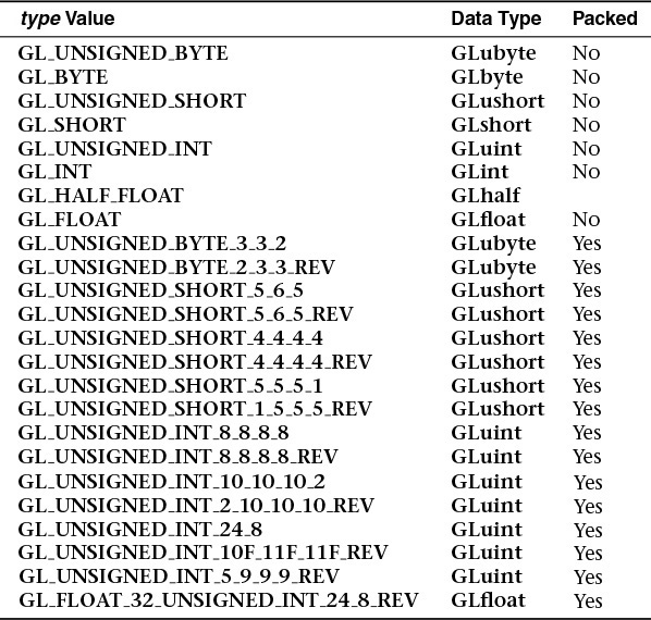
Your application can provide data into OpenGL in almost any basic C data type (e.g., int, or float). You have the choice of requesting OpenGL automatically convert non-floating-point values into normalized floating-point values. You do this with the glVertexAttribPointer() or glVertexAttribN*() routines, where OpenGL will convert the values from the input data type into the suitable normalized-value range (depending on whether the input data type was signed or unsigned). Table 4.1 describes how those data values are converted.

Smoothly Interpolating Data
Let’s take a closer look at specifying data with a vertex. Recall from Chapter 1 that vertices can have multiple data values associated with them, and colors can be among them. As with any other vertex data, the color data must be stored in a vertex-buffer object. As data is passed from the vertex shader to the fragment shader, OpenGL will smoothly interpolate it across the face of the primitive being rendered. By using this data to generate colors in the fragment shader, we can produce smooth shaded objects on the screen. This is known as Gouraud shading. In Example 4.1, we interleave the vertices’ color and position data and use an integer-valued type to illustrate having OpenGL normalize our values.
Example 4.1 Specifying Vertex Color and Position Data: gouraud.cpp
//////////////////////////////////////////////////////////////////////
//
// Gouraud.cpp
//
//////////////////////////////////////////////////////////////////////
#include <iostream>
using namespace std;
#include "vgl.h"
#include "LoadShaders.h"
enum VAO_IDs { Triangles, NumVAOs };
enum Buffer_IDs { ArrayBuffer, NumBuffers };
enum Attrib_IDs { vPosition = 0, vColor = 1 };
GLuint VAOs[NumVAOs];
GLuint Buffers[NumBuffers];
const GLuint NumVertices = 6;
//--------------------------------------------------------------------
//
// init
//
void
init(void)
{
glGenVertexArrays(NumVAOs, VAOs);
glBindVertexArray(VAOs[Triangles]);
struct VertexData {
GLubyte color[4];
GLfloat position[4];
};
VertexData vertices[NumVertices] = {
{{ 255, 0, 0, 255 }, { -0.90, -0.90 }}, // Triangle 1
{{ 0, 255, 0, 255 }, { 0.85, -0.90 }},
{{ 0, 0, 255, 255 }, { -0.90, 0.85 }},
{{ 10, 10, 10, 255 }, { 0.90, -0.85 }}, // Triangle 2
{{ 100, 100, 100, 255 }, { 0.90, 0.90 }},
{{ 255, 255, 255, 255 }, { -0.85, 0.90 }}
};
glGenBuffers(NumBuffers, Buffers);
glBindBuffer(GL_ARRAY_BUFFER, Buffers[ArrayBuffer]);
glBufferData(GL_ARRAY_BUFFER, sizeof(vertices),
vertices, GL_STATIC_DRAW);
ShaderInfo shaders[] = {
{ GL_VERTEX_SHADER, "gouraud.vert" },
{ GL_FRAGMENT_SHADER, "gouraud.frag" },
{ GL_NONE, NULL }
};
GLuint program = LoadShaders(shaders);
glUseProgram(program);
glVertexAttribPointer(vColor, 4, GL_UNSIGNED_BYTE,
GL_TRUE, sizeof(VertexData),
BUFFER_OFFSET(0));
glVertexAttribPointer(vPosition, 2, GL_FLOAT,
GL_FALSE, sizeof(VertexData),
BUFFER_OFFSET(sizeof(vertices[0].color)));
glEnableVertexAttribArray(vColor);
glEnableVertexAttribArray(vPosition);
}
Example 4.1 is only a slight modification of our example from Chapter 1, triangles.cpp. First, we created a simple structure VertexData that encapsulates all of the data for a single vertex: an RGBA color for the vertex and its spatial position. As before, we packed all the data into an array that we loaded into our vertex buffer object. As there are now two vertex attributes for our vertex data, we needed to add a second vertex attribute pointer to address the new vertex colors so we can work with that data in our shaders. For the vertex colors, we also asked OpenGL to normalize our colors by setting the fourth parameter to GL_TRUE.
To use our vertex colors, we need to modify our shaders to take the new data into account. First, let’s look at the vertex shader, which is shown in Example 4.2.
Example 4.2 A Simple Vertex Shader for Gouraud Shading
#version 330 core
layout (location = 0) in vec4 vPosition;
layout (location = 1) in vec4 vColor;
out vec4 fs_color;
void
main()
{
fs_color = vColor;
gl_Position = vPosition;
}
Modifying our vertex shader in Example 4.2 to use the new vertex colors is straightforward. We added new input and output variables: vColor, and color to complete the plumbing for getting our vertex colors into and out of our vertex shader. In this case, we simply passed through our color data for use in the fragment shader, as in Example 4.3.
Example 4.3 A Simple Fragment Shader for Gouraud Shading
#version 330 core
in vec4 fs_color;
out vec4 color;
void
main()
{
color = fs_color;
}
The fragment shader in Example 4.3, looks pretty simple as well, just assigning the shader’s input color to the fragment’s output color. However, what’s different is that the colors passed into the fragment shader don’t come directly from the immediately preceding shader stage (i.e., the vertex shader), but from the rasterizer.
Testing and Operating on Fragments
When you draw geometry on the screen, OpenGL starts processing it by executing the currently bound vertex shader; then the tessellation and geometry shaders, if they’re part of the current program object; and then assembles the final geometry into primitives that get sent to the rasterizer, which figures out which pixels in the window are affected. After OpenGL determines that an individual fragment should be generated, its fragment shader is executed, followed by several processing stages, which control how and whether the fragment is drawn as a pixel into the framebuffer, remain. For example, if the fragment is outside a rectangular region or if it’s farther from the viewpoint than the pixel that’s already in the framebuffer, its processing is stopped, and it’s not drawn. In another stage, the fragment’s color is blended with the color of the pixel already in the framebuffer.
This section describes both the complete set of tests that a fragment must pass before it goes into the framebuffer and the possible final operations that can be performed on the fragment as it’s written. Most of these tests and operations are enabled and disabled using glEnable() and glDisable(), respectively. The tests and operations occur in the following order. If a fragment is eliminated in an enabled earlier test, none of the later enabled tests or operations are executed:
1. Scissor test
2. Multisample fragment operations
3. Stencil test
5. Blending
6. Logical operations
All of these tests and operations are described in detail in the following subsections.
Note
As we’ll see in “Framebuffer Objects” in Chapter 6, we can render into multiple buffers at the same time. Many of the fragment tests and operations can be controlled on a per-buffer basis, as well as for all of the buffers collectively. In many cases, we describe both the OpenGL function that will set the operation for all buffers, as well as the routine for affecting a single buffer. In most cases, the single buffer version of a function will have an ‘i’ appended to the function’s name.
Scissor Test
The first additional test you can enable to control fragment visibility is the scissor test. The scissor box is a rectangular portion of your window that restricts all drawing to its region. You specify the scissor box using the glScissor() command and enable the test by specifying GL_SCISSOR_TEST with glEnable(). If a fragment lies inside the rectangle, it passes the scissor test.
All rendering, including clearing the window, is restricted to the scissor box if the test is enabled (as compared to the viewport, which doesn’t limit screen clears). To determine whether scissoring is enabled and to obtain the values that define the scissor rectangle, you can use GL_SCISSOR_TEST with glIsEnabled() and GL_SCISSOR_BOX with glGetIntegerv().
OpenGL actually has multiple scissor rectangles. By default, all rendering is tested against the first of these rectangles (when scissor testing is enabled) and the glScissor() function sets new values for all of them. To access the other scissor rectangles without using extensions, a geometry shader is required, and this will be explained in “Multiple Viewports and Layered Rendering” in Chapter 10.
Multisample Fragment Operations
By default, multisampling calculates fragment coverage values that are independent of alpha. However, if you glEnable() one of the following special modes, a fragment’s alpha value is taken into consideration when calculating the coverage, assuming that multisampling itself is enabled and that there is a multisample buffer associated with the framebuffer. The special modes are as follows:
• GL_SAMPLE_ALPHA_TO_COVERAGE uses the alpha value of the fragment in an implementation-dependent manner to compute the final coverage value.
• GL_SAMPLE_ALPHA_TO_ONE the sets the fragment’s alpha value to the maximum alpha value and then uses that value in the subsequent calculations. If GL_SAMPLE_ALPHA_TO_COVERAGE is also enabled, the value alpha for the fragment before substitution is used rather than the substituted value of 1.0.
• GL_SAMPLE_COVERAGE uses the value set with the glSampleCoverage() routine, which is combined (ANDed) with the calculated coverage value. Additionally, the generated sample mask can be inverted by setting the invert flag with the glSampleCoverage() routine.
• GL_SAMPLE_MASK specifies an exact bit-representation for the coverage mask (as compared to it being generated by the OpenGL implementation). This mask has one bit for each sample in the framebuffer and is once again ANDed with the sample coverage for the fragment. The sample mask is specified using the glSampleMaski() function.
The sample mask can also be specified in a fragment shader by writing to the gl_SampleMask variable, which is also an array of 32-bit words. Details of using gl_SampleMask are covered in Appendix C, “Built-in GLSL Variables and Functions.”
Stencil Test
The stencil test takes place only if there is a stencil buffer, which you need to request when your window is created. If there is no stencil buffer, the stencil test always passes. Stenciling applies a test that compares a reference value with the value stored at a pixel in the stencil buffer. Depending on the result of the test, the value in the stencil buffer can be modified. You can choose the particular comparison function used, the reference value, and the modification performed with the glStencilFunc() and glStencilOp() commands.
Note
If the GL_ARB_shader_stencil_export extension is supported, the value used for ref can be generated in and exported from your fragment shader. This allows a different reference value to be used for each fragment. To enable this feature, enable the GL_ARB_shader_stencil_export extension in your shader and then write to the gl_FragStencilRefARB built-in variable. When this variable is written in your fragment shader, the per-fragment value will be used in place of the value of ref passed to glStencilFunc() or glStencilFuncSeparate().
“With saturation” means that the stencil value will clamp to extreme values. If you try to decrement zero with saturation, the stencil value remains zero. “Without saturation” means that going outside the indicated range wraps around. If you try to decrement zero without saturation, the stencil value becomes the maximum unsigned integer value (quite large!).
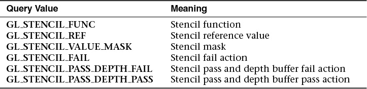
Stencil Queries
You can obtain the values for all six stencil-related parameters by using the query function glGetIntegerv() and one of the values shown in Table 4.2. You can also determine whether the stencil test is enabled by passing GL_STENCIL_TEST to glIsEnabled().
Stencil Examples
Probably the most typical use of the stencil test is to mask out an irregularly shaped region of the screen to prevent drawing from occurring within it. To do this, fill the stencil mask with zeros and then draw the desired shape in the stencil buffer with ones. You can’t draw geometry directly into the stencil buffer, but you can achieve the same result by drawing into the color buffer and choosing a suitable value for the zpass function (such as GL_REPLACE). Whenever drawing occurs, a value is also written into the stencil buffer (in this case, the reference value). To prevent the stencil-buffer drawing from affecting the contents of the color buffer, set the color mask to zero (or GL_FALSE). You might also want to disable writing into the depth buffer. After you’ve defined the stencil area, set the reference value to one, and set the comparison function such that the fragment passes if the reference value is equal to the stencil-plane value. During drawing, don’t modify the contents of the stencil planes.
Example 4.4 demonstrates how to use the stencil test in this way. Two tori are drawn, with a diamond-shaped cutout in the center of the scene. Within the diamond-shaped stencil mask, a sphere is drawn. In this example, drawing into the stencil buffer takes place only when the window is redrawn, so the color buffer is cleared after the stencil mask has been created.
Example 4.4 Using the Stencil Test: stencil.c
void
init(void)
{
... // Set up our vertex arrays and such
// Set the stencil's clear value
glClearStencil(0x0);
glEnable(GL_DEPTH_TEST);
glEnable(GL_STENCIL_TEST);
}
// Draw a sphere in a diamond-shaped section in the
// middle of a window with 2 tori.
void
display(void)
{
glClear(GL_COLOR_BUFFER_BIT | GL_DEPTH_BUFFER_BIT);
// draw sphere where the stencil is 1
glStencilFunc(GL_EQUAL, 0x1, 0x1);
glStencilOp(GL_KEEP, GL_KEEP, GL_KEEP);
drawSphere();
// draw the tori where the stencil is not 1
glStencilFunc(GL_NOTEQUAL, 0x1, 0x1);
drawTori();
}
// Whenever the window is reshaped, redefine the
// coordinate system and redraw the stencil area.
void
reshape(int width, int height)
{
glViewport(0, 0, width, height);
// create a diamond-shaped stencil area
glClear(GL_STENCIL_BUFFER_BIT);
glStencilFunc(GL_ALWAYS, 0x1, 0x1);
glStencilOp(GL_REPLACE, GL_REPLACE, GL_REPLACE);
drawMask();
}
The following examples illustrate other uses of the stencil test.
1. Capping: Suppose you’re drawing a closed convex object (or several of them, as long as they don’t intersect or enclose each other) made up of several polygons, and you have a clipping plane that may or may not slice off a piece of it. Suppose that if the plane does intersect the object, you want to cap the object with some constant-colored surface, rather than see the inside of it. To do this, clear the stencil buffer to zeros, and begin drawing with stenciling enabled and the stencil comparison function set always to accept fragments. Invert the value in the stencil planes each time a fragment is accepted. After all the objects are drawn, regions of the screen where no capping is required have zeros in the stencil planes, and regions requiring capping are nonzero. Reset the stencil function so that it draws only where the stencil value is nonzero, and draw a large polygon of the capping color across the entire screen.
2. Stippling: Suppose you want to draw an image with a stipple pattern. You can do this by writing the stipple pattern into the stencil buffer and then drawing conditionally on the contents of the stencil buffer. After the original stipple pattern is drawn, the stencil buffer isn’t altered while drawing the image, so the object is stippled by the pattern in the stencil planes.
Depth Test
For each pixel on the screen, the depth buffer keeps track of the distance between the viewpoint and the object occupying that pixel. The depth test is used to compare this stored value with that of the new fragment and deciding what to do with the result. If the specified depth test passes, the incoming depth value replaces the value already in the depth buffer.
The depth buffer is generally used for hidden-surface elimination. If a new candidate color for that pixel appears, it’s drawn only if the corresponding object is closer than the previous object. In this way, after the entire scene has been rendered, only objects that aren’t obscured by other items remain. Initially, the clearing value for the depth buffer is a value that’s as far from the viewpoint as possible, so the depth of any object is nearer than that value. If this is how you want to use the depth buffer, you simply have to enable it by passing GL_DEPTH_TEST to glEnable() and remember to clear the depth buffer before you redraw each frame. (See “Clearing Buffers” on page 156.) You can also choose a different comparison function for the depth test with glDepthFunc().
More context is provided in “OpenGL Transformations” in Chapter 5 for setting a depth range.
Polygon Offset
If you want to highlight the edges of a solid object, you might draw the object with polygon mode set to GL_FILL and then draw it again, but in a different color and with the polygon mode set to GL_LINE. However, because lines and filled polygons are not rasterized in exactly the same way, the depth values generated for the line and polygon edge are usually not the same, even between the same two vertices. The highlighting lines may fade in and out of the coincident polygons, which is sometimes called “stitching” and is visually unpleasant.
This undesirable effect can be eliminated by using polygon offset, which adds an appropriate offset to force coincident z-values apart, separating a polygon edge from its highlighting line. (The stencil buffer can also be used to eliminate stitching. However, polygon offset is almost always faster than stenciling.) Polygon offset is also useful for applying decals to surfaces by rendering images with hidden-line removal. In addition to lines and filled polygons, this technique can be used with points.
There are three different ways to turn on polygon offset, one for each type of polygon rasterization mode: GL_FILL, GL_LINE, and GL_POINT. You enable the polygon offset by passing the appropriate parameter to glEnable(): GL_POLYGON_OFFSET_FILL, GL_POLYGON_OFFSET_LINE, or GL_POLYGON_OFFSET_POINT. You must also call glPolygonMode() to set the current polygon rasterization method.
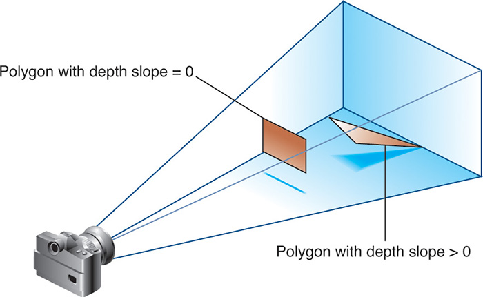
To achieve a nice rendering of the highlighted solid object without visual artifacts, you can add either a positive offset to the solid object (push it away from you) or a negative offset to the wire frame (pull it toward you). The big question is: How much offset is enough? Unfortunately, the offset required depends on various factors, including the depth slope of each polygon and the width of the lines in the wire frame.
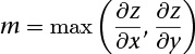
OpenGL calculates the depth slope, as illustrated in Figure 4.2, which is the z (depth) value divided by the change in either the x- or y-coordinates as you traverse the polygon. The depth values are clamped to the range [0, 1], and the x- and y-coordinates are in window coordinates. To estimate the maximum depth slope of a polygon (m in the offset equation), use this formula:

Or an implementation may use this approximation:
For polygons that are parallel to the near and far clipping planes, the depth slope is zero. Those polygons can use a small constant offset, which you can specify by setting factor to 0.0 and units to 1.0 in your call to glPolygonOffset().
For polygons that are at a great angle to the clipping planes, the depth slope can be significantly greater than zero, and a larger offset may be needed. A small, nonzero value for factor, such as 0.75 or 1.0, is probably enough to generate distinct depth values and eliminate the unpleasant visual artifacts.
In some situations, the simplest values for factor and units (1.0 and 1.0) aren’t the answer. For instance, if the widths of the lines that are highlighting the edges are greater than 1, increasing the value of factor may be necessary. Also, because depth values while using a perspective projection are unevenly transformed into window coordinates, less offset is needed for polygons that are closer to the near clipping plane, and more offset is needed for polygons that are farther away. You may need to experiment with the values you pass to glPolygonOffset() to get the result you’re looking for.
Blending
Once an incoming fragment has passed all of the enabled fragment tests, it can be combined with the current contents of the color buffer in one of several ways. The simplest way, which is also the default, is to overwrite the existing values, which admittedly isn’t much of a combination. Alternatively, you might want to combine the color present in the framebuffer with the incoming fragment color—a process called blending. Most often, blending is associated with the fragment’s alpha value (or commonly just alpha), but that’s not a strict requirement. We’ve mentioned alpha several times but haven’t given it a proper description. Alpha is the fourth color component, and all colors in OpenGL have an alpha value (even if you don’t explicitly set one). However, you don’t see alpha; rather, you see alpha’s effect: Depending on how it’s used, it can be a measure of translucency or opacity, and is what’s used when you want to simulate translucent objects, like colored glass.
However, unless you enable blending by calling glEnable() with GL_BLEND or employ advanced techniques like order-independent transparency (discussed in “Example: Order-Independent Transparency” in Chapter 11), alpha is pretty much ignored by the OpenGL pipeline. You see, just like in the real world, color of a translucent object is a combination of that object’s color with the colors of all the objects you see behind it. For OpenGL to do something useful with alpha, the pipeline needs more information than the current primitive’s color (which is the color output from the fragment shader); it needs to know what color is already present for that pixel in the framebuffer.
Blending Factors
In basic blending mode, the incoming fragment’s color is linearly combined with the current pixel’s color. As with any linear combination, coefficients control the contributions of each term. For blending in OpenGL, those coefficients are called the source- and destination-blending factors. The source-blending factor is associated with the color output from the fragment shader, and similarly, the destination-blending factor is associated with the color in the framebuffer.
If we let (Sr, Sg, Sb, Sa) represent the source-blending factors, likewise let (Dr, Dg, Db, Da) represent the destination factors, and let (Rs, Gs, Bs, As) and (Rd, Gd, Bd, Ad) represent the colors of the source fragment and destination pixel, respectively, the blending equation yields a final color of
(SrRs + DrRd, SgGs + DgGd, SbBs + DbBd, SaAs + DaAd)
The default blending operation is addition, but we’ll see in “The Blending Equation” on page 177 that we can also control the blending operator.
Controlling Blending Factors
You have two different ways to choose the source and destination blending factors. You may call glBlendFunc() and choose two blending factors: the first factor for the source RGBA and the second for the destination RGBA. Or you may use glBlendFuncSeparate() and choose four blending factors, which allows you to use one blending operation for RGB and a different one for its corresponding alpha.
Note
We also list the functions glBlendFunci() and glBlendFuncSeparatei(), which are used when you’re drawing to multiple buffers simultaneously. This is an advanced topic that we describe in “Framebuffer Objects” in Chapter 6, but because the functions are virtually identical actions to glBlendFunc() and glBlendFuncSeparate(), we include them here.
void glBlendFunc(GLenum srcfactor, GLenum destfactor);
void glBlendFunci(GLuint buffer, GLenum srcfactor,
GLenum destfactor);

In Table 4.3, the values with the subscript s1 are for dual-source blending factors, which are described in “Dual-Source Blending” on page 368.
If you use one of the GL_CONSTANT blending functions, you need to use glBlendColor() to specify the constant color.
Similarly, use glDisable() with GL_BLEND to disable blending. Note that using the constants GL_ONE (as the source factor) and GL_ZERO (for the destination factor) gives the same results as when blending is disabled; these values are the default.
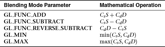
The Blending Equation
With standard blending, colors in the framebuffer are combined (using addition) with incoming fragment colors to produce the new framebuffer color. Either glBlendEquation() or glBlendEquationSeparate() may be used to select other mathematical operations to compute the difference, minimum, or maximum between color fragments and framebuffer pixels.
void glBlendEquation(GLenum mode);
void glBlendEquationi(GLuint buffer, GLenum mode);
Note
Note that as with glBlendFunci() and glBlendFuncSeparatei(), there exist glBlendEquationi() and glBlendEquationSeparatei() functions, which are also used when rendering to multiple buffers simultaneously. We cover this topic in more depth in “Framebuffer Objects” in Chapter 6.
In Table 4.4, Cs and Cd represent the source and destination colors. The S and D parameters in the table represent the source- and destination-blending factors as specified with glBlendFunc() or glBlendFuncSeparate().
Note
Note that an oddity of the GL_MIN and GL_MAX blending equations is that they do not include the source and destination factors, Srgba or Drgb, but operate only on the source and destination colors (RGBAs and RGBAd).
Logical Operations
The final operation on a fragment is the logical operation, such as an OR, XOR, or INVERT, which is applied to the incoming fragment values (source) and/or those currently in the color buffer (destination). Such fragment operations are especially useful on bit-blit-type machines, on which the primary graphics operation is copying a rectangle of data from one place in the window to another, from the window to processor memory, or from memory to the window. Typically, the copy doesn’t write the data directly into memory but allows you to perform an arbitrary logical operation on the incoming data and the data already present; then it replaces the existing data with the results of the operation.
Because this process can be implemented fairly cheaply in hardware, many such machines are available. As an examples of using a logical operation, XOR can be used to draw on an image in a revertible way; simply XOR the same drawing again, and the original image is restored.
You enable and disable logical operations by passing GL_COLOR_LOGIC_OP to glEnable() and glDisable(). You also must choose among the 16 logical operations with glLogicOp(), or you’ll just get the effect of the default value, GL_COPY.

For floating-point buffers, or those in sRGB format, logical operations are ignored.
Occlusion Query
The depth and stencil tests determine visibility on a per-fragment basis. To determine how much of a geometric object is visible, occlusion queries may be used to count the number of fragments that pass the per-fragment test.
This may be useful as a performance optimization. For complex geometric objects with many polygons, rather than rendering all of the geometry for a complex object, you might render its bounding box or another simplified representation that require less rendering resources and count the number of fragments that pass the enabled set of tests. If OpenGL returns that no fragments or samples would have been modified by rendering that piece of geometry, you know that none of your complex object will be visible for that frame, and you can skip rendering that object for the frame.
The following steps are required to utilize occlusion queries:
1. Create a query object for each occlusion query that you need with the type GL_SAMPLES_PASSED, GL_ANY_SAMPLES_PASSED, or GL_ANY_SAMPLES_PASSED_CONSERVATIVE.
2. Specify the start of an occlusion query by calling glBeginQuery().
3. Render the geometry for the occlusion test.
4. Specify that you’ve completed the occlusion query by calling glEndQuery().
5. Retrieve the number of samples, if any, that passed the depth tests.
In order to make the occlusion query process as efficient as possible, you’ll want to disable all rendering modes that will increase the rendering time but won’t change the visibility of a pixel.
Creating Query Objects
In order to use queries, you’ll first need to request identifiers for your query tests. glCreateQueries() will create the requested number of query objects for your subsequent use.
You can also determine if an identifier is currently being used as an occlusion query by calling glIsQuery().
Initiating an Occlusion Query Test
To specify geometry that’s to be used in an occlusion query, merely bracket the rendering operations between calls to glBeginQuery() and glEndQuery(), as demonstrated in Example 4.5.
Example 4.5 Rendering Geometry with Occlusion Query: occquery.c
glBeginQuery(GL_SAMPLES_PASSED, Query);
glDrawArrays(GL_TRIANGLES, 0, 3);
glEndQuery(GL_SAMPLES_PASSED);
All OpenGL operations are available while an occlusion query is active, with the exception of glCreateQueries() and glDeleteQueries(), which will raise a GL_INVALID_OPERATION error.
Note that here, we’ve introduced three occlusion query targets, all of which are related to counting samples. These are
• GL_SAMPLES_PASSED produces an exact count of the number of fragments that pass the per-fragment tests. Using this query type might reduce OpenGL performance while the query is active and should be used only if exact results are required.
• GL_ANY_SAMPLES_PASSED is also known as a Boolean occlusion query and is an approximate count. In fact, the only guarantee provided for this target is that if no fragments pass the per-fragment tests, the result of the query will be zero. Otherwise, it will be nonzero. On some implementations, the nonzero value might actually be a fairly exact count of the number of passing fragments, but you shouldn’t rely on this.
• GL_ANY_SAMPLES_PASSED_CONSERVATIVE provides an even looser guarantee than GL_ANY_SAMPLES_PASSED. For this query type, the result of the query will be zero only if OpenGL is absolutely certain that no fragments passed the test. The result might be nonzero even if no fragments made it through the tests. This may be the highest-performing of the test types but produces the least accurate results, and in practice, the performance difference is likely to be minimal. Regardless, it’s good practice to ask for only what you need, and if you don’t need the accuracy of the other test types, GL_ANY_SAMPLES_PASSED_CONSERVATIVE is a good choice.
Note
The query object mechanism is used for more than occlusion queries. Different query types are available to count vertices, primitives, and even time. These query types will be covered in the relevant sections, but use the same glBeginQuery() and glEndQuery() functions (or variations of them) that were just introduced.
Determining the Results of an Occlusion Query
Once you’ve completed rendering the geometry for the occlusion query, you need to retrieve the results. This is done with a call to glGetQueryObjectiv() or glGetQueryObjectuiv(), as shown in Example 4.6, which will return the number of fragments (or samples, if you’re using multisampling).
Example 4.6 Retrieving the Results of an Occlusion Query
count = 1000; /* counter to avoid a possible infinite loop */
do
{
glGetQueryObjectiv(Query, GL_QUERY_RESULT_AVAILABLE, &queryReady);
} while (!queryReady && count--);
if (queryReady)
{
glGetQueryObjectiv(Query, GL_QUERY_RESULT, &samples);
cerr << "Samples rendered: " << samples << endl;
}
else
{
cerr << " Result not ready ... rendering anyway" << endl;
samples = 1; /* make sure we render */
}
if (samples > 0)
{
glDrawArrays(GL_TRIANGLE_FAN}, 0, NumVertices);
}
Cleaning Up Occlusion Query Objects
After you’ve completed your occlusion query tests, you can release the resources related to those queries by calling glDeleteQueries().
Conditional Rendering
Advanced
One of the issues with occlusion queries is that they require OpenGL to pause processing geometry and fragments, count the number of affected samples in the depth buffer, and return the value to your application. Stopping modern graphics hardware in this manner usually catastrophically affects performance in performance-sensitive applications. To eliminate the need to pause OpenGL’s operation, conditional rendering allows the graphics server (hardware) to decide whether an occlusion query yielded any fragments and to render the intervening commands. Conditional rendering is enabled by surrounding the rendering operations you would have conditionally executed using the results of glGetQuery*().
The code shown in Example 4.7 replaces the sequence of code in Example 4.6. The code is not only more compact, but also far more efficient, as it removes the results query to the OpenGL server, which is a major performance inhibitor.
Example 4.7 Rendering Using Conditional Rendering
glBeginConditionalRender(Query, GL_QUERY_WAIT);
glDrawArrays(GL_TRIANGLE_FAN, 0, NumVertices);
glEndConditionalRender();
You may have noticed that there is a mode parameter to glBeginConditionalRender(), which may be one of GL_QUERY_WAIT, GL_QUERY_NO_WAIT, GL_QUERY_BY_REGION_WAIT, or GL_QUERY_BY_REGION_NO_WAIT. These modes control whether the GPU will wait for the results of a query to be ready before continuing to render and whether it will consider global results or results pertaining only to the region of the screen that contributed to the original occlusion query result.
• If mode is GL_QUERY_WAIT, the GPU will wait for the result of the occlusion query to be ready before determining whether it will continue with rendering.
• If mode is GL_QUERY_NO_WAIT, the GPU may not wait for the result of the occlusion query to be ready before continuing to render. If the result is not ready, it may choose to render the part of the scene contained in the conditional rendering section anyway.
• If mode is GL_QUERY_BY_REGION_WAIT, the GPU will wait for anything that contributes to the region covered by the controlled rendering to be completed. It may still wait for the complete occlusion query result to be ready.
• If mode is GL_QUERY_BY_REGION_NO_WAIT, the GPU will discard any rendering in regions of the framebuffer that contributed no samples to the occlusion query, but it may choose to render into other regions if the result was not available in time.
By using these modes wisely, you can improve performance of the system. For example, waiting for the results of an occlusion query may actually take more time than just rendering the conditional part of the scene. In particular, if it is expected that most results will mean that some rendering should take place, in aggregate, it may be faster to always use one of the NO_WAIT modes, even if it means more rendering will take place overall.
Multisampling
Multisampling is a technique for smoothing the edges of geometric primitives, commonly known as antialiasing. There are many ways to do antialiasing, and OpenGL supports different methods for supporting antialiasing. Other methods require some techniques we haven’t discussed yet, so we’ll defer that conversation until “Per-Primitive Antialiasing” on page 188.
Multisampling works by sampling each geometric primitive multiple times per pixel. Instead of keeping a single color (and depth and stencil values, if present) for each pixel, multisampling uses multiple samples, which are like mini-pixels, to store color, depth, and stencil values at each sample location. When it comes time to present the final image, all of the samples for the pixel are resolved to determine the final pixel’s color. Aside from a little initialization work and turning on the feature, multisampling requires very little modification to an application.
Your application begins by requesting a multisampled buffer (which is done when creating your window). You can determine whether the request was successful (as not all implementations support multisampling) by querying GL_SAMPLE_BUFFERS using glGetIntegerv(). If the value is one, multisampled rasterization can be used; if not, single-sample rasterization just like normal will be used. To engage multisampling during rendering, call glEnable() with GL_MULTISAMPLE. Because multisampling takes additional time in rendering each primitive, you may not always want to multisample all of your scene’s geometry.
Next, it’s useful to know how many samples per pixel will be used when multisampling, which you can determine by calling glGetIntegerv() with GL_SAMPLES. This value is useful if you wish to know the sample locations within a pixel, which you can find using the glGetMultisamplefv() function.
From within a fragment, you can get the same information by reading the value of gl_SamplePosition. Additionally, you can determine which sample your fragment shader is processing by using the gl_SampleID variable.
With multisampling only enabled, the fragment shader will be executed as normal, and the resulting color will be distributed to all samples for the pixels. That is, the color value will be the same, but each sample will receive individual depth and stencil values from the rasterizer. However, if your fragment shader uses either of the previously mentioned gl_Sample* variables or modifies any of its shader input variables with the sample keyword, the fragment shader will be executed multiple times for that pixel, once for each active sample location, as in Example 4.8.
Example 4.8 A Multisample-Aware Fragment Shader
#version 430 core
sample in vec4 color;
out vec4 fColor;
void main()
{
fColor = color;
}
The simple addition of the sample keyword in Example 4.8 causes each instance of the sample shader (which is the terminology used when a fragment shader is executed per sample) to receive slightly different values based on the sample’s location. Using these, particularly when sampling a texture map, will provide better results.
Sample Shading
If you can’t modify a fragment shader to use the sample keyword (e.g., you’re creating a library that accepts shaders created by another programmer), you can have OpenGL do sample shading by passing GL_SAMPLE_SHADING to glEnable(). This will cause unmodified fragment shader in variables to be interpolated to sample locations automatically.
In order to control the number of samples that receive unique sample-based interpolated values to be evaluated in a fragment shader, you can specify the minimum-sample-shading ratio with glMinSampleShading().
You might ask why specify a fraction, as compared to an absolute number of samples? Various OpenGL implementations may have differing numbers of samples per pixel. Using a fraction-based approach reduces the need to test multiple sample configurations.
Additionally, multisampling using sample shading can add a lot more work in computing the color of a pixel. If your system has four samples per pixels, you’ve quadrupled the work per pixel in rasterizing primitives, which can potentially hinder your application’s performance. glMinSampleShading() controls how many samples per pixel receive individually shaded values (i.e., each executing its own version of the bound fragment shader at the sample location). Reducing the minimum-sample-shading ratio can help improve performance in applications bound by the speed at which it can shade fragments.
As you saw in “Testing and Operating on Fragments” on page 163, a fragment’s alpha value can be modified by the results of shading at sample locations.
Per-Primitive Antialiasing
You might have noticed in some of your OpenGL images that lines, especially nearly horizontal and nearly vertical ones, appear jagged. These jaggies appear because the ideal line is approximated by a series of pixels that must lie on the pixel grid. The jaggedness is called aliasing, and this section describes one antialiasing technique for reducing it. Figure 4.3 shows two intersecting lines, both aliased and antialiased. The pictures have been magnified to show the effect.
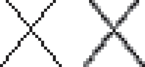
Figure 4.3 shows how a diagonal line 1 pixel wide covers more of some pixel squares than others. In fact, when performing antialiasing, OpenGL calculates a coverage value for each fragment based on the fraction of the pixel square on the screen that it would cover. OpenGL multiplies the fragment’s alpha value by its coverage. You can then use the resulting alpha value to blend the fragment with the corresponding pixel already in the framebuffer.
The details of calculating coverage values are complex and difficult to specify in general. In fact, computations may vary slightly depending on your particular implementation of OpenGL. You can use the glHint() command to exercise some control over the trade-off between image quality and speed, but not all implementations will take the hint.
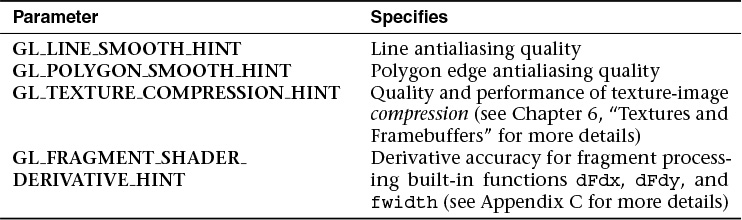
We’ve discussed multisampling before as a technique for antialiasing; however, it’s not usually the best solution for lines. Another way to antialias lines, and polygons if the multisample results are not quite what you want, is to turn on antialiasing with glEnable(), and pass in GL_LINE_SMOOTH or GL_POLYGON_SMOOTH, as appropriate. You might also want to provide a quality hint with glHint(). We describe the steps for each type of primitive that can be antialiased in the next sections.
Antialiasing Lines
First, you need to enable blending. The blending factors you most likely want to use are GL_SRC_ALPHA (source) and GL_ONE_MINUS_SRC_ALPHA (destination). Alternatively, you can use GL_ONE for the destination factor to make lines a little brighter where they intersect. Now you’re ready to draw whatever points or lines you want antialiased. The antialiased effect is most noticeable if you use a fairly high alpha value. Remember that because you’re performing blending, you might need to consider the rendering order. However, in most cases, the ordering can be ignored without significant adverse effects. Example 4.9 shows the initialization for line antialiasing.
Example 4.9 Setting Up Blending for Antialiasing Lines: antilines.cpp
glEnable (GL_LINE_SMOOTH);
glEnable (GL_BLEND);
glBlendFunc (GL_SRC_ALPHA, GL_ONE_MINUS_SRC_ALPHA);
glHint (GL_LINE_SMOOTH_HINT, GL_DONT_CARE);
Antialiasing Polygons
Antialiasing the edges of filled polygons is similar to antialiasing lines. When different polygons have overlapping edges, you need to blend the color values appropriately.
To antialias polygons, you use the alpha value to represent coverage values of polygon edges. You need to enable polygon antialiasing by passing GL_POLYGON_SMOOTH to glEnable(). This causes pixels on the edges of the polygon to be assigned fractional alpha values based on their coverage, as though they were lines being antialiased. Also, if you desire, you can supply a value for GL_POLYGON_SMOOTH_HINT.
In order to have edges blend appropriately, set the blending factors to GL_SRC_ALPHA_SATURATE (source) and GL_ONE (destination). With this specialized blending function, the final color is the sum of the destination color and the scaled source color; the scale factor is the smaller of either the incoming source alpha value or one minus the destination alpha value. This means that for a pixel with a large alpha value, successive incoming pixels have little effect on the final color because one minus the destination alpha is almost zero. With this method, a pixel on the edge of a polygon might be blended eventually with the colors from another polygon that’s drawn later. Finally, you need to sort all the polygons in your scene so that they’re ordered from front to back before drawing them.
Note
Antialiasing can be adversely affected when using the depth buffer, in that pixels may be discarded when they should have been blended. To ensure proper blending and antialiasing, you’ll need to disable the depth buffer.
Reading and Copying Pixel Data
Once your rendering is complete, you may want to retrieve the rendered image for posterity. In that case, you can use the glReadPixels() function to read pixels from the read framebuffer and return the pixels to your application. You can return the pixels into memory allocated by the application or into a pixel pack buffer, if one’s currently bound.
void glReadPixels(GLint x, GLint y, GLsizei width, GLsizei height,
GLenum format, GLenum type, void *pixels);

You may need to specify which buffer you want to retrieve pixel values from. For example, in a double-buffered window, you could read the pixels from the front buffer or the back buffer. You can use the glReadBuffer() routine to specify which buffer to retrieve the pixels from.
Clamping Returned Values
Various types of buffers within OpenGL, most notably floating-point buffers, can store values with ranges outside of the normal [0, 1] range of colors in OpenGL. When you read those values back using glReadPixels(), you can control whether the values should be clamped to the normalized range or left at their full range using glClampColor().
Copying Pixel Rectangles
To copy pixels between regions of a buffer or even different framebuffers, use glBlitNamedFramebuffer(). It uses greater pixel filtering during the copy operation, much in the same manner as texture mapping (in fact, the same filtering operations, GL_NEAREST and GL_LINEAR are used during the copy). Additionally, this routine is aware of multisampled buffers and supports copying between different framebuffers (as controlled by framebuffer objects).