
Chapter 12. Compute Shaders
Chapter Objectives
After reading this chapter, you’ll be able to do the following:
• Create, compile, and link compute shaders.
• Launch compute shaders, which operate on buffers, images, and counters.
• Allow compute shader invocations to communicate with each other and to synchronize their execution.
Compute shaders run in a completely separate stage of the GPU from the rest of the graphics pipeline. They allow an application to make use of the power of the GPU for general-purpose work that may or may not be related to graphics. Compute shaders have access to many of the same resources as graphics shaders but have more control over their application flow and how they execute. This chapter introduces the compute shader and describes its use.
This chapter has the following major sections:
• The “Overview” section introduces compute shaders and outlines their general operation.
• The organization and detailed working of compute shaders with regards to the graphics processor is given in the “Workgroups and Dispatch” section.
• Next, methods for communicating between the individual invocations of a compute shader are presented in the “Communication and Synchronization” section, along with the synchronization mechanisms that can be used to control the flow of data between those invocations.
• A few examples of compute shaders are shown, including both graphics and nongraphics work, in the “Examples” section.
• “Chapter Summary” gives concise steps for making compute shaders and suggests several best practices for using them.
Overview
The graphics processor is an immensely powerful device, capable of performing trillions of calculations each second. Over the years, it has been developed to crunch the huge amount of math operations required to render real-time graphics. However, it is possible to use the computational power of the processor for tasks that are not considered graphics or that don’t fit neatly into the relatively fixed graphical pipeline. To enable this type of use, OpenGL includes a special shader stage called the compute shader. The compute shader can be considered a special, single-stage pipeline that has no fixed input or output. Instead, all automatic input is through a handful of built-in variables. If additional input is needed, those fixed-function inputs may be used to control access to textures and buffers. All visible side effects are through image stores, atomics, and access to atomic counters. While at first this seems quite limiting, it includes general read and write of memory, and this level of flexibility and lack of graphical idioms open up a wide range of applications for compute shaders.
Compute shaders in OpenGL are very similar to any other shader stage. They are created using the glCreateShader() function, compiled using glCompileShader(), and attached to program objects using glAttachShader(). These programs are linked as normal by using glLinkProgram(). Compute shaders are written in GLSL, and in general, any functionality accessible to normal graphics shaders (for example, vertex, geometry, or fragment shaders) is available. Obviously, this excludes graphics pipeline functionality such as the geometry shaders’ EmitVertex() or EndPrimitive(), or the similarly pipeline-specific built-in variables. On the other hand, several built-in functions and variables are available to a compute shader that are available nowhere else in the OpenGL pipeline.
Workgroups and Dispatch
Just as the graphics shaders fit into the pipeline at specific points and operate on graphics-specific elements, compute shaders effectively fit into the (single-stage) compute pipeline and operate on compute-specific elements. In this analogy, vertex shaders execute per vertex, geometry shaders execute per primitive, and fragment shaders execute per fragment. Performance of graphics hardware is obtained through parallelism, which in turn is achieved through the very large number of vertices, primitives, or fragments, respectively, passing through each stage of the pipeline. In the context of compute shaders, this parallelism is more explicit, with work being launched in groups known as workgroups. Workgroups have a local neighborhood known as a local workgroup, and these are again grouped to form a global workgroup as the result of one of the dispatch commands.
The compute shader is then executed once for each element of each local workgroup within the global workgroup. Each element of the workgroup is known as a work item and is processed by an invocation. The invocations of the compute shader can communicate with each other via variables and memory and can perform synchronization operations to keep their work coherent. Figure 12.1 shows a schematic of this work layout. In this simplified example, the global workgroup consists of 16 local workgroups, and each local workgroup consists of 16 invocations, arranged in a 4 × 4 grid. Each invocation has a local index that is a two-dimensional vector.

While Figure 12.1 visualizes the global and local workgroups as two-dimensional entities, they are in fact three-dimensional. To issue work that is logically one- or two-dimensional, we simply make a three-dimensional work size where the extent in one or two of the dimensions is of size one. The invocations of a compute shader are essentially independent and may run in parallel on some implementations of OpenGL. In practice, most OpenGL implementations will group subsets of the work together and run it in lockstep, grouping yet more of these subsets together to form the local workgroups. The size of a local workgroup is defined in the compute shader source code using an input layout qualifier. The global workgroup size is measured as an integer multiple of the local workgroup size. As the compute shader executes, it is provided with its location within the local workgroup, the size of the workgroup, and the location of its local workgroup within the global workgroup through built-in variables. There are further variables available that are derived from these, providing the location of the invocation within the global workgroup, among other things. The shader may use these variables to determine which elements of the computation it should work on and also can know its neighbors within the workgroup, which facilitates some amount of data sharing.
The input layout qualifiers that are used in the compute shader to declare the local workgroup size are local_size_x, local_size_y, and local_size_z. The defaults for these are all one, so omitting local_size_z, for example, would create an N × M two-dimensional workgroup size. An example of declaring a shader with a local workgroup size of 16 × 16 is shown in Example 12.1.
Example 12.1 Simple Local Workgroup Declaration
#version 430 core
// Input layout qualifier declaring a 16 x 16 (x 1) local
// workgroup size
layout (local_size_x = 16, local_size_y = 16) in;
void main(void)
{
// Do nothing.
}
Although the simple shader of Example 12.1 does nothing, it is a valid compute shader and will compile, link, and execute on an OpenGL implementation. To create a compute shader, simply call glCreateShader() with type set to GL_COMPUTE_SHADER, set the shader’s source code with glShaderSource() and compile it as normal. Then attach the shader to a program and call glLinkProgram(). This creates the executable for the compute shader stage that will operate on the work items. A complete example of creating and linking a compute program1 is shown in Example 12.2.
1. We use the term compute program to refer to a linked program object containing a compute shader.
Example 12.2 Creating, Compiling, and Linking a Compute Shader
GLuint shader, program;
static const GLchar* source[] =
{
"#version 430 core
"
"
"
"// Input layout qualifier declaring a 16 x 16 (x 1) local
"
"// workgroup size
"
"layout (local_size_x = 16, local_size_y = 16) in;
"
"
"
"void main(void)
"
"{
"
" // Do nothing.
"
"}
"
};
shader = glCreateShader(GL_COMPUTE_SHADER);
glShaderSource(shader, 1, source, NULL);
glCompileShader(shader);
program = glCreateProgram();
glAttachShader(program, shader);
glLinkProgram(program);
Once we have created and linked a compute shader as shown in Example 12.2, we can make the program current using glUseProgram() and then dispatch workgroups into the compute pipeline using the function glDispatchCompute(), whose prototype is as follows:
When you call glDispatchCompute(), OpenGL will create a three-dimensional array of local workgroups whose size is num groups x by num_groups_y by num_groups_z groups. Remember, the size of the workgroup in one or more of these dimensions may be one, as may be any of the parameters to glDispatchCompute(). Thus, the total number of invocations of the compute shader will be the size of this array times the size of the local workgroup declared in the shader code. As you can see, this can produce an extremely large amount of work for the graphics processor, and it is relatively easy to achieve parallelism using compute shaders.
As glDrawArraysIndirect() is to glDrawArrays(), so glDispatchComputeIndirect() is to glDispatchCompute(). glDispatchComputeIndirect() launches compute work using parameters stored in a buffer object. The buffer object is bound to the GL_DISPATCH_INDIRECT_BUFFER binding point, and the parameters stored in the buffer consist of three unsigned integers, tightly packed together. Those three unsigned integers are equivalent to the parameters to glDispatchCompute(). The prototype for glDispatchComputeIndirect() is as follows:
The data in the buffer bound to GL_DISPATCH_INDIRECT_BUFFER binding could come from anywhere, including another compute shader. As such, the graphics processor can be made to feed work to itself by writing the parameters for a dispatch (or draws) into a buffer object. Example 12.3 shows an example of dispatching compute workloads using glDispatchComputeIndirect().
Example 12.3 Dispatching Compute Workloads
// program is a successfully linked program object containing a
// compute shader executable
GLuint program = ...;
// Activate the program object
glUseProgram(program);
// Create a buffer, bind it to the DISPATCH_INDIRECT_BUFFER binding
// point, and fill it with some data.
glGenBuffers(1, &dispatch_buffer);
glBindBuffer(GL_DISPATCH_INDIRECT_BUFFER, dispatch_buffer);
static const struct
{
GLuint num_groups_x;
GLuint num_groups_y;
GLuint num_groups_z;
} dispatch_params = { 16, 16, 1 };
glBufferData(GL_DISPATCH_INDIRECT_BUFFER,
sizeof(dispatch_params),
&dispatch_params,
GL_STATIC_DRAW);
// Dispatch the compute shader using the parameters stored
// in the buffer object
glDispatchComputeIndirect(0);
Notice how in Example 12.3, we simply use glUseProgram() to set the current program object to the compute program. Aside from having no access to the fixed-function graphics pipeline (such as the rasterizer or framebuffer), compute shaders and the programs that they are linked into are completely normal, first-class shader and program objects. This means that you can use glGetProgramiv() to query their properties (such as active uniform or storage blocks) and can access uniforms as normal. Of course, compute shaders also have access to almost all of the resources that other types shaders have, including images, samplers, buffers, atomic counters, and uniform blocks.
Compute shaders and their linked programs also have several compute-specific properties. For example, to retrieve the local workgroup size of a compute shader (which would have been set using a layout qualifier in the source of the compute shader), call glGetProgramiv() with pname set to GL_MAX_COMPUTE_WORK_GROUP_SIZE and param set to the address of an array of three unsigned integers. The three elements of the array will be filled with the size of the local workgroup size in the x, y, and z dimensions, in that order.
Knowing Where You Are
Once your compute shader is executing, it likely has the responsibility to set the value of one or more elements of some output array (such as an image or an array of atomic counters) or to read data from a specific location in an input array. To do this, you will need to know where in the local workgroup you are and where that workgroup is within the larger global workgroup. For these purposes, OpenGL provides several built-in variables to compute shaders. These built-in variables are implicitly declared as shown in Example 12.4.
Example 12.4 Declaration of Compute Shader Built-In Variables
const uvec3 gl_WorkGroupSize;
in uvec3 gl_NumWorkGroups;
in uvec3 gl_LocalInvocationID;
in uvec3 gl_WorkGroupID;
in uvec3 gl_GlobalInvocationID;
in uint gl_LocalInvocationIndex;
The compute shader built-in variables have the following definitions:
• gl_WorkGroupSize is a constant that stores the size of the local workgroup as declared by the local_size_x, local_size_y, and local_size_z layout qualifiers in the shader. Replicating this information here serves two purposes. First, it allows the workgroup size to be referred to multiple times in the shader without relying on the preprocessor. Second, it allows multidimensional workgroup size to be treated as a vector without having to construct it explicitly.
• gl_NumWorkGroups is a vector that contains the parameters that were passed to glDispatchCompute() (num groups x, num groups y, and num groups z). This allows the shader to know the extent of the global workgroup that it is part of. Besides being more convenient than needing to set the values of uniforms by hand, some OpenGL implementations may have a very efficient path for setting these constants.
• gl_LocalInvocationID is the location of the current invocation of a compute shader within the local workgroup. It will range from uvec3(0) to gl_WorkGroupSize - uvec3 (1).
• gl_WorkGroupID is the location of the current local workgroup within the larger global workgroup. This variable will range from uvec3(0) to gl_NumWorkGroups - uvec3 (1).
• gl_GlobalInvocationID is derived from gl_LocalInvocationID, gl_WorkGroupSize, and gl_WorkGroupID. Its exact value is equal to gl_WorkGroupID * gl_WorkGroupSize + gl_LocalInvocationID, and as such, it is effectively the three-dimensional index of the current invocation within the global workgroup.
• gl_LocalInvocationIndex is a flattened form of gl_LocalInvocationID. It is equal to gl_LocalInvocationID.z * gl_WorkGroupSize.x * gl_WorkGroupSize.y + gl_LocalInvocationID.y * gl_WorkGroupSize.x + gl_LocalInvocationID.x. It can be used to index into one-dimensional arrays that represent two- or three-dimensional data.
Given that we now know where we are within both the local workgroup and the global workgroup, we can use this information to operate on data. Taking the example of Example 12.5 and adding an image variable allows us to write into the image at a location derived from the coordinate of the invocation within the global workgroup and update it from our compute shader. This modified shader is shown in Example 12.5.
Example 12.5 Operating on Data
#version 430 core
layout (local_size_x = 32, local_size_y = 16) in;
// An image to store data into.
layout (rg32f) uniform image2D data;
void main(void)
{
// Store the local invocation ID into the image.
imageStore(data,
ivec2(gl_GlobalInvocationID.xy),
vec4(vec2(gl_LocalInvocationID.xy) /
vec2(gl_WorkGroupSize.xy),
0.0, 0.0));
}
The shader shown in Example 12.5 simply takes the local invocation index, normalizes it to the local workgroup size, and stores the result into the data image at the location given by the global invocation ID. The resulting image shows the relationship between the global and local invocation IDs and clearly shows the rectangular local workgroup size specified in the compute shader (in this case, 32 by 16 work items). The resulting image is shown in Figure 12.2.

To generate the image of Figure 12.2, after being written by the compute shader, the texture is simply rendered to a full-screen triangle fan.
Communication and Synchronization
When you call glDispatchCompute() (or glDispatchComputeIndirect()), a potentially huge amount of work is sent to the graphics processor. The graphics processor will run that work in parallel if it can, and the invocations that execute the compute shader can be considered to be a team trying to accomplish a task. Teamwork is facilitated greatly by communication, so, while the order of execution and level of parallelism is not defined by OpenGL, some level of cooperation between the invocations is enabled by allowing them to communicate via shared variables. Furthermore, it is possible to sync up all the invocations in the local workgroup so that they reach the same part of your shader at the same time.
Communication
The shared keyword is used to declare variables in shaders in a similar manner to other keywords, such as uniform, in, and out. Some example declarations using the shared keyword are shown in Example 12.6.
Example 12.6 Example of Shared Variable Declarations
// A single shared unsigned integer;
shared uint foo;
// A shared array of vectors
shared vec4 bar[128];
// A shared block of data
shared struct baz_struct
{
vec4 a_vector;
int an_integer;
ivec2 an_array_of_integers[27];
} baz[42];
When a variable is declared as shared, that means it will be kept in storage that is visible to all of the compute shader invocations in the same local workgroup. When one invocation of the compute shader writes to a shared variable, the data it wrote will eventually become visible to other invocations of that shader within the same local workgroup. We say eventually because the relative order of execution of compute shader invocations is not defined—even within the same local workgroup. Therefore, one shader invocation may write to a shared variable long before another invocation reads from that variable or even long after the other invocation has read from that variable. To ensure that you get the results you expect, you need to include some synchronization primitives in your code. These are covered in detail in the next section.
The performance of accesses to shared variables is often significantly better than accesses to images or to shader storage buffers (i.e., main memory). As shared memory is local to a shader processor and may be duplicated throughout the device, access to shared variables can be even faster than hitting the cache. For this reason, it is recommended that if your shader performs more than a few accesses to a region of memory, and especially if multiple shader invocations will access the same memory locations, that you first copy that memory into some shared variables in the shader, operate on them there, and then write the results back into main memory if required.
Because it is expected that variables declared as shared will be stored inside the graphics processor in dedicated high-performance resources, and because those resources may be limited, it is possible to query the combined maximum size of all shared variables that can be accessed by a single compute program. To retrieve this limit, call glGetIntegerv() with pname set to GL_MAX_COMPUTE_SHARED_MEMORY_SIZE.
Synchronization
If the order of execution of the invocations of a local workgroup and all of the local workgroups that make up the global workgroup are not defined, the operations that an invocation performs can occur out of order with respect to other invocations. If no communication between the invocations is required, and they can all run completely independently, this likely isn’t going to be an issue. However, if the invocations need to communicate with each other, either through images and buffers or through shared variables, it may be necessary to synchronize their operations.
There are two types of synchronization commands. The first is an execution barrier, which is invoked using the barrier() function. This is similar to the barrier() function you can use in a tessellation control shader to synchronize the invocations that are processing the control points. When an invocation of a compute shader reaches a call to barrier(), it will stop executing and wait for all other invocations within the same local workgroup to catch up. Once the invocation resumes executing, having returned from the call to barrier(), it is safe to assume that all other invocations have also reached their corresponding call to barrier() and have completed any operations that they performed before this call. The usage of barrier() in a compute shader is somewhat more flexible than what is allowed in a tessellation control shader. In particular, there is no requirement that barrier() be called only from the shader’s main() function. Calls to barrier() must, however, be executed only inside uniform flow control. That is, if one invocation within a local workgroup executes a barrier() function, all invocations within that workgroup must also execute the same call. This seems logical, as one invocation of the shader has no knowledge of the control flow of any other and must assume that the other invocations will eventually reach the barrier. If they do not, deadlock can occur.
When communicating between invocations within a local workgroup, you can write to shared variables from one invocation and then read from them in another. However, you need to make sure that by the time you read from a shared variable in the destination invocation that the source invocation has completed the corresponding write to that variable. To ensure this, you can write to the variable in the source invocation and then in both invocations execute the barrier() function. When the destination invocation returns from the barrier() call, it can be sure that the source invocation has also executed the function (and therefore completed the write to the shared variable), so it is safe to read from the variable.
The second type of synchronization primitive is the memory barrier. The heaviest, most brute-force version of the memory barrier is memoryBarrier(). When memoryBarrier() is called, it ensures that any writes to memory that have been performed by the shader invocation have been committed to memory rather than lingering in caches or being scheduled after the call to memoryBarrier(), for example. Any operations that occur after the call to memoryBarrier() will see the results of those memory writes if the same memory locations are read again, even in different invocations of the same compute shader. Furthermore, memoryBarrier() can serve as instruction to the shader compiler to not reorder memory operations if it means that they will cross the barrier. If memoryBarrier() seems somewhat heavy-handed, that would be an astute observation. In fact, there are several other memory barrier functions that serve as subsets of the memoryBarrier() mega function. In fact, memoryBarrier() is simply defined as calling each of these subfunctions back to back in some undefined (but not really relevant) order.
The memoryBarrierAtomicCounter() function wait for any updates to atomic counters to complete before continuing. The memoryBarrierBuffer() and memoryBarrierImage() functions waits for any write accesses to buffer and image variables to complete, respectively. The memoryBarrierShared() function waits for any updates to variables declared with the shared qualifier. These functions allow much finer-grained control over what types of memory accesses are waited for. For example, if you are using an atomic counter to arbitrate accesses to a buffer variable, you might want to ensure that updates to atomic counters are seen by other invocations of the shader without necessarily waiting for any prior writes to the buffer to complete, as the latter may take much longer than the former. Also, calling memoryBarrierAtomicCounter() will allow the shader compiler to reorder accesses to buffer variables without violating the logic implied by atomic counter operations.
Note that even after a call to memoryBarrier() or one of its subfunctions, there is still no guarantee that all other invocations have reached this point in the shader. To ensure this, you will need to call the execution barrier function, barrier(), before reading from memory that would have been written prior to the call to memoryBarrier().
Use of memory barriers is not necessary to ensure the observed order of memory transactions within a single shader invocation. Reading the value of a variable in a particular invocation of a shader will always return the value most recently written to that variable, even if the compiler reordered them behind the scenes.
One final function, groupMemoryBarrier(), is effectively equivalent to memoryBarrier(), except that it applies only to other invocations within the same local workgroup. All of the other memory barrier functions apply globally. That is, they ensure that memory writes performed by any invocation in the global workgroup are committed before continuing.
Examples
This section includes a number of example use cases for compute shaders. As compute shaders are designed to execute arbitrary work with very little fixed-function plumbing to tie them to specific functionality, they are very flexible and very powerful. As such, the best way to see them in action is to work through a few examples in order to see their application in real-world scenarios.
Physical Simulation
The first example is a simple particle simulator. In this example, we use a compute shader to update the positions of close to a million particles in real time. Although the physical simulation is simple, it produces visually interesting results and demonstrates the relative ease with which this type of algorithm can be implemented in a compute shader.
The algorithm implemented in this example is as follows. Two large buffers are allocated, one which stores the current velocity of each particle and a second which stores the current position. At each time step, a compute shader executes, and each invocation processes a single particle. The current velocity and position are read from their respective buffers. A new velocity is calculated for the particle, and this velocity is used to update the particle’s position. The new velocity and position are then written back into the buffers. To make the buffers accessible to the shader, they are attached to buffer textures that are then used with image load and store operations. An alternative to buffer textures is to use shader storage buffers, declared with as a buffer interface block.
In this toy example, we don’t consider the interaction of the particles with each other, which would be an O(n2) problem. Instead, we use a small number of attractors, each with a position and a mass. The mass of each particle is also considered to be the same. Each particle is considered to be gravitationally attracted to the attractors. The force exerted on the particle by each of the attractors is used to update the velocity of the particle by integrating over time. The positions and masses of the attractors are stored in a uniform block.
In addition to a position and velocity, the particles have a life expectancy. The life expectancy of the particle is stored in the w component of its position vector, and each time the particle’s position is updated, its life expectancy is reduced slightly. Once its life expectancy is below a small threshold, it is reset to one, and rather than update the particle’s position, we reset it to be close to the origin. We also reduce the particle’s velocity by two orders of magnitude. This causes aged particles (including those that may have been flung to the corners of the universe) to reappear at the center, creating a stream of fresh young particles to keep our simulation going.
The source code for the particle simulation shader is given in Example 12.7.
Example 12.7 Particle Simulation Compute Shader
#version 430 core
// Uniform block containing positions and masses of the attractors
layout (std140, binding = 0) uniform attractor_block
{
vec4 attractor[64]; // xyz = position, w = mass
};
// Process particles in blocks of 128
layout (local_size_x = 128) in;
// Buffers containing the positions and velocities of the particles
layout (rgba32f, binding = 0) uniform imageBuffer velocity_buffer;
layout (rgba32f, binding = 1) uniform imageBuffer position_buffer;
// Delta time
uniform float dt;
void main(void)
{
// Read the current position and velocity from the buffers
vec4 vel = imageLoad(velocity_buffer, int(gl_GlobalInvocationID.x));
vec4 pos = imageLoad(position_buffer, int(gl_GlobalInvocationID.x));
int i;
// Update position using current velocity * time
pos.xyz += vel.xyz * dt;
// Update 'life' of particle in w component
pos.w -= 0.0001 * dt;
// For each attractor...
for (i = 0; i < 4; i++)
{
// Calculate force and update velocity accordingly
vec3 dist = (attractor[i].xyz - pos.xyz);
vel.xyz += dt * dt *
attractor[i].w *
normalize(dist) / (dot(dist, dist) + 10.0);
}
// If the particle expires, reset it
if (pos.w <= 0.0)
{
pos.xyz = -pos.xyz * 0.01;
vel.xyz *= 0.01;
pos.w += 1.0f;
}
// Store the new position and velocity back into the buffers
imageStore(position_buffer, int(gl_GlobalInvocationID.x), pos);
imageStore(velocity_buffer, int(gl_GlobalInvocationID.x), vel);
}
To kick off the simulation, we first create the two buffer objects that will store the positions and velocities of all of the particles. The position of each particle is set to a random location in the vicinity of the origin, and its life expectancy is set to random value between zero and one. This means that each particle will reach the end of its first iteration and be brought back to the origin after a random amount of time. The velocity of each particle is also initialized to a random vector with a small magnitude. The code to do this is shown in Example 12.8.
Example 12.8 Initializing Buffers for Particle Simulation
// Generate two buffers, bind them, and initialize their data stores
glGenBuffers(2, buffers);
glBindBuffer(GL_ARRAY_BUFFER, position_buffer);
glBufferData(GL_ARRAY_BUFFER,
PARTICLE_COUNT * sizeof(vmath::vec4),
NULL,
GL_DYNAMIC_COPY);
// Map the position buffer and fill it with random vectors
vmath::vec4 * positions = (vmath::vec4 *)
glMapNamedBufferRange(position_buffer,
0,
PARTICLE_COUNT * sizeof(vmath::vec4),
GL_MAP_WRITE_BIT |
GL_MAP_INVALIDATE_BUFFER_BIT);
for (i = 0; i < PARTICLE_COUNT; i++)
{
positions[i] = vmath::vec4(random_vector(-10.0f, 10.0f),
random_float());
}
glUnmapNamedBuffer(position_buffer);
// Initialization of the velocity buffer - filled with random vectors
glBindBuffer(GL_ARRAY_BUFFER, velocity_buffer);
glBufferData(GL_ARRAY_BUFFER,
PARTICLE_COUNT * sizeof(vmath::vec4),
NULL,
GL_DYNAMIC_COPY);
vmath::vec4 * velocities = (vmath::vec4 *)
glMapBufferRange(GL_ARRAY_BUFFER,
0,
PARTICLE_COUNT * sizeof(vmath::vec4),
GL_MAP_WRITE_BIT |
GL_MAP_INVALIDATE_BUFFER_BIT);
for (i = 0; i < PARTICLE_COUNT; i++)
{
velocities[i] = vmath::vec4(random_vector(-0.1f, 0.1f), 0.0f);
}
glUnmapBuffer(GL_ARRAY_BUFFER);
The masses of the attractors are also set to random numbers between 0.5 and 1.0. Their positions are initialized to zero, but these will be moved during the rendering loop. Their masses are stored in a variable in the application because, as they are fixed, they need to be restored after each update of the uniform buffer containing the updated positions of the attractors. Finally, the position buffer is attached to a vertex array object so that the particles can be rendered as points.
The rendering loop is quite simple. First, we execute the compute shader with sufficient invocations to update all of the particles. Then we render all of the particles as points with a single call to glDrawArrays(). The shader vertex shader simply transforms the incoming vertex position by a perspective transformation matrix, and the fragment shader outputs solid white. The result of rendering the particle system as simple white points is shown in Figure 12.3.
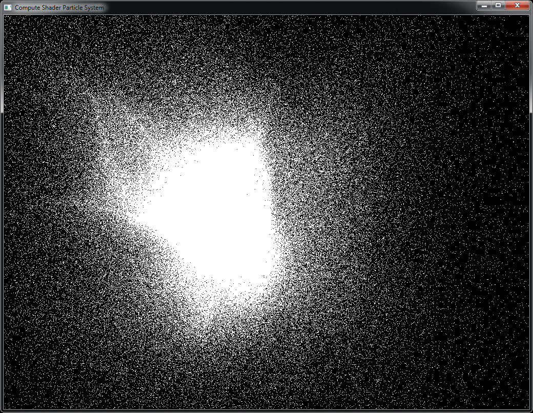
The initial output of the program is not terribly exciting. While it does demonstrate that the particle simulation is working, the visual complexity of the scene isn’t high. To add some interest to the output (this is a graphics API after all), we add some simple shading to the points.
In the fragment shader for rendering the points, we first use the age of the point (which is stored in its w component) to fade the point from red hot to cool blue as it gets older. Also, we turn on additive blending by enabling GL_BLEND and setting both the source and destination factors to GL_ONE. This causes the points to accumulate in the framebuffer and more densely populated areas to “glow” due to the number of particles in the region. The fragment shader used to do this is shown in Example 12.9.
Example 12.9 Particle Simulation Fragment Shader
#version 430 core
layout (location = 0) out vec4 color;
// This is derived from the age of the particle read
// by the vertex shader
in float intensity;
void main(void)
{
// Blend between red-hot and cool-blue based on the
// age of the particle.
color = mix(vec4(0.0f, 0.2f, 1.0f, 1.0f),
vec4(0.2f, 0.05f, 0.0f, 1.0f),
intensity);
}
In our rendering loop, the positions and masses of the attractors are updated before we dispatch the compute shader over the buffers containing the positions and velocities. We then render the particles as points having issued a memory barrier to ensure that the writes performed by the compute shader have been completed. This loop is shown in Example 12.10.
Example 12.10 Particle Simulation Rendering Loop
// Update the buffer containing the attractor positions and masses
vmath::vec4 * attractors =
(vmath::vec4 *)glMapNamedBufferRange(attractor_buffer,
0,
32 * sizeof(vmath::vec4),
GL_MAP_WRITE_BIT |
GL_MAP_INVALIDATE_BUFFER_BIT);
int i;
for (i = 0; i < 32; i++)
{
attractors[i] =
vmath::vec4(sinf(time * (float)(i + 4) * 7.5f * 20.0f) * 50.0f,
cosf(time * (float)(i + 7) * 3.9f * 20.0f) * 50.0f,
sinf(time * (float)(i + 3) * 5.3f * 20.0f) *
cosf(time * (float)(i + 5) * 9.1f) * 100.0f,
attractor_masses[i]);
}
glUnmapNamedBuffer(attractor_buffer);
// Activate the compute program and bind the position
// and velocity buffers
glUseProgram(compute_prog);
glBindImageTexture(0, velocity_tbo, 0,
GL_FALSE, 0,
GL_READ_WRITE, GL_RGBA32F);
glBindImageTexture(1, position_tbo, 0,
GL_FALSE, 0,
GL_READ_WRITE, GL_RGBA32F);
// Set delta time
glUniform1f(dt_location, delta_time);
// Dispatch the compute shader
glDispatchCompute(PARTICLE_GROUP_COUNT, 1, 1);
// Ensure that writes by the compute shader have completed
glMemoryBarrier(GL_SHADER_IMAGE_ACCESS_BARRIER_BIT);
// Set up our mvp matrix for viewing
vmath::mat4 mvp = vmath::perspective(45.0f, aspect_ratio,
0.1f, 1000.0f) *
vmath::translate(0.0f, 0.0f, -60.0f) *
vmath::rotate(time * 1000.0f,
vmath::vec3(0.0f, 1.0f, 0.0f));
// Clear, select the rendering program and draw a full-screen quad
glClear(GL_COLOR_BUFFER_BIT | GL_DEPTH_BUFFER_BIT);
glUseProgram(render_prog);
glUniformMatrix4fv(0, 1, GL_FALSE, mvp);
glBindVertexArray(render_vao);
glEnable(GL_BLEND);
glBlendFunc(GL_ONE, GL_ONE);
glDrawArrays(GL_POINTS, 0, PARTICLE_COUNT);
Finally, the result of rendering the particle system with the fragment shader of Example 12.9 and with blending turned on is shown in Figure 12.4.
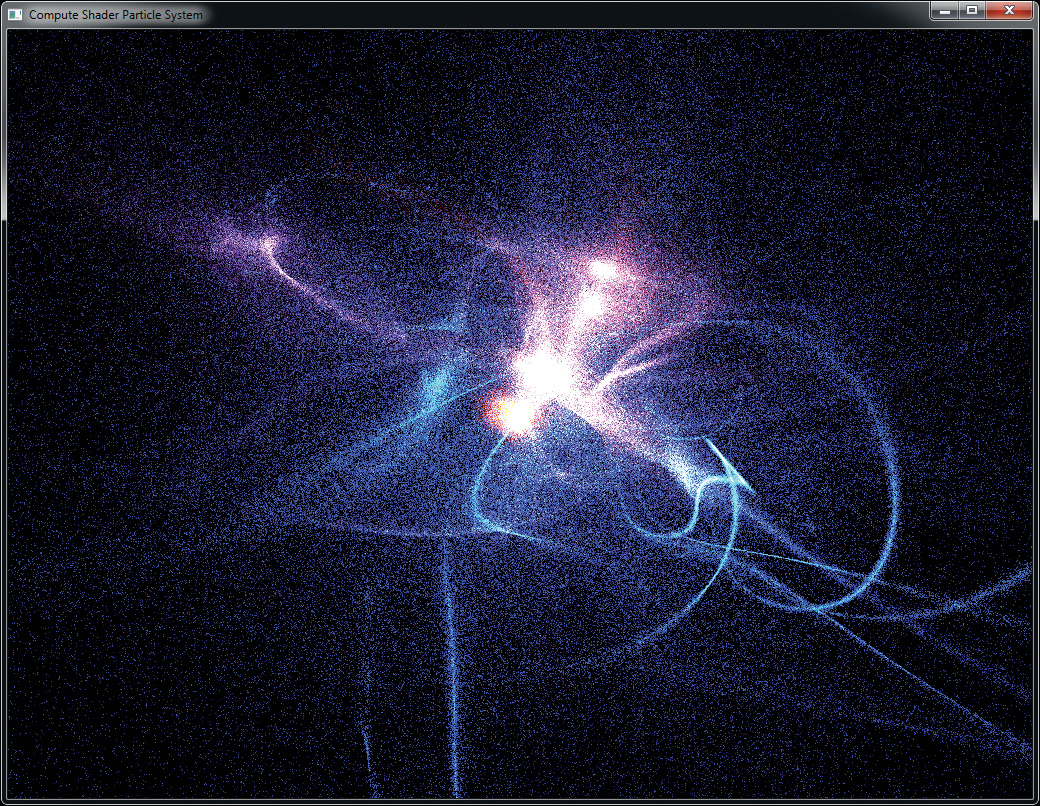
Image Processing
This example of compute shaders uses them as a means to implement image processing algorithms. In this case, we implement a simple edge-detection algorithm by convolving an input image with an edge-detection filter. The filter chosen is an example of a separable filter. A separable filter is one that can be applied one dimension at a time in a multidimensional space to produce a final result. Here, it is is applied to a two-dimensional image by applying it first in the horizontal dimension and then again in the vertical dimension. The actual kernel is a central difference kernel [–1 0 1].
To implement this kernel, each invocation of the compute shader produces a single pixel in the output image. It must read from the input image and subtract the samples to either side of the target pixel. Of course, this means that each invocation of the shader must read from the input image twice and that two invocations of the shader will read from the same location. To reduce memory accesses, this implementation uses shared variables to store a row of the input image.
Rather than reading the needed input samples directly from the input image, each invocation reads the value of its target pixel from the input image and stores it in an element of a shared array. After all invocations of the shader have read from the input image, the shared array contains a complete copy of the current scan line of the input image, each pixel of that image having been read only once. However, now that the pixels are stored in the shared array, all other invocations in the local workgroup can read from that array to retrieve the pixel values they need at very high speed.
The edge-detection compute shader is shown in Example 12.11.
Example 12.11 Central Difference Edge-Detection Compute Shader
#version 430 core
// One scan line of the image... 1024 is the minimum maximum
// guaranteed by OpenGL
layout (local_size_x = 1024) in;
// Input and output images
layout (rgba32f, binding = 0) uniform image2D input_image;
layout (rgba32f, binding = 1) uniform image2D output_image;
// Shared memory for the scanline data -- must be the same size as
// (or larger than) as the local workgroup
shared vec4 scanline[1024];
void main(void)
{
// Get the current position in the image.
ivec2 pos = ivec2(gl_GlobalInvocationID.xy);
// Read an input pixel and store it in the shared array
scanline[pos.x] = imageLoad(input_image, pos);
// Ensure that all other invocations have reached this point
// and written their shared data by calling barrier()
barrier();
// Compute our result and write it back to the image
vec4 result = scanline[min(pos.x + 1, 1023)] -
scanline[max(pos.x - 1, 0)];
imageStore(output_image, pos.yx, result);
}
The image processing shader of Example 12.11 uses a one-dimensional local workgroup size of 1024 pixels (which is the largest workgroup size that is guaranteed to be supported by an OpenGL implementation). This places an upper bound on the width or height of the image of 1024 pixels. While this is sufficient for this rather simple example, a more complex approach would be required to implement larger filters or operate on larger images.
The global invocation ID is converted to a signed integer vector and is used to read from the input image. The result is written into the scanline shared variable. Then the shader calls barrier(). This is to ensure that all of the invocations in the local workgroup have reached this point in the shader. Next, the shader takes the difference between the pixels to the left and the right of the target pixel. These values have been placed into the shared array by the invocations logically to the left and right of the current invocation. The resulting difference is placed into the output image.
Another thing to note about this shader is that when it stores the resulting pixel, it transposes the coordinates of the output pixel, effectively writing in a vertical line down the image. This has the effect of transposing the image. An alternative is to read from the input image in vertical strips and write horizontally. The idea behind this is that the same shader can be used for both passes of the separable filter, the second pass retransposing the already-transposed intermediate image, restoring it to its original orientation.
The code to invoke the compute shader is shown in Example 12.12.
Example 12.12 Dispatching the Image Processing Compute Shader
// Activate the compute program...
glUseProgram(compute_prog);
// Bind the source image as input and the intermediate
// image as output
glBindImageTexture(0, input_image, 0,
GL_FALSE, 0,
GL_READ_ONLY, GL_RGBA32F);
glBindImageTexture(1, intermediate_image, 0,
GL_FALSE, 0, GL_WRITE_ONLY,
GL_RGBA32F);
// Dispatch the horizontal pass
glDispatchCompute(1, 1024, 1);
// Issue a memory barrier between the passes
glMemoryBarrier(GL_SHADER_IMAGE_ACCESS_BARRIER_BIT);
// Now bind the intermediate image as input and the final
// image for output
glBindImageTexture(0, intermediate_image, 0,
GL_FALSE, 0,
GL_READ_ONLY, GL_RGBA32F);
glBindImageTexture(1, output_image, 0,
GL_FALSE, 0,
GL_WRITE_ONLY, GL_RGBA32F);
// Dispatch the vertical pass
glDispatchCompute(1, 1024, 1);
Figure 12.5 shows the original input image2 at the top and the resulting output image at the bottom. The edges are clearly visible in the output image.
2. This image is a picture of the Martian surface as seen from the Curiosity rover and was obtained from NASA’s Web site in August of 2012. NASA does not endorse this simple image processing example; they have much better ones.
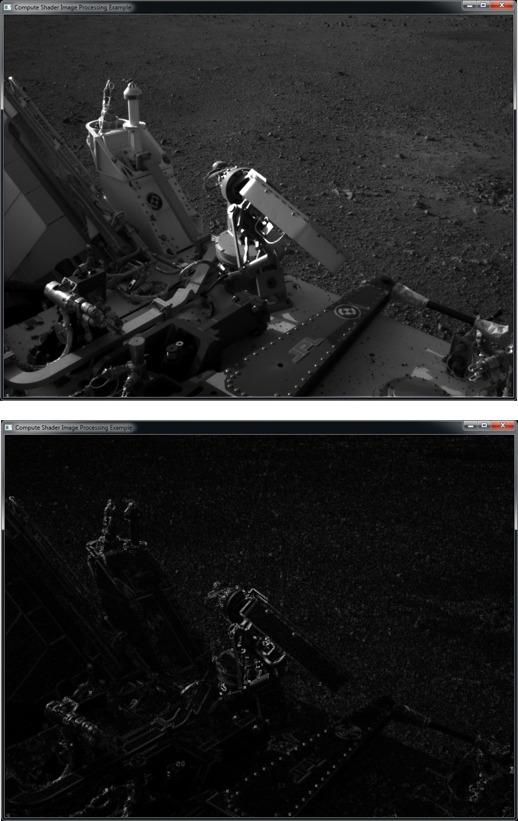
Figure 12.5 Image processing
Input image (top) and resulting output image (bottom), generated by the image-processing compute-shader example.
The image-processing example shader includes a call to barrier after all of the input image data has been read into the shared variable scanline. This ensures that all of the invocations in the local workgroup (including the current invocation’s neighbors) have completed the read from the input image and have written the result into the shared variable. Without the barrier, it is possible to suffer from a race condition where some invocations of the shader will read from the shared variable before the adjacent invocations have completed their writes into it. The result can be sparkling corruption in the output image.
Figure 12.6 shows the result of applying this shader with the call to barrier removed. A horizontal and vertical gridlike pattern of seemingly random pixels is visible. This is due to some invocations of the shader receiving stale or uninitialized data because they move ahead of their neighbors within the local workgroup. The reason that the corruption appears as a gridlike pattern is that the graphics processor used to generate this example processes a number of invocations in lockstep; therefore, those invocations cannot get out of sync. However, the local workgroup is broken up into a number of these subgroups, and they can get ahead of each other. Therefore, we see corrupted pixels produced by the invocations that happen to be executed by the first and last members of the subgroups. If the number of invocations working in lockstep were different, the spacing of the grid pattern would change accordingly.

Figure 12.6 Image processing artifacts
Output of the image processing example, without barriers, showing artifacts.
Chapter Summary
This chapter introduced you to compute shaders. As they are not tied to a specific part of the traditional graphics pipeline and have no fixed intended use, the amount that could be written about compute shaders is enormous. Instead, we covered the basics and provided a couple of examples that should demonstrate how compute shaders may be used to perform the nongraphics parts of your graphics applications.
1. Create a compute shader with glCreateShader() using the type GL_COMPUTE_SHADER.
2. Set the shader source with glShaderSource() and compile it with glCompileShader().
3. Attach it to a program object with glAttachShader() and link it with glLinkProgram().
4. Make the program current with glUseProgram().
5. Launch compute workloads with glDispatchCompute() or glDispatchComputeIndirect().
In your compute shader:
1. Specify the local workgroup size using the local_size_x, local_size_y, and local_size_z input layout qualifiers.
2. Read and write memory by using buffer or image variables or by updating the values of atomic counters.
The special built-in variables available to a compute shader are as follows:
• gl_WorkGroupSize is a constant containing the three-dimensional local size as declared by the input layout qualifiers.
• gl_NumWorkGroups is a copy of the global workgroup count as passed to the glDispatchCompute() or glDispatchCompute() function.
• gl_LocalInvocationID is the coordinate of the current shader invocation within the local workgroup.
• gl_WorkGroupID is the coordinate of the local workgroup within the global workgroup.
• gl_GlobalInvocationID is the coordinate of the current shader invocation within the global workgroup.
• gl_LocalInvocationIndex is a flattened version of gl_LocalInvocationID.
Compute Shader Best Practices
The following are a handful of tips for making effective use of compute shaders. If you follow this advice, your compute shaders are more likely to perform well and work correctly on a wide range of hardware.
Choose the Right Workgroup Size
Choose a local workgroup size that is appropriate for the workload you need to process. Choosing a size that is too large may not allow you to fit everything you need into shared variables. On the other hand, choosing a size that is too small may reduce efficiency, depending on the architecture of the graphics processor.
Use Barriers
Remember to insert control flow and memory barriers before attempting to communicate between compute shader invocations. If you leave out memory barriers, you open your application to the effects of race conditions. It may appear to work on one machine but could produce corrupted data on others.
Utilize Shared Variables
Make effective use of shared variables. Try to structure your workload into blocks—especially if it is memory-intensive and multiple invocations will read the same memory locations. Read blocks of data into shared variables, issue a barrier, and then operate on the data in the shared variable. Write the results back to memory at the end of the shader. Ideally, each memory location accessed by an invocation will be read exactly once and written exactly once.
Do Other Things While Your Compute Shader Runs
If you can, insert graphics work (or even more compute work) between producing data with a compute shader and consuming that data in a graphics shader. Not doing this will force the compute shader to complete execution before the graphics shader can begin execution. By placing unrelated work between the compute shader producer and the graphics shader consumer, that work may be overlapped, improving overall performance.