
Chapter 5. Viewing Transformations, Culling, Clipping, and Feedback
Chapter Objectives
After reading this chapter, you’ll be able to do the following:
• View a three-dimensional geometric model by transforming it to have any size, orientation, and perspective.
• Understand a variety of useful coordinate systems, which ones are required by OpenGL, and how to transform from one to the next.
• Transform surface normals.
• Clip your geometric model against arbitrary planes.
• Capture the geometric result of these transforms before displaying them.
Previous chapters hinted at how to manipulate your geometry to fit into the viewing area on the screen, but we give a complete treatment in this chapter. This includes feedback, the ability to send it back to the application, as well as culling, the removal of objects that can’t be seen, and clipping, the intersection of your geometry with planes either by OpenGL or by you.
Typically, you’ll have many objects with independently specified geometric coordinates. These need to be transformed (moved, scaled, and oriented) into the scene. Then the scene itself needs to be viewed from a particular location, direction, scaling, and orientation.
This chapter contains the following major sections:
• “Viewing” overviews how computer graphics simulates the three-dimensional world on a two-dimensional display.
• “User Transformations” characterizes the various types of transformations that you can employ in shaders to manipulate vertex data.
• “OpenGL Transformations” covers the transformations OpenGL implements.
• “Transform Feedback” describes processing and storing vertex data using vertex-transforming shaders to optimize rendering performance.
Viewing
If we display a typical geometric model’s coordinates directly onto the display device, we probably won’t see much. The range of coordinates in the model (e.g., –100 to +100 meters) will not match the range of coordinates consumed by the display device (e.g., 0 to 1919 pixels), and it is cumbersome to restrict ourselves to coordinates that would match. In addition, we want to view the model from different locations, directions, and perspectives. How do we compensate for this?
Fundamentally, the display is a flat, fixed, two-dimensional rectangle, while our model contains extended three-dimensional geometry. This chapter will show how to project our model’s three-dimensional coordinates onto the fixed two-dimensional screen coordinates.
The key tools for projecting three dimensions down to two are a viewing model, use of homogeneous coordinates, application of linear transformations by matrix multiplication, and a viewport mapping. These tools are discussed in the following sections.
Viewing Model
For the time being, it is important to keep thinking in terms of three-dimensional coordinates while making many of the decisions that determine what is drawn on the screen. It is too early to start thinking about which pixels need to be drawn. Instead, try to visualize three-dimensional space. It is later, after the viewing transformations are completed, after the subjects of this chapter, that pixels will enter the discussion.
Camera Model
The common transformation process for producing the desired view is analogous to taking a photograph with a camera. As shown in Figure 5.1, the steps with a camera (or a computer) might be the following:
1. Move your camera to the location you want to shoot from, and point the camera in the desired direction (viewing transformation).
2. Move the subject to be photographed into the desired location in the scene (modeling transformation).
3. Choose a camera lens or adjust the zoom (projection transformation).
4. Take the picture (apply the transformations).
5. Stretch or shrink the resulting image to the desired picture size (viewport transformation). For 3D graphics, this also includes stretching or shrinking the depth (depth-range scaling). Do not confuse this with Step 3, which selected how much of the scene to capture, not how much to stretch the result.
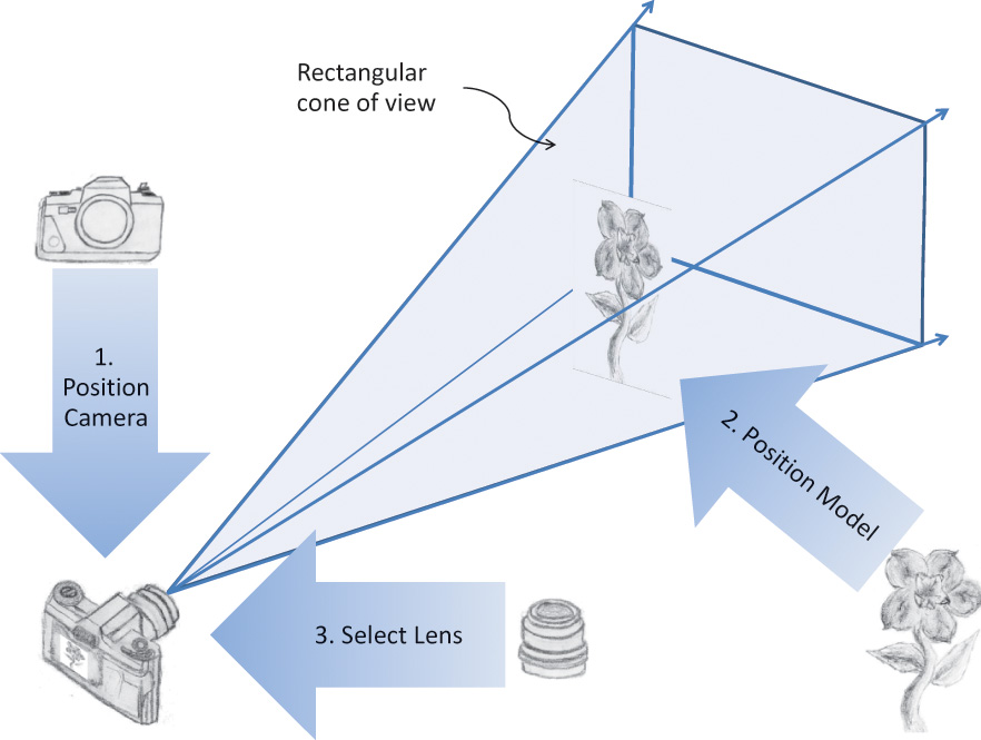
Notice that Steps 1 and 2 can be considered doing the same thing, but in opposite directions. You can leave the camera where you found it and bring the subject in front of it, or leave the subject where it is and move the camera toward the subject. Moving the camera to the left is the same as moving the subject to the right. Twisting the camera clockwise is the same as twisting the subject counterclockwise. It is really up to you which movements you perform as part of Step 1, with the remainder belonging to Step 2. Because of this, these two steps are normally lumped together as the model-view transform. It will, though, always consist of some sequence of movements (translations), rotations, and scalings. The defining characteristic of this combination is in making a single, unified space for all the objects assembled into one scene to view, or eye space.
In OpenGL, you are responsible for doing Steps 1 through 3 in your shaders. That is, you’ll be required to hand OpenGL coordinates with the model-view and projective transformations already done. You are also responsible for telling OpenGL how to do the viewport transformation for Step 5, but the fixed rendering pipeline will do that transformation for you, as described in “OpenGL Transformations” on page 226.
Figure 5.2 summarizes the coordinate systems required by OpenGL for the full process. So far, we have discussed the second box (user transforms) but are showing the rest to set the context for the whole viewing stack, finishing with how you specify your viewport and depth range to OpenGL. The final coordinates handed to OpenGL for culling, clipping, and rasterization are normalized homogeneous coordinates. That is, the coordinates to be drawn will be in the range [–1.0, 1.0] until OpenGL scales them to fit the viewport.
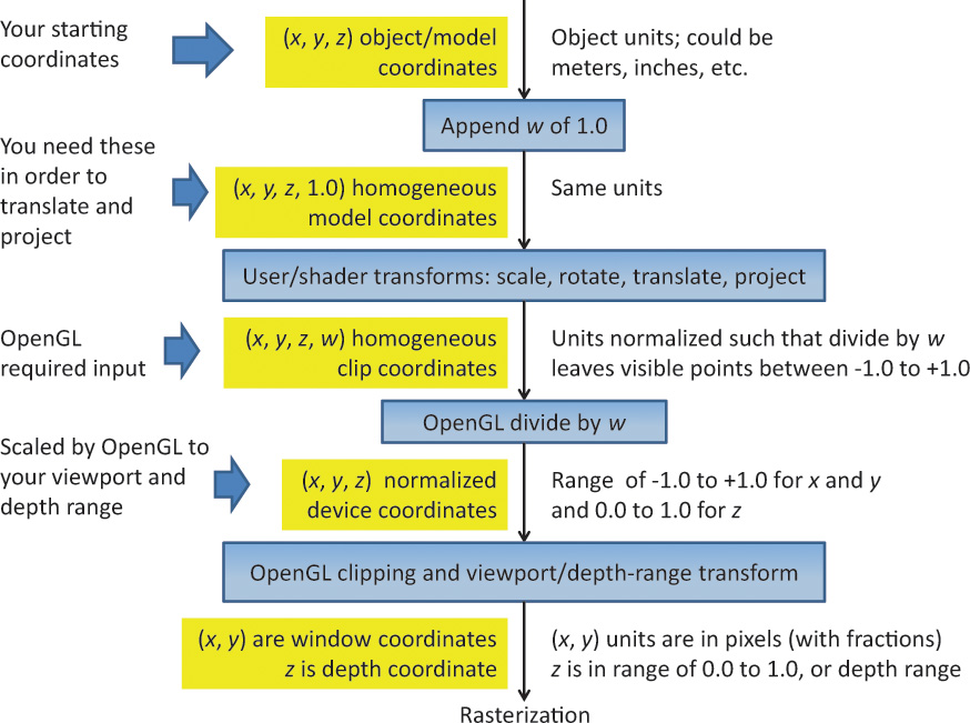
Figure 5.2 Coordinate systems required by OpenGL
The coordinate systems are the boxes on the left. The central boxes transform from one coordinate system to the next. Units are described to the right.
It will be useful to name additional coordinate systems lying within the view, model, and projection transforms. These are no longer part of the OpenGL model, but still highly useful and conventional when using shaders to assemble a scene or calculate lighting. Figure 5.3 shows an expansion of the user transforms box from Figure 5.2. In particular, most lighting calculations done in shaders will be done in eye space. Examples making full use of eye space are provided in Chapter 7, “Light and Shadow.”
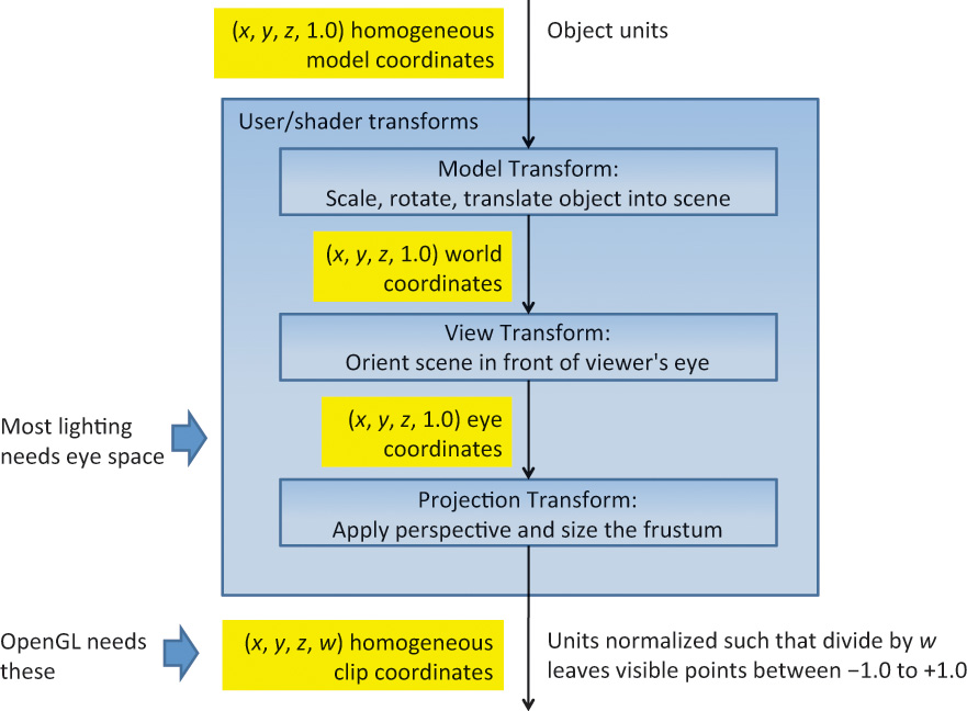
Figure 5.3 User coordinate systems unseen by OpenGL
These coordinate systems, while not used by OpenGL, are still vital for lighting and other shader operations.
Viewing Frustum
Step 3 in our camera analogy is to choose a lens, or zoom amount. This selects how narrow or wide of a rectangular cone through the scene the camera will capture. Only geometry falling within this cone will be in the final picture. At the same time, Step 3 will also produce the information needed (in the homogeneous fourth coordinate, w) to later create the foreshortening effect of perspective.
OpenGL will additionally exclude geometry that is too close or too far away; that is, the geometry in front of a near plane or the geometry behind a far plane. There is no counterpart to this in the camera analogy (other than cleaning foreign objects from inside your lens), but it is helpful in a variety of ways. Most important, objects approaching the cone’s apex appear infinitely large, which causes problems, especially if they should reach the apex. At the other end of this spectrum, objects too far away to be drawn in the scene are best excluded for performance reasons and some depth precision reasons as well, if depth must span too large a distance.
Thus, we have two additional planes intersecting the four planes of the rectangular viewing cone. As shown in Figure 5.4, these six planes define a frustum-shaped viewing volume.
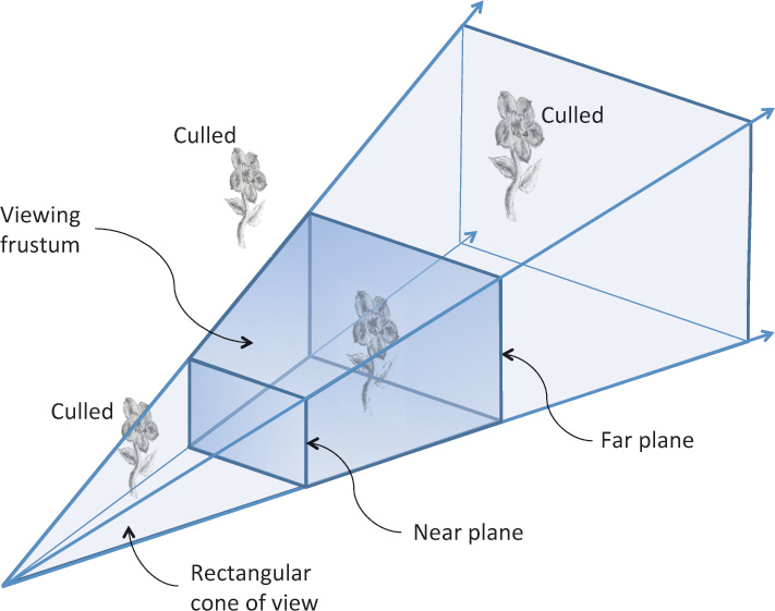
Frustum Clipping
Any primitive falling outside the four planes forming the rectangular viewing cone will not get drawn (culled), as it would fall outside our rectangular display. Further, anything in front of the near plane or behind the far plane will also be culled. What about a primitive that spans both sides of one of these planes? OpenGL will clip such primitives. That is, it will compute the intersection of their geometry with the plane and form new geometry for just the shape that falls within the frustum.
Because OpenGL has to perform this clipping to draw correctly, the application must tell OpenGL where this frustum is. This is part of Step 3 of the camera analogy, where the shader must apply the transformations, but OpenGL must know about it for clipping. There are ways shaders can clip against additional user planes, discussed later, but the six frustum planes are an intrinsic part of OpenGL.
Orthographic Viewing Model
Sometimes, a perspective view is not desired, and an orthographic view is used instead. This type of projection is used by applications for architectural blueprints and computer-aided design, where it’s crucial to maintain the actual sizes of objects and the angles between them as they’re projected. This could be done simply by ignoring one of the x, y, or z coordinates, letting the other two coordinates give two-dimensional locations. You would do that, of course, after orienting the objects and the scene with model-view transformations, as with the camera model. But in the end, you will still need to locate and scale the resulting model for display in normalized device coordinates. The transformation for this is the last one given in the next section.
User Transformations
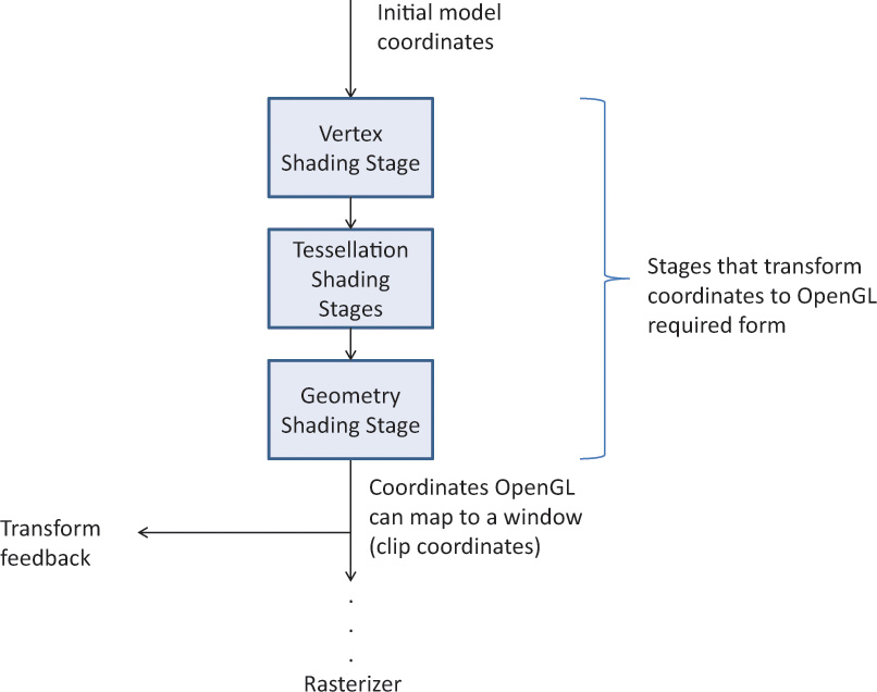
The stages of the rendering pipeline that transform three-dimensional coordinates for OpenGL viewing are shown in Figure 5.5. Essentially, they are the programmable stages appearing before rasterization. Because these stages are programmable, you have a lot of flexibility in the initial form of your coordinates and in how you transform them. However, you are constrained to end with the form the subsequent fixed (nonprogrammable) stages need. That is, we need to make homogeneous coordinates that are ready for perspective division (also referred to as clip coordinates). What that means and how to do it are the subjects of the following sections.
Each of the viewing model steps was called out as a transformation. The steps are all linear transformations that can be accomplished through matrix multiplication on homogeneous coordinates. The upcoming matrix multiplication and homogeneous coordinate sections give refreshers on these topics. Understanding them is the key to truly understanding how OpenGL transformations work.
In a shader, transforming a vertex by a matrix looks like this:
#version 330 core
uniform mat4 Transform; // stays the same for many vertices
// (primitive granularity)
in vec4 Vertex; // per-vertex data sent each time this
// shader is run
void main()
{
gl_Position = Transform * Vertex;
}
Linear transformations can be composed, so just because our camera analogy needed four transformation steps does not mean we have to transform our data four times. Rather, all those transformations can be composed into a single transformation. If we want to transform our model first by transformation matrix A followed by transformation matrix B, we will see we can do so with transformation matrix C, where
C = BA
(Because we are showing examples of matrix multiplication with the vertex on the right and the matrix on the left, composing transforms show up in reverse order: B is applied to the result of applying A to a vertex. The details behind this are explained in the upcoming refresher.)
So the good news is that we can collapse any number of linear transformations into a single matrix multiply, allowing the freedom to think in terms of whatever steps are most convenient.
Matrix Multiply Refresher
For our use, matrices and matrix multiplication are nothing more than a convenient mechanism for expressing linear transformations, which in turn are a useful way to do the coordinate manipulations needed for displaying models. The vital matrix mechanism is explained here, while interesting uses for it will come up in numerous places in subsequent discussions.
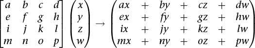
First, a definition. A 4 × 4 matrix takes a 4-component vector to another 4-component vector through multiplication by the following rule:
Now, some observations.
• Each component of the new vector is a linear function of all the components of the old vector—hence the need for 16 values in the matrix.
• The multiply always takes the vector (0, 0, 0, 0) to (0, 0, 0, 0). This is characteristic of linear transformations and shows that if this were a 3 × 3 matrix times a 3-component vector, translation (moving) can’t be done with a matrix multiply. We’ll see how translating a 3-component vector becomes possible with a 4 × 4 matrix and homogeneous coordinates.
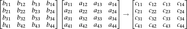
In our viewing models, we will want to take a vector through multiple transformations, here expressed as matrix multiplications by matrices A and then B:
We want to do this efficiently by finding a matrix C such that
v″ = Cv
where
C = BA
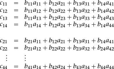
Being able to compose the B transform and the A transform into a single transform C is a benefit we get by sticking to linear transformations. The following definition of matrix multiplication makes all of this work out.
where
cij = bi1a1j + bi2a2j + bi3a3j + bi4a4j
that is
Matrix multiplication is noncommutative: generally speaking, when multiplying matrices and A and B
AB ≠ BA
and, generally, when multiplying matrix A and vector v
Av ≠ vA
so care is needed to multiply in the correct order. Matrix multiplication is, fortunately, associative:
C(BA) = (CB)A = CBA
That’s useful, as accumulated matrix multiplies on a vector can be reassociated.
C(B(Av)) = (CBA)v
This is a key result we will take advantage of to improve performance.
Homogeneous Coordinates
The geometry we want to transform is innately three-dimensional. However, we will gain two key advantages by moving from three-component Cartesian coordinates to four-component homogeneous coordinates. These are 1) the ability to apply perspective and 2) the ability to translate (move) the model using only a linear transform. That is, we will be able to get all the rotations, translations, scaling, and projective transformations we need by doing matrix multiplication if we first move to a 4-coordinate system. More accurately, the projective transformation is a key step in creating perspective, and it is the step we must perform in our shaders. (The final step is performed by the system when it eliminates this new fourth coordinate.)
If you want to understand this and homogeneous coordinates more deeply, read the next section. If you just want to go on some faith and grab 4 × 4 matrices that will get the job done, you can skip to the next section.
Advanced: What Are Homogeneous Coordinates?
Three-dimensional data can be scaled and rotated with linear transformations of three-component vectors by multiplying by 3 × 3 matrices.
Unfortunately, translating (moving/sliding over) three-dimensional Cartesian coordinates cannot be done by multiplying with a 3 × 3 matrix. It requires an extra vector addition to move the point (0, 0, 0) somewhere else. This is a called an affine transformation, which is not a linear transformation. (Recall that any linear transformation maps (0, 0, 0) to (0, 0, 0).) Including that addition means the loss of the benefits of linear transformations, like the ability to compose multiple transformations into a single transformation. So we want to find a way to translate with a linear transformation. Fortunately, by embedding our data in a four-coordinate space, we turn affine transformations back into a simple linear transform (meaning we can move our model laterally using only multiplication by a 4 × 4 matrix).
For example, to move data by 0.3 in the y direction, assuming a fourth vector coordinate of 1.0:
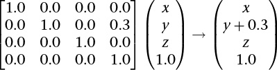
At the same time, we acquire the extra component needed to do perspective.
An homogeneous coordinate has one extra component and does not change the point it represents when all its components are scaled by the same amount.
For example, all these coordinates represent the same point:
(2.0, 3.0, 5.0, 1.0)
(4.0, 6.0, 10.0, 2.0)
(0.2, 0.3, 0.5, 0.1)
In this way, homogeneous coordinates act as directions instead of locations; scaling a direction leaves it pointing in the same direction. This is shown in Figure 5.6. Standing at (0, 0), the homogeneous points (1, 2), (2, 4), and others along that line appear in the same place. When projected onto the 1D space, they all become the point 2.
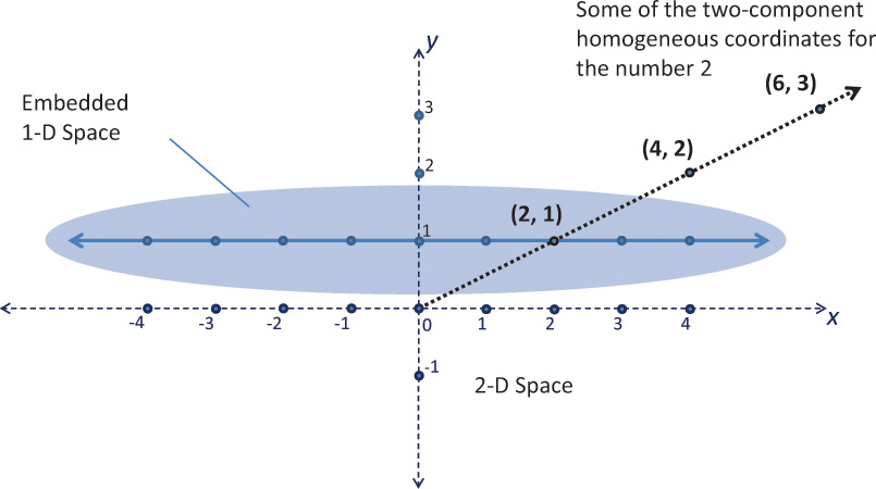
Figure 5.6 One-dimensional homogeneous space
Shows how to embed the 1D space into two dimensions, at the location y = 1, to get homogeneous coordinates.
Skewing is a linear transformation. Skewing Figure 5.6 can translate the embedded 1D space, as shown in Figure 5.7, while preserving the location of (0, 0) in the 2D space. (All linear transforms keep (0, 0) fixed.)

The desire is to translate points in the 1D space with a linear transform. This is impossible within the 1D space, as the point 0 needs to move—something 1D linear transformations cannot do. However, the 2D skewing transformation is linear and accomplishes the goal of translating the 1D space.
If the last component of an homogeneous coordinate is 0, it implies a “point at infinity.” The 1D space has only two such points at infinity: one in the positive direction and one in the negative direction. However, the 3D space, embedded in a 4-coordinate homogeneous space, has a point at infinity for any direction you can point. These points can model the perspective point where two parallel lines (e.g., sides of a building or railroad tracks) would appear to meet. The perspective effects we care about, though, will become visible without our needing to specifically think about this.
We will move to homogeneous coordinates by adding a fourth w component of 1.0,
(2.0, 3.0, 5.0) → (2.0, 3.0, 5.0, 1.0)
and later go back to Cartesian coordinates by dividing all components by the fourth component and dropping the fourth component.
Perspective transforms modify w components to values other than 1.0. Making w larger can make coordinates appear farther away. When it’s time to display geometry, OpenGL will transform homogeneous coordinates back to the three-dimensional Cartesian coordinates by dividing their first three components by the last component. This will make the objects farther away (now having a larger w) have smaller Cartesian coordinates, hence getting drawn on a smaller scale. A w of 0.0 implies (x, y) coordinates at infinity. (The object got so close to the viewpoint that its perspective view got infinitely large.) This can lead to undefined results. There is nothing fundamentally wrong with a negative w; the following coordinates represent the same point.
(2.0, 3.0, 5.0, 1.0)
(–2.0, –3.0, –5.0, –1.0)
But negative w can stir up trouble in some parts of the graphics pipeline, especially if it ever gets interpolated toward a positive w, as that can make it land on or very near 0.0. The simplest way to avoid problems is to keep your w components positive.
Linear Transformations and Matrices
We start our task of mapping into device coordinates by adding a fourth component to our three-dimensional Cartesian coordinates, with a value of 1.0, to make homogeneous coordinates. These coordinates are then ready to be multiplied by one or more 4 × 4 matrices that rotate, scale, translate, and apply perspective. Examples of how to use each of these transforms are given here. The summary is that each of these transformations can be made through multiplication by a 4 × 4 matrix, and a series of such transformations can be composed into a single 4 × 4 matrix, once, that can then be used on multiple vertices.
Translation
Translating an object takes advantage of the fourth component we just added to our model coordinates and of the fourth column of a 4 × 4 transformation matrix. We want a matrix T to multiply all our object’s vertices v by to get translated vertices v′.
v′ = Tv
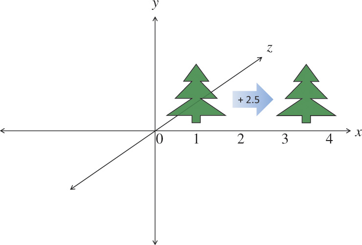
Each component can be translated by a different amount by putting those amounts in the fourth column of T. For example, to translate by 2.5 in the positive x direction, and not at all in the y or z directions:

Then multiplying by a vector v = (x, y, z,1) gives
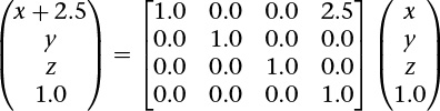
This is demonstrated in Figure 5.8.
Of course, you’ll want such matrix operations encapsulated. There are numerous utilities available for this, and one is included in the accompanying vmath.h. We already used it in Chapter 3, “Drawing with OpenGL.” To create a translation matrix using this utility, call
The following listing shows a use of this.
// Application (C++) code
#include "vmath.h"
.
.
.
// Make a transformation matrix that translates coordinates by (1, 2, 3)
vmath::mat4 translationMatrix = vmath::translate(1.0, 2.0, 3,0);
// Set this matrix into the current program.
glUniformMatrix4fv(matrix_loc, 1, GL_FALSE, translationMatrix);
.
.
.
After going through the next type of transformation, we’ll show a code example for combining transformations with this utility.
Scaling
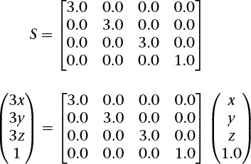
Grow or shrink an object, as in Figure 5.9, by putting the desired scaling factor on the first three diagonal components of the matrix. Making a scaling matrix S, which applied to all vertices v in an object, would change its size.
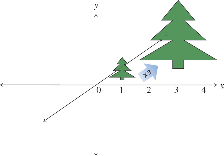
Figure 5.9 Scaling an object to three times its size
Note that if the object is off center, this also moves its center three times further from (0, 0, 0).
The following example makes geometry 3 times larger.
Note that nonisomorphic scaling is easily done, as the scaling is per component, but it would be rare to do so when setting up your view and model transforms. (If you want to stretch results vertically or horizontally, do that at the end with the viewport transformation. Doing it too early would make shapes change when they rotate.) Note that when scaling, we didn’t scale the w component, as that would result in no net change to the point represented by the homogeneous coordinate (since in the end, all components are divided by w).
If the object being scaled is not centered at (0, 0, 0), the simple matrix above will also move it farther from or closer to (0, 0, 0) by the scaling amount. Usually, it is easier to understand what happens when scaling if you first center the object on (0, 0, 0). Then scaling leaves it in the same place while changing its size. If you want to change the size of an off-center object without moving it, first translate its center to (0, 0, 0), then scale it, and finally translate it back. This is shown in Figure 5.10.

Figure 5.10 Scaling an object in place
Scale in place by moving to (0, 0, 0), scaling, and then moving it back.
This would use three matrices: T, S, and T–1, for translate to (0, 0, 0), scale, and translate back, respectively. When each vertex v of the object is multiplied by each of these matrices in turn, the final effect is that the object would change size in place, yielding a new set of vertices v′:
v′ = T–1(S(Tv))
or
v′ = (T–1ST)v
which allows for premultiplication of the three matrices into a single matrix.
M = T–1ST
v′ = Mv
M now does the complete job of scaling an off-center object.
To create a scaling transformation with the included utility, you can use
The resulting matrix can be directly multiplied by another such transformation matrix to compose them into a single matrix that performs both transformations.
// Application (C++) code
#include "vmath.h"
.
.
.
// Compose translation and scaling transforms
vmath::mat4 translateMatrix = vmath::translate(1.0, 2.0, 3,0);
vmath::mat4 scaleMatrix = vmath::scale(5.0);
vmath::mat4 scaleTranslateMatrix = scaleMatrix * translateMatrix;
.
.
.
Any sequence of transformations can be combined into a single matrix this way.
Rotation
Rotating an object follows a similar scheme. We want a matrix R that when applied to all vertices v in an object will rotate it. The following example, shown in Figure 5.11, rotates 50 degrees counterclockwise around the z axis. Figure 5.12 shows how to rotate an object without moving its center instead of also revolving it around the z axis.
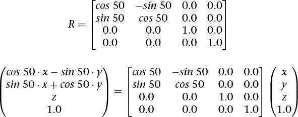
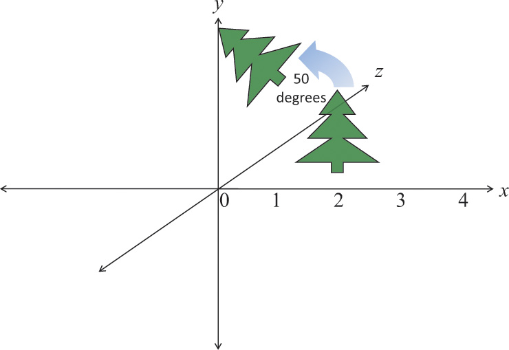
Figure 5.11 Rotation
Rotating an object 50 degrees in the xy plane, around the z axis. Note that if the object is off center, it also revolves the object around the point (0, 0, 0).
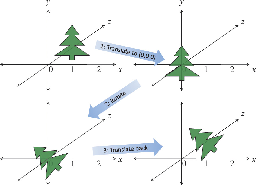
Figure 5.12 Rotating in place
Rotating an object in place by moving it to (0, 0, 0), rotating, and then moving it back.
When rotating around the z axis, the vertices in the object keep their z values the same, rotating in the xy plane. To rotate instead around the x axis by an amount θ:
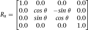
To rotate around the y axis:

In all cases, the rotation is in the direction of the first axis toward the second axis—that is, from the row with the cos –sin pattern to the row with the sin cos pattern, for the positive axes corresponding to these rows.
If the object being rotated is not centered at (0, 0, 0), the matrices will also rotate the whole object around (0, 0, 0), changing its location. Again, as with scaling, it’ll be easier to first center the object on (0, 0, 0). So again, translate it to (0, 0, 0), transform it, and then translate it back. This could use three matrices, T, R, and T–1, to translate to (0, 0, 0), rotate, and translate back.
v′ = T–1(R(Tv))
or
v′ = (T–1RT)v
which again allows for the premultiplication into a single matrix.
To create a rotation transformation with the included utility, you can use
Perspective Projection
This one is a bit tougher. We now assume viewing and modeling transformations are completed, with larger z values meaning objects are farther away.
We will consider the following two cases:
1. Symmetric, centered frustum, where the z-axis is centered in the cone.
2. Asymmetric frustum, like seeing what’s through a window when you look near it but not toward its middle.
For all, the viewpoint is now at (0, 0, 0), looking generally toward the positive z direction.
First, however, let’s consider an oversimplified (hypothetical) perspective projection.

Note the last matrix row replaces the w (fourth) coordinate with the z coordinate. This will make objects with a larger z (farther away) appear smaller when the division by w occurs, creating a perspective effect. However, this particular method has some shortcomings. For one, all z values will end up at 1.0, losing information about depth. We also didn’t have much control over the cone we are projecting and the rectangle we are projecting onto. Finally, we didn’t scale the result to the [–1.0, 1.0] range expected by the viewport transform. The remaining examples take all this into account.
So we consider now a fuller example for OpenGL, using a symmetric centered frustum. We refer to our view frustum, shown again with the size of the near plane labeled in Figure 5.13.
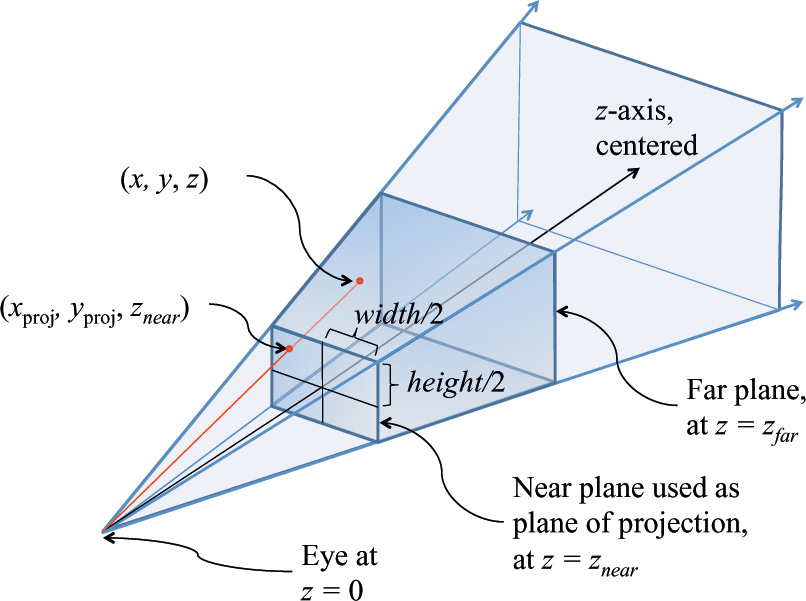
We want to project points in the frustum onto the near plane, directed along straight lines going toward (0, 0, 0). Any straight line emanating from (0, 0, 0) keeps the ratio if z to x the same for all its points, and similarly for the ratio of z to y. Thus, the (xproj, yproj) value of the projection on the near plane will keep the ratios of ![]() and
and ![]() . We know there is an upcoming division by depth to eliminate homogeneous coordinates, so solving for xproj while still in the homogeneous space simply gives xproj = x · znear. Similarly, yproj = y · znear. If we then include a divide by the size of the near plane to scale the near plane to the range of [–1.0, 1.0], we end up with the requisite first two diagonal elements shown in the projection transformation matrix.
. We know there is an upcoming division by depth to eliminate homogeneous coordinates, so solving for xproj while still in the homogeneous space simply gives xproj = x · znear. Similarly, yproj = y · znear. If we then include a divide by the size of the near plane to scale the near plane to the range of [–1.0, 1.0], we end up with the requisite first two diagonal elements shown in the projection transformation matrix.
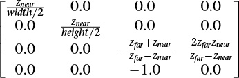
(This could also be computed from the angle of the viewing cone, if so desired.)
Finally, we consider the second perspective projection case: the asymmetric frustum. This is the fully general frustum, when the near plane might not be centered on the z axis. The z axis could even be completely outside it, as mentioned earlier when looking at an interior wall next to a window. Your direction of view is the positive z axis, which is not going through the window. You see the window off to the side, with an asymmetric perspective view of what’s outside the window. In this case, points on the near plane are already in the correct location, but those farther away need to be adjusted for the fact that the projection in the near plane is off center. You can see this adjustment in the third column of the matrix, which moves the points an amount based on how off-center the near-plane projection is, scaled by how far away the points are (because this column multiplies by z).

All these steps—rotate, scale, translate, project, and possibly others—will make matrices that can be multiplied together into a single matrix. Now with one multiplication by this new matrix, we can simultaneously scale, translate, rotate, and apply the perspective projection.
To create a perspective projection transformation with the included utility, there are a couple of choices. You can have full control using a frustum call, or you can more casually and intuitively create one with the lookat call.
The resulting vectors, still having four coordinates, are the homogeneous coordinates expected by the OpenGL pipeline.
The final step in projecting the perspective view onto the screen is to divide the (x, y, z) coordinates in v′ by the w coordinate in v′, for every vertex. However, this is done internally by OpenGL; it is not something you do in your shaders.
Orthographic Projection
With an orthographic projection, the viewing volume is a rectangular parallelpiped, or, more informally, a box (see Figure 5.14). Unlike in perspective projection, the size of the viewing volume doesn’t change from one end to the other, so distance from the camera doesn’t affect how large an object appears.

Figure 5.14 Orthographic projection
Starts with straightforward projection of the parallelpiped onto the front plane. x, y, and z will need to be scaled to fit into [–1, 1], [–1, 1], and [0, 1], respectively. This will be done by dividing by the sizes of the width, height, and depth in the model.
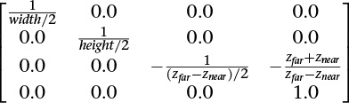
This is done after all the translation, scaling, and rotation is done to look in the positive z direction to see the model to view. With no perspective, we will keep the w as it is (1.0), accomplished by making the bottom row of the transformation matrix (0, 0, 0, 1). We will still scale z to lie within [0, 1] so z-buffering can hide obscured objects, but neither z nor w will have any effect on the screen location. That leaves scaling x from the width of the model to [–1, 1] and similarly for y. For a symmetric volume (positive z going down the middle of the parallelpiped), this can be done with the following matrix:
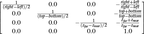
For the case of the positive z not going down the middle of the view (but still looking parallel to the z axis to see the model), the matrix is just slightly more complex. We use the diagonal to scale and the fourth column to center.
To create an orthographic projection transformation with the included utility, you can use
Transforming Normals
In addition to transforming vertices, we need to transform surface normals—that is, vectors that point in the direction perpendicular to a surface at some point. In perhaps one of the most confusing twists of terminology, normals are often required to be normalized—that is, of length 1.0. However, the “normal” meaning perpendicular and the “normal” in normalize are completely unrelated, and we will come upon needs for normalized normals when computing lighting.
Typically, when computing lighting, a vertex will have a normal associated with it, so the lighting calculation knows what direction the surface reflects light. Shaders doing these calculations appear in Chapter 7, “Light and Shadow.” Here, though, we will discuss the fundamentals of transforming them by taking them through rotations, scaling, and so on along with the vertices in a model.
Normal vectors are typically only 3-component vectors; not using homogeneous coordinates. For one thing, translating a surface does not change its normal, so normals don’t care about translation, removing one of the reasons we used homogeneous coordinates. Because normals are mostly used for lighting, which we complete in a pre-perspective space, we remove the other reason we use homogeneous coordinates (projection).
Perhaps counterintuitively, normal vectors aren’t transformed in the same way that vertices or position vectors are. Imagine a surface at an angle that gets stretched by a transformation. Stretching makes the angle of the surface shallower, which changes the perpendicular direction in the opposite way from applying the same stretching to the normal. This would happen, for example, if you stretch a sphere to make an ellipse. We need to come up with a different transformation matrix to transform normals than the one we used for vertices.
So how do we transform normals? To start, let M be the 3 × 3 matrix that has all the rotations and scaling needed to transform your object from model coordinates to eye coordinates before transforming for perspective. This would be the upper 3 × 3 block in your 4 × 4 transformation matrix before compounding translation or projection transformations into it. Then, to transform normals, use the following equation:
n′ = M–1Tn
That is, take the transpose of the inverse of M and use that to transform your normals. If all you did was rotation and isometric (non-shape-changing) scaling, you could transform directions with just M.
They’d be scaled by a different amount, but no doubt a normalize call in their future will even that out.
OpenGL Matrices
While shaders know how to multiply matrices, the API in the OpenGL core profile does not manipulate matrices beyond setting them, possibly transposed, into uniform and per-vertex data to be used by your shaders. It is up to you to build up the matrices you want to use in your shader, which you can do with the included helper routines as described in the previous section.
You will want to be multiplying matrices in your application before sending them to your shaders, for a performance benefit. Suppose that you need matrices to do the following transformations:
1. Move the camera to the right view: translate and rotate.
2. Move the model into view: translate, rotate, and scale.
3. Apply perspective projection.
That’s a total of six matrices. You can use a vertex shader to do this math, as shown in Example 5.1.
Example 5.1 Multiplying Multiple Matrices in a Vertex Shader
#version 330 core
uniform mat4 ViewT, ViewR, ModelT, ModelR, ModelS, Project;
in vec4 Vertex;
void main()
{
gl_Position = Project
* ModelS * ModelR * ModelT
* ViewR * ViewT
* Vertex;
}
However, that’s a lot of arithmetic to do for each vertex. Fortunately, the intermediate results for many vertices will be the same each time. To the extent that consecutive transforms (matrices) are staying the same for a large number of vertices, you’ll want to instead precompute their composition (product) in your application and send the single resulting matrix to your shader.
// Application (C++) code
#include "vmath.h"
.
.
.
vmath::mat4 ViewT = vmath::rotate(...)
vmath::mat4 ViewR = vmath::translate(...);
vmath::mat4 View = ViewR * ViewT;
vmath::mat4 ModelS = vmath::scale(...);
vmath::mat4 ModelR = vmath::rotate(...);
vmath::mat4 ModelT = vmath::translate(...);
vmath::mat4 Model = ModelS * ModelR * ModelT;
vmath::mat4 Project = vmath::frustum(...);
vmath::mat4 ModelViewProject = Project * Model * View;
An intermediate situation might be to have a single-view transformation and a single-perspective projection, but multiple-model transformations. You might do this if you reuse the same model to make many instances of an object in the same view.
#version 330 core
uniform mat4 View, Model, Project;
in vec4 Vertex;
void main()
{
gl_Position = View * Model * Project * Vertex;
}
In this situation, the application would change the model matrix more frequently than the others. This will be economical if enough vertices are drawn per change of the matrix Model. If only a few vertices are drawn per instance, it will be faster to send the model matrix as a vertex attribute.
#version 330 core
uniform mat4 View, Project;
in vec4 Vertex;
in mat4 Model; // a transform sent per vertex
void main()
{
gl_Position = View * Model * Project * Vertex;
}
(Another alternative for creating multiple instances is to construct the model transformation within the vertex shader based on the built-in variable gl_InstanceID. This was described in detail in Chapter 3, “Drawing with OpenGL.”)
Of course, when you can draw a large number of vertices all with the same cumulative transformation, you’ll want to do only one multiply in the shader.
#version 330 core
uniform mat4 ModelViewProject;
in vec4 Vertex;
void main()
{
gl_Position = ModelViewProject * Vertex;
}
Matrix Rows and Columns in OpenGL
The notation used in this book corresponds to the broadly used traditional matrix notation. We stay true to this notation, regardless of how data is set into a matrix. A column will always mean a vertical slice of a matrix when written in this traditional notation.
Beyond notation, matrices have semantics for setting and accessing parts of a matrix, and these semantics are always column-oriented. In a shader, using array syntax on a matrix yields a vector with values coming from a column of the matrix
mat3x4 m; // 3 columns, 4 rows
vec4 v = m[1]; // v is initialized to the second column of m
Note
Neither the notation we use nor these column-oriented semantics is to be confused with column-major order and row-major order, which refer strictly to memory layout of the data behind a matrix. The memory layout has nothing to do with our notation in this book and nothing to do with the language semantics of GLSL: You will probably not know whether, internally, a matrix is stored in column-major or row-major order.
Caring about column-major or row-major memory order will come up only when you are in fact laying out the memory backing a GLSL matrix yourself. This is done when setting matrices in a uniform block. As was shown in Chapter 2, “Shader Fundamentals,” when discussing uniform blocks, you use layout qualifiers row_major and column_major to control how GLSL will load the matrix from this memory.
Because OpenGL is not creating or interpreting your matrices, you can treat them as you wish. If you want to transform a vertex by matrix multiplication with the matrix on the right,
#version 330 core
uniform mat4 M;
in vec4 Vertex;
void main()
{
gl_Position = Vertex * M; // nontraditional order of multiplication
}
then, as expected, gl_Position.x will be formed by the dot product of Vertex and the first column of matrix M, and so on for gl_Position y, z, and w components transformed by the second, third, and fourth columns. However, we stick to the tradition of keeping the matrix on the left and the vertices on the right.
Note
GLSL vectors automatically adapt to being either row vectors or column vectors, depending on whether they are on the left side or right side of a matrix multiply, respectively. In this way, they are different from a one-column or one-row matrix.
OpenGL Transformations
To tell OpenGL where you want the near and far planes, use the glDepthRange() commands.
The underlying windowing system of your platform, not OpenGL, is responsible for opening a window on the screen. However, by default, the viewport is set to the entire pixel rectangle of the window that’s opened. You use glViewport() to choose a smaller drawing region; for example, you can subdivide the window to create a split-screen effect for multiple views in the same window.
Multiple Viewports
You will sometimes want to render a scene through multiple viewports. OpenGL has commands to support doing this, and the geometry shading stage can select which viewport subsequent rendering will target. More details and an example are given in “Multiple Viewports and Layered Rendering” on page 562.
Advanced: z Precision
One bizarre effect of these transformations is z fighting. The hardware’s floating-point numbers used to do the computation have limited precision. Hence, depth coordinates that are mathematically distinct end up having the same (or even reversed) actual floating-point z values. This in turn causes incorrectly hidden objects in the depth buffer. The effect varies per pixel and can cause disturbing flickering intersections of nearby objects. Precision of z is made even worse with perspective division, which is applied to the depth coordinate along with all the other coordinates: As the transformed depth coordinate moves farther away from the near clipping plane, its location becomes increasingly less precise, as shown in Figure 5.15.
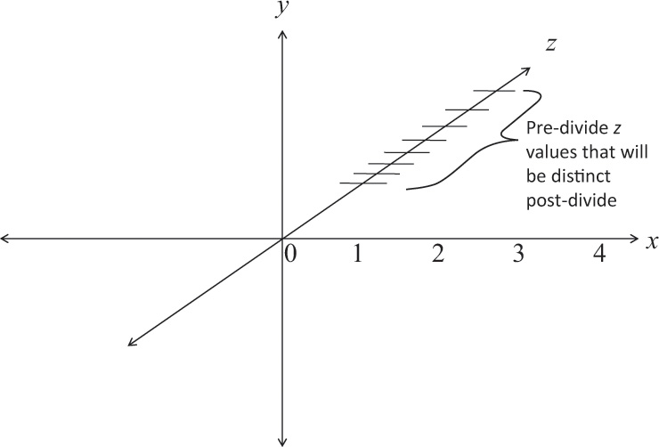
Figure 5.15 z precision
An exaggerated showing of adjacent, distinctly representable depths, assuming an upcoming perspective division.
Even without perspective division, there is a finite granularity to floating-point numbers, but the divide makes it worse and nonlinear, resulting in more severe problems at greater depths. The bottom line is that it is possible to ask for too much or too small a range of z values. To avoid this, take care to keep the far plane as close to the near plane as possible, and don’t compress the z values into a narrower range than necessary.
Advanced: User Culling and Clipping
OpenGL automatically culls and clips geometry against the near and far planes as well as the viewport. User culling and user clipping refer to adding additional planes at arbitrary orientations, intersecting your geometry, such that the display sees the geometry on one side of the plane but not on the other side. You would use a culling plane to remove primitives that fall on one side of it, and you might use a clipping plane, for example, to show a cutaway of a complex object.
OpenGL user culling and clipping are a joint effort between OpenGL and special built-in shader arrays, gl_CullDistance[] and gl_ClipDistance[], which you are responsible for writing to. These variables let you control where vertices are in relation to a plane. Normal interpolation then assigns distances to the fragments between the vertices. Example 5.2 shows a straightforward use of gl_ClipDistance[].
Example 5.2 Simple Use of gl_ClipDistance
#version 450 core
uniform vec4 Plane; // A, B, C, and D for Ax + By + Cz + D = 0
in vec4 Vertex; // w == 1.0
float gl_ClipDistance[1]; // declare use of 1 clip plane.
void main()
{
// evaluate plane equation
gl_ClipDistance[0] = dot(Vertex, Plane);
// or use gl_CullDistance[0] for culling
}
The convention is that a distance of 0 means the vertex is on the plane, a positive distance means the vertex is inside (the keep it side) of the clip or cull plane, and a negative distance means the point is outside (the cull-it side) of the clip or cull plane. The distances will be linearly interpolated across the primitive. OpenGL will cull entire primitives lying entirely on the outside of any one of the cull planes. (The space for keeping primitives is the intersection of the inside of all the cull planes.) Further, OpenGL will cull all fragments whose interpolated clip distance is less than 0.
Each array element of the gl_ClipDistance array, and each element of the gl_CullDistance array, represents one plane. There are a limited number of planes, likely around eight or more, that typically must be shared between gl_ClipDistance elements and gl_CullDistance elements. That is, you might have eight clip distances available, or eight cull distances available, or four of each, or two of one and six of the other, but never more than a total of eight between the two arrays. In general, the total number allowed is given by gl_MaxCombinedClipAndCullDistances, while the number allowed for culling is gl_MaxCullDistances, and the number allowed for clipping is gl_MaxClipDistances.
Note that these built-in variables are declared with no size, yet the number of used planes (array elements) comes from the shader. This means you must either redeclare these arrays with a specific size or access them only with compile-time constant indexes. This size established how many planes are in play.
All shaders in all stages that declare or use gl_ClipDistance[] should make the array the same size, and similarly for gl_CullDistances[]. This size needs to include all the clip planes that are enabled via the OpenGL API; if the size does not include all enabled planes, results are undefined. To enable OpenGL clipping of the clip plane written to in Example 5.2, enable the following enumerant in your application:
glEnable(GL_CLIP_PLANE0);
There are also other enumerates, like GL_CLIP_PLANE1, GL_CLIP_PLANE2. These enumerants are organized sequentially, so that GL_CLIP_PLANEi is equal to GL_CLIP_PLANE0 + i. This allows programmatic selection of which and how many user clip or cull planes to use. Your shaders should write to all the enabled planes, or you’ll end up with odd implementation behavior.
The built-in variables gl_CullDistance and gl_ClipDistance are also available in a fragment shader, allowing fragments to read their interpolated distances from each plane.
Controlling OpenGL Transformations
Many of OpenGL’s fixed-function operations take place in clip space, which is the space in which your vertex shader (or tessellation or geometry shaders, if enabled) produce coordinates. By default, OpenGL maps the clip-space coordinate (0, 0) to the center of window space, with positive x coordinates pointing right and positive y coordinates pointing up. This places the (–1, –1) coordinate at the bottom left of the window and (1, 1) at the top right. Think of this as a piece of graph paper: The positive y direction in mathematics, architecture and other engineering fields is up. However, many graphical systems treat positive y as pointing downward as an artifact of how early cathode ray tubes scanned the electron beam across the screen. The layout of data in video memory meant that it was convenient to make y point down.
Further, for consistency and orthogonality, just as the range –1.0 to 1.0 maps to the visible x and y ranges, so –1.0 to 1.0 maps to the visible depth range, with –1.0 being the near plane and 1.0 being the far plane. Unfortunately, because of the way that floating-point numbers work, most precision is offered near 0.0, which is somewhere far from the viewer, although we’d really like to have most of our depth precision close to the viewer—at the near plane. Again, some other graphics systems use this alternative mapping where negative z coordinates in clip space are behind the viewer and the visible depth range maps to 0.0 to 1.0 in clip space.
OpenGL allows you to reconfigure either or both of these mappings using a single call to glClipControl(), the prototype of which is
Transform Feedback
Transform feedback can be considered a stage of the OpenGL pipeline that sits after all of the vertex-processing stages and directly before primitive assembly and rasterization.1 Transform feedback captures vertices as they are assembled into primitives (points, lines, or triangles) and allows some or all of their attributes to be recorded into buffer objects. In fact, the minimal OpenGL pipeline that produces useful work is a vertex shader with transform feedback enabled; no fragment shader is necessary. Each time a vertex passes through primitive assembly, those attributes that have been marked for capture are recorded into one or more buffer objects. Those buffer objects can then be read back by the application or their contents used in subsequent rendering passes by OpenGL.
1. To be more exact, transform feedback is tightly integrated into the primitive assembly process as whole primitives are captured into buffer objects. This is seen as buffers run out of space and partial primitives are discarded. For this to occur, some knowledge of the current primitive type is required in the transform feedback stage.
Transform Feedback Objects
The state required to represent transform feedback is encapsulated into a transform feedback object. This state includes the buffer objects that will be used for recording the captured vertex data, counters indicating how full each buffer object is, and state indicating whether transform feedback is currently active. A transform feedback object is created by reserving a transform feedback object name and then binding it to the transform feedback object binding point on the current context. To reserve transform feedback object names, call
The parameter n specifies how many transform feedback object names are to be created, and ids specifies the address of an array where the reserved names will be placed. If you want only one name, you can set n to one and pass the address of a GLuint variable in ids. Once you have created a transform feedback object, it contains the default transform feedback state and can be bound, at which point it is ready for use. To bind a transform feedback object to the context, call
This binds the transform feedback object named id to the binding on the context indicated by target, which in this case must be GL_TRANSFORM_FEEDBACK. To determine whether a particular value is the name of a transform feedback object, you can call glIsTransformFeedback(), whose prototype is as follows:
Once a transform feedback object is bound, all commands affecting transform feedback state affect that transform feedback object. It’s not necessary to have a transform feedback object bound in order to use transform feedback functionality, as there is a default transform feedback object. The default transform feedback object assumes the id zero, so passing zero as the id parameter to glBindTransformFeedback() returns the context to use the default transform feedback object (unbinding any previously bound transform feedback object in the process). However, as more complex uses of transform feedback are introduced, it becomes convenient to encapsulate the state of transform feedback into transform feedback objects. Therefore, it’s good practice to create and bind a transform feedback object even if you intend to use only one.
Once a transform feedback object is no longer needed, it should be deleted by calling
This function deletes the n transform feedback objects whose names are stored in the array whose address is passed in ids. Deletion of the object is deferred until it is no longer in use. That is, if the transform feedback object is active when glDeleteTransformFeedbacks() is called, it is not deleted until transform feedback is ended.
Transform Feedback Buffers
Transform feedback objects are primarily responsible for managing the state representing capture of vertices into buffer objects. This state includes which buffers are bound to the transform feedback buffer binding points. Multiple buffers can be bound simultaneously for transform feedback, and subsections of buffer objects can also be bound. It is even possible to bind different subsections of the same buffer object to different transform feedback buffer binding points simultaneously. To bind an entire buffer object to one of the transform feedback buffer binding points, call
The index parameter should be set to the index of the transform feedback buffer binding point to which to bind the transform feedback object. The name of the buffer to bind is passed in buffer. The total number of binding points is an implementation-dependent constant that can be discovered by querying the value of GL_MAX_TRANSFORM_FEEDBACK_BUFFERS, and index must be less than this value. All OpenGL implementations must support at least 64 transform feedback buffer binding points. It’s also possible to bind a range of a buffer object to one of the transform feedback buffer binding points by calling
Again, index should be between zero and one less than the value of GL_MAX_TRANSFORM_FEEDBACK_BUFFERS, and buffer contains the name of the buffer object to bind. The offset and size parameters define which section of the buffer object to bind. This functionality can be used to bind different ranges of the same buffer object to different transform feedback buffer binding points. Care should be taken that the ranges do not overlap. Attempting to perform transform feedback into multiple, overlapping sections of the same buffer object will result in undefined behavior, possibly including data corruption or worse.
In order to allocate a transform feedback buffer, use code that is similar to what’s shown in Example 5.3.
Example 5.3 Example Initialization of a Transform Feedback Buffer
// Create a new buffer object
GLuint buffer;
glCreateBuffers(1, &buffer);
// Call glNamedBufferStorage to allocate 1MB of space
glNamedBufferStorage(buffer, // buffer
1024 * 1024, // 1 MB
NULL, // no initial data
0); // flags
// Now we can bind it to indexed buffer binding points.
glTransformFeedbackBufferRange(xfb, // object
0, // index 0
buffer, // buffer name
0, // start of range
512 * 1024); // first half of buffer
glTransformFeedbackBufferRange(xfb, // object
1, // index 1
buffer, // same buffer
512 * 1024, // start half way
512 * 1024); // second half
Notice how in Example 5.3, the newly created buffer object name is first used with a call to glNamedBufferStorage() to allocate space. The data parameter to glNamedBufferStorage() is set to NULL to indicate that we wish to simply allocate space but do not wish to provide initial data for the buffer. In this case, the buffer’s contents will initially be undefined. Also, we set the flags parameter of glNamedBufferStorage() to zero. This tells the OpenGL implementation about the intended use for the buffer object: We’re not going to map this buffer object or change its content from the CPU, and we want the OpenGL driver to optimize its allocation for that scenario. This should give the implementation enough information to intelligently allocate memory for the buffer object in an optimal manner for it to be used for transform feedback.
Once the buffer has been created and space has been allocated for it, sections of it are bound to the indexed transform feedback buffer binding points by calling glTransformFeedbackBufferRange() twice: once to bind the first half of the buffer to the first binding point and again to bind the second half of the buffer to the second binding point. This demonstrates why the buffer needs to be created and allocated before using it with glTransformFeedbackBufferRange(). glTransformFeedbackBufferRange() takes an offset, size parameters describing a range of the buffer object that must lie within the buffer object. This cannot be determined if the object does not yet exist.
In Example 5.3, we call glBindBufferRange() twice in a row. In this simple example, this might not be a concern, but OpenGL does provide a shortcut for the times when you want to bind a lot of ranges or a lot of buffers. The glBindBuffersRange() function can be used to bind a sequence of ranges of the same or different buffers to different indexed binding points on a single target. Its prototype is
Configuring Transform Feedback Varyings
While the buffer bindings used for transform feedback are associated with a transform feedback object, the configuration of which outputs of the vertex (or geometry) shader are to be recorded into those buffers is stored in the active program object.
There are two methods of specifying which varyings will be recorded during transform feedback:
• Through the OpenGL API, using glTransformFeedbackVaryings()
• Through the shader, using xfb_buffer, xfb_offset, and xfb_stride
For writing new code, you might find the declarative style in the shader to be more straightforward. However, you can pick which method you like best; just use only one method at a time. The methods are discussed next.
Configuring Transform Feedback Varyings Through the OpenGL API
To specify through the OpenGL API which varyings will be recorded during transform feedback, call
In this function, program specifies the program object that will be used for transform feedback. varyings contains an array of strings that represent the names of varying variables that are outputs of the shader that are to be captured by transform feedback. count is the number of strings in varyings. bufferMode is a token indicating how the captured varyings should be allocated to transform feedback buffers. If bufferMode is set to GL_INTERLEAVED_ATTRIBS, all of the varyings will be recorded one after another into the buffer object bound to the first transform feedback buffer binding point on the current transform feedback object. If bufferMode is GL_SEPARATE_ATTRIBS, each varying will be captured into its own buffer object.
An example of the use of glTransformFeedbackVaryings() is shown in Example 5.4.
Example 5.4 Application Specification of Transform Feedback Varyings
// Create an array containing the names of varyings to record
static const char * const vars[] =
{
"foo", "bar", "baz"
};
// Call glTransformFeedbackVaryings
glTransformFeedbackVaryings(prog,
sizeof(vars) / sizeof(vars[0]),
varyings,
GL_INTERLEAVED_ATTRIBS);
// Now the program object is set up to record varyings squashed
// together in the same buffer object. Alternatively, we could call...
glTransformFeedbackVaryings(prog,
sizeof(vars) / sizeof(vars[0]),
varyings,
GL_SEPARATE_ATTRIBS);
// This sets up the varyings to be recorded into separate buffers.
// Now (this is important), link the program object...
// ... even if it's already been linked before.
glLinkProgram(prog);
InExample 5.4, there is a call to glLinkProgram() directly after the call to glTransformFeedbackVaryings(). This is because the selection of varyings specified in the call to glTransformFeedbackVaryings() does not take effect until the next time the program object is linked. If the program has previously been linked and is then used without being relinked, no errors will occur, but nothing will be captured during transform feedback.2
2. Calling glTransformFeedbackVaryings() after a program object has already been linked and then not linking it again is a common error made even by experienced OpenGL programmers.
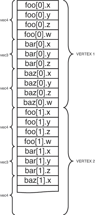
After the code in Example 5.4 has been executed, whenever prog is in use while transform feedback is active, the values written to foo, bar, and baz will be recorded into the transform feedback buffers bound to the current transform feedback object. In the case where the bufferMode parameter is set to GL_INTERLEAVED_ATTRIBS, the values of foo, bar, and baz will be tightly packed into the buffer bound to the first transform feedback buffer binding point, as shown in Figure 5.16.
However, if bufferMode is GL_SEPARATE_ATTRIBS, each of foo, bar, and baz will be packed tightly into its own buffer object, as shown in Figure 5.17.

In both cases, the attributes will be tightly packed together. The amount of space in the buffer object that each varying consumes is determined by its type in the vertex shader. That is, if foo is declared as a vec3 in the vertex shader, it will consume exactly three floats in the buffer object. In the case where bufferMode is GL_INTERLEAVED_ATTRIBS, the value of bar will be written immediately after the value of foo. In the case where bufferMode is GL_SEPARATE_ATTRIBS, the values of foo will be tightly packed into one buffer with no gaps between them (as will the values of bar and baz).
This seems rather rigid. There are cases where you may wish to align the data written into the transform feedback buffer differently from default (leaving unwritten gaps in the buffer). There may also be cases where you would want to record more than one variable into one buffer but record other variables into another. For example, you may wish to record foo and bar into one buffer while recording baz into another. In order to increase the flexibility of transform feedback varying setup and allow this kind of usage, some special variable names reserved by OpenGL signal to the transform feedback subsystem that you wish to leave gaps in the output buffer or to move between buffers. These are gl_SkipComponents1, gl_SkipComponents2, gl_SkipComponents3, gl_SkipComponents4, and gl_NextBuffer. When any of the gl_SkipComponents variants is encountered, OpenGL will leave a gap for the number of components specified (1, 2, 3, or 4) in the transform feedback buffer. These variable names can be used when bufferMode is GL_INTERLEAVED_ATTRIBS. Example 5.5 shows an example of using this.
Example 5.5 Leaving Gaps in a Transform Feedback Buffer
// Declare the transform feedback varying names
static const char * const vars[] =
{
"foo",
"gl_SkipComponents2",
"bar",
"gl_SkipComponents3",
"baz"
};
// Set the varyings
glTransformFeedbackVaryings(prog,
sizeof(vars) / sizeof(vars[0]),
varyings,
GL_INTERLEAVED_ATTRIBS);
// Remember to link the program object
glLinkProgram(prog);
When the other special variable name, gl_NextBuffer, is encountered, OpenGL will start allocating varyings into the buffer bound to the next transform feedback buffer. This allows multiple varyings to be recorded into a single buffer object. Additionally, if gl_NextBuffer is encountered when bufferMode is GL_SEPARATE_ATTRIBS, or if two or more instances of gl_NextBuffer are encountered in a row in GL_INTERLEAVED_ATTRIBS, OpenGL allows a whole binding point to be skipped and nothing recorded into the buffer bound there. An example of gl_NextBuffer is shown in Example 5.6.
Example 5.6 Assigning Transform Feedback Outputs to Different Buffers
// Declare the transform feedback varying names
static const char * const vars[] =
{
"foo", "bar" // Variables to record into buffer 0
"gl_NextBuffer", // Move to binding point 1
"baz" // Variable to record into buffer 1
};
// Set the varyings
glTransformFeedbackVaryings(prog,
sizeof(vars) / sizeof(vars[0]),
varyings,
GL_INTERLEAVED_ATTRIBS);
// Remember to link the program object
glLinkProgram(prog);
The special variables names gl_SkipComponentsN and gl_NextBuffer can be combined to allow very flexible vertex layouts to be created. If it is necessary to skip over more than four components, multiple instances of gl_SkipComponents may be used back to back. Care should be taken with aggressive use of gl_SkipComponents, though, because skipped components still contribute toward the count of the count of the number of components captured during transform feedback, even though no data is actually written. This may cause a reduction in performance or even a failure to link a program. If there is a lot of unchanged, static data in a buffer, it may be preferable to separate the data into static and dynamic parts and leave the static data in its own buffer object(s), allowing the dynamic data to be more tightly packed.
Finally, Example 5.7 shows an (albeit rather contrived) example of the combined use of gl_SkipComponents and gl_NextBuffer, and Figure 5.18 shows how the data ends up laid out in the transform feedback buffers.
Example 5.7 Assigning Transform Feedback Outputs to Different Buffers
// Declare the transform feedback varying names
static const char * const vars[] =
{
// Record foo, a gap of 1 float, bar, and then two floats
"foo", "gl_SkipComponents1, "bar", "gl_SkipComponents2"
// Move to binding point 1
"gl_NextBuffer",
// Leave a gap of 4 floats, then record baz, then leave
// another gap of 2 floats
"gl_SkipComponents4" "baz", "gl_SkipComponents2"
// Move to binding point 2
"gl_NextBuffer",
// Move directly to binding point 3 without directing anything
// to binding point 2
"gl_NextBuffer",
// Record iron and copper with a 3 component gap between them
"iron", "gl_SkipComponents3", "copper"
};
// Set the varyings
glTransformFeedbackVaryings(prog,
sizeof(vars) / sizeof(vars[0]),
varyings,
GL_INTERLEAVED_ATTRIBS);
// Remember to link the program object
glLinkProgram(prog);

As you can see in Example 5.7, gl_SkipComponents can come between varyings or at the start or end of the list of varyings to record into a single buffer. Putting a gl_SkipComponents variant-first in the list of varyings to capture will result in OpenGL leaving a gap at the front of the buffer before it records data (and then a gap between each sequence of varyings). Also, multiple gl_NextBuffer variables can come back to back, causing a buffer binding point to be passed over and nothing recorded into that buffer. The resulting output layout is shown in Figure 5.18.
Configuring Transform Feedback Varyings Through the Shader
It can be more natural and more expressive to explicitly declare the transform feedback buffer(s) in your shader code than to use the API function glTransformFeedbackVaryings(). To configure transform feedback varyings in a shader, don’t use the entry point glTransformFeedbackVaryings() at all. Instead, use the following shader layout qualifiers:
• xfb_buffer to say which buffer varyings will go to
• xfb_offset to say where in a buffer a varying goes to
• xfb_stride to say how the data is spaced from one vertex to the next
These can be used as in the following examples. Example 5.8 uses a single buffer, corresponding to Figure 5.16, while Example 5.9 uses separate buffers, corresponding to Figure 5.17.
Example 5.8 Shader Declaration of Transform Feedback in a Single Buffer
// layout in a single buffer with individual variables
layout(xfb_offset=0) out vec4 foo; // default xfb_buffer is 0
layout(xfb_offset=16) out vec3 bar;
layout(xfb_offset=28) out vec4 barz;
// or do the same using a block
layout(xfb_offset=0) out { // means all members get an offset
vec4 foo;
vec3 bar; // goes to the next available offset
vec4 barz;
} captured;
Example 5.9 Shader Declaration of Transform Feedback in Multiple Buffers
// layout in a multiple buffers
layout(xfb_buffer=0, xfb_offset=0) out vec4 foo; // must say xfb_offset
layout(xfb_buffer=1, xfb_offset=0) out vec3 bar;
layout(xfb_buffer=2, xfb_offset=0) out vec4 barz;
To capture an output, you must use xfb_offset either directly on the output variable or block member, or on the block declaration to capture all members of the block. That is, the indication of what to capture and what to not capture is given by whether or not it has or inherited an xfb_offset.
Declaring “holes” or padding in the buffer, is quite straightforward. Padding between vertices is established simply by declaring the stride you want for vertices in the buffer, using xfb_stride. Within a block of vertex data, create holes (or skipped data) simply by assigning the exact offset where you want each capturing varying to be stored. Example 5.10 corresponds to Figure 5.18.
Example 5.10 Shader Declaration of Transform Feedback Varyings in Multiple Buffers
// layout in a multiple buffers with holes
layout(xfb_buffer=0, xfb_stride=40, xfb_offset=0) out vec4 foo;
layout(xfb_buffer=0, xfb_stride=40, xfb_offset=20) out vec3 bar;
layout(xfb_buffer=1, xfb_stride=40, xfb_offset=16) out vec4 barz;
layout(xfb_buffer=2, xfb_stride=44) out {
layout(xfb_offset=0) vec4 iron;
layout(xfb_offset=28) vec4 copper;
vec4 zinc; // not captured, not xfb_offset
};
Strides and offsets have to be multiples of 4 unless any double-precision (double) types are involved, in which case they must all be multiples of 8. A single buffer can, of course, have only one stride, so all xfb_stride for a buffer must match. When working with one buffer at a time, you can specify default buffers and strides, for example, by declaring without a variable:
layout(xfb_buffer=1, xfb_stride=40) out;
Subsequent use of xfb_offset will pick up these defaults for the buffer and stride.
Starting and Stopping Transform Feedback
Transform feedback can be started and stopped, and even paused. As might be expected, starting transform feedback when it is not paused causes it to start recording into the bound transform feedback buffers from the beginning. However, starting transform feedback when it is already paused causes it to continue recording from wherever it left off. This is useful to allow multiple components of a scene to be recorded into transform feedback buffers with other components that are not to be recorded rendered in between.
To start transform feedback, call glBeginTransformFeedback().
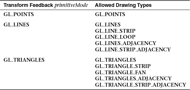
The glBeginTransformFeedback() function starts transform feedback on the currently bound transform feedback object. The primitiveMode parameter must be GL_POINTS, GL_LINES, or GL_TRIANGLES and must match the primitive type expected to arrive at primitive assembly. Note that it does not need to match the primitive mode used in subsequent draw commands if tessellation or a geometry shader is active because those stages might change the primitive type mid-pipeline. That will be covered in Chapters 9 and 10. For the moment, just set the primitiveMode to match the primitive type you plan to draw with. Table 5.1 shows the allowed combinations of primitiveMode and draw command modes.
Once transform feedback is started, it is considered to be active. It may be paused by calling glPauseTransformFeedback(). When transform feedback is paused, it is still considered active but will not record any data into the transform feedback buffers. There are also several restrictions about changing state related to transform feedback while transform feedback is active but paused:
• The currently bound transform feedback object may not be changed.
• It is not possible to bind different buffers to the GL_TRANSFORM_FEEDBACK_BUFFER binding points.
• The current program object cannot be changed.3
3. Actually, it is possible to change the current program object, but an error will be generated by glResumeTransformFeedback() if the program object that was current when glBeginTransformFeedback() was called is no longer current. So be sure to put the original program object back before calling glResumeTransformFeedback().
glPauseTransformFeedback() will generate an error if transform feedback is not active or if it is already paused. To restart transform feedback while it is paused, glResumeTransformFeedback() must be used (not glBeginTransformFeedback()). Likewise, glResumeTransformFeedback() will generate an error if it is called when transform feedback is not active or if it is active but not paused.
When you’ve completed rendering all of the primitives for transform feedback, you change back to normal rendering mode by calling glEndTransformFeedback().
Transform Feedback Example—Particle System
This section contains the description of a moderately complex use of transform feedback. The application uses transform feedback in two ways to implement a particle system. On a first pass, transform feedback is used to capture geometry as it passes through the OpenGL pipeline. The captured geometry is then used in a second pass along with another instance of transform feedback in order to implement a particle system that uses the vertex shader to perform collision detection between particles and the rendered geometry. A schematic of the system is shown in Figure 5.19.
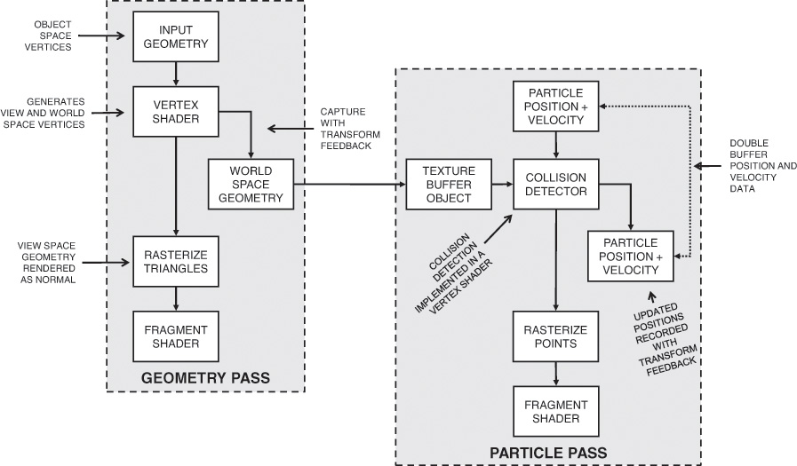
In this application, the particle system is simulated in world space. In a first pass, a vertex shader is used to transform object space geometry into both world space (for later use in the particle system simulation) and into eye space for rendering. The world space results are captured into a buffer using transform feedback, while the eye space geometry is passed through to the rasterizer. The buffer containing the captured world space geometry is attached to a texture buffer object (TBO) so that it can be randomly accessed in the vertex shader that is used to implement collision detection in the second, simulation pass. Using this mechanism, any object that would normally be rendered can be captured so long as the vertex (or geometry) shader produces world space vertices in addition to eye space vertices. This allows the particle system to interact with multiple objects, potentially with each rendered using a different set of shaders—perhaps even with tessellation enabled or other procedurally generated geometry.4
4. Be careful: Tessellation can generate a very large amount of geometry, all of which the simulated particles must be tested against, which could severely affect performance and increase storage requirements for the intermediate geometry.
The second pass is where the particle system simulation occurs. Particle position and velocity vectors are stored in a pair of buffers. Two buffers are used so that data can be double-buffered, as it’s not possible to update vertex data in place. Each vertex in the buffer represents a single particle in the system. Each instance of the vertex shader performs collision detection between the particle (using its velocity to compute where it will move to during the time-step) and all of the geometry captured during the first pass. It calculates new position and velocity vectors, which are captured using transform feedback and written into a buffer object ready for the next step in the simulation.
Example 5.11 contains the source of the vertex shader used to transform the incoming geometry into both world and eye space, and Example 5.12 shows how transform feedback is configured to capture the resulting world space geometry.
Example 5.11 Vertex Shader Used in Geometry Pass of Particle System Simulator
#version 420 core
uniform mat4 model_matrix;
uniform mat4 projection_matrix;
layout (location = 0) in vec4 position;
layout (location = 1) in vec3 normal;
out vec4 world_space_position;
out vec3 vs_fs_normal;
void main(void)
{
vec4 pos = (model_matrix * (position * vec4(1.0, 1.0, 1.0, 1.0)));
world_space_position = pos;
vs_fs_normal = normalize((model_matrix * vec4(normal, 0.0)).xyz);
gl_Position = projection_matrix * pos;
};
Example 5.12 Configuring the Geometry Pass of the Particle System Simulator
static const char * varyings2[] =
{
"world_space_position"
};
glTransformFeedbackVaryings(render_prog, 1, varyings2,
GL_INTERLEAVED_ATTRIBS);
glLinkProgram(render_prog);
During the first geometry pass, the code in Examples 5.11 and 5.12 will cause the world space geometry to be captured into a buffer object. Each triangle in the buffer is represented by three vertices5 that are read (three at a time) during the second pass into the vertex shader and used to perform line segment against triangle intersection test. A TBO is used to access the data in the intermediate buffer so that the three vertices can be read in a simple for loop. The line segment is formed by taking the particle’s current position and using its velocity to calculate where it will be at the end of the time step. This is performed for every captured triangle. If a collision is found, the point’s new position is reflected about the plane of the triangle to make it “bounce” off the geometry.
5. Only triangles are used here. It’s not possible to perform a meaningful physical collision detection between a line segment and another line segment or a point. Also, individual triangles are required for this to work. If strips or fans are present in the input geometry, it may be necessary to include a geometry shader in order to convert the connected triangles into independent triangles.
Example 5.13 contains the code of the vertex shader used to perform collision detection in the simulation pass.
Example 5.13 Vertex Shader Used in Simulation Pass of Particle System Simulator
#version 420 core
uniform mat4 model_matrix;
uniform mat4 projection_matrix;
uniform int triangle_count;
layout (location = 0) in vec4 position;
layout (location = 1) in vec3 velocity;
out vec4 position_out;
out vec3 velocity_out;
uniform samplerBuffer geometry_tbo;
uniform float time_step = 0.02;
bool intersect(vec3 origin, vec3 direction, vec3 v0, vec3 v1, vec3 v2,
out vec3 point)
{
vec3 u, v, n;
vec3 w0, w;
float r, a, b;
u = (v1 - v0);
v = (v2 - v0);
n = cross(u, v);
w0 = origin - v0;
a = -dot(n, w0);
b = dot(n, direction);
r = a / b;
if (r < 0.0 || r > 1.0)
return false;
point = origin + r * direction;
float uu, uv, vv, wu, wv, D;
uu = dot(u, u);
uv = dot(u, v);
vv = dot(v, v);
w = point - v0;
wu = dot(w, u);
wv = dot(w, v);
D = uv * uv - uu * vv;
float s, t;
s = (uv * wv - vv * wu) / D;
if (s < 0.0 || s > 1.0)
return false;
t = (uv * wu - uu * wv) / D;
if (t < 0.0 || (s + t) > 1.0)
return false;
return true;
}
vec3 reflect_vector(vec3 v, vec3 n)
{
return v - 2.0 * dot(v, n) * n;
}
void main(void)
{
vec3 acceleration = vec3(0.0, -0.3, 0.0);
vec3 new_velocity = velocity + acceleration * time_step;
vec4 new_position = position + vec4(new_velocity * time_step, 0.0);
vec3 v0, v1, v2;
vec3 point;
int i;
for (i = 0; i < triangle_count; i++)
{
v0 = texelFetch(geometry_tbo, i * 3).xyz;
v1 = texelFetch(geometry_tbo, i * 3 + 1).xyz;
v2 = texelFetch(geometry_tbo, i * 3 + 2).xyz;
if (intersect(position.xyz, position.xyz - new_position.xyz,
v0, v1, v2, point))
{
vec3 n = normalize(cross(v1 - v0, v2 - v0));
new_position = vec4(point
+ reflect_vector(new_position.xyz -
point, n), 1.0);
new_velocity = 0.8 * reflect_vector(new_velocity, n);
}
}
if (new_position.y < -40.0)
{
new_position = vec4(-new_position.x * 0.3, position.y + 80.0,
0.0, 1.0);
new_velocity *= vec3(0.2, 0.1, -0.3);
}
velocity_out = new_velocity * 0.9999;
position_out = new_position;
gl_Position = projection_matrix * (model_matrix * position);
};
The code to set up transform feedback to capture the updated particle position and velocity vectors is shown in Example 5.14.
Example 5.14 Configuring the Simulation Pass of the Particle System Simulator
static const char * varyings[] =
{
"position_out", "velocity_out"
};
glTransformFeedbackVaryings(update_prog, 2, varyings,
GL_INTERLEAVED_ATTRIBS);
glLinkProgram(update_prog);
The inner rendering loop of the application is quite simple. First, the program object used for rendering the geometry is bound, as is a transform feedback object representing the state required to capture the world space geometry. Then all of the solid objects in the scene are rendered, causing the intermediate buffer to be filled with world space geometry. Next, the program object used for updating particle positions is made current, as is the transform feedback object used for capturing position and velocity data for the particle system. Finally, the particles are rendered. Example 5.15 shows the code for this inner loop.
Example 5.15 Main Rendering Loop of the Particle System Simulator
glUseProgram(render_prog);
glUniformMatrix4fv(render_model_matrix_loc, 1, GL_FALSE, model_matrix);
glUniformMatrix4fv(render_projection_matrix_loc, 1, GL_FALSE,
projection_matrix);
glBindVertexArray(render_vao);
glBindBufferBase(GL_TRANSFORM_FEEDBACK_BUFFER, 0, geometry_vbo);
glBeginTransformFeedback(GL_TRIANGLES);
object.Render();
glEndTransformFeedback();
glUseProgram(update_prog);
glUniformMatrix4fv(model_matrix_loc, 1, GL_FALSE, model_matrix);
glUniformMatrix4fv(projection_matrix_loc, 1, GL_FALSE,
projection_matrix);
glUniform1i(triangle_count_loc, object.GetVertexCount() / 3);
if ((frame_count & 1) != 0)
{
glBindVertexArray(vao[1]);
glBindBufferBase(GL_TRANSFORM_FEEDBACK_BUFFER, 0, vbo[0]);
}
else
{
glBindVertexArray(vao[0]);
glBindBufferBase(GL_TRANSFORM_FEEDBACK_BUFFER, 0, vbo[1]);
}
glBeginTransformFeedback(GL_POINTS);
glDrawArrays(GL_POINTS, 0, min(point_count, (frame_count >> 3)));
glEndTransformFeedback();
glBindVertexArray(0);
frame_count++;
The result of the program is shown in Figure 5.20.
