
Chapter 7. Light and Shadow
Chapter Objectives
After reading this chapter, you’ll be able to do the following:
• Code a spectrum of fragment shaders to light surfaces with ambient, diffuse, and specular lighting from multiple light sources.
• Migrate lighting code between fragment and vertex shaders, based on quality and performance trade-offs.
• Use a single shader to apply a collection of lights to a variety of materials.
• Select among a variety of alternative lighting models.
• Have the objects in your scene cast shadows onto other objects.
In the real world, we see things because they reflect light from a light source or because they are light sources themselves. In computer graphics, just as in real life, we won’t be able to see an object unless it is illuminated by or emits light. We will explore how the OpenGL Shading Language can help us implement such models so that they can execute at interactive rates on programmable graphics hardware.
This chapter contains the following major sections:
• “Lighting Introduction” historically frames the lighting discussions.
• “Classic Lighting Model” shows lighting fundamentals, first based on doing light computations in a fragment shader and then in both the vertex and fragment shaders. This section also shows how to handle multiple lights and materials in a single shader.
• “Advanced Lighting Models” introduces a sampling of advanced methods for lighting a scene including hemisphere lighting, image-based lighting, and spherical harmonics. These can be layered on top of the classic lighting model to create hybrid models.
• “Shadow Mapping” shows a key technique for adding shadows to a scene.
Lighting Introduction
The programmability of OpenGL shaders allows virtually limitless possibilities for lighting a scene. Old-school fixed-functionality lighting models were comparatively constraining, lacking in some realism and in performance-quality trade-offs. Programmable shaders can provide far superior results, especially in the area of realism. Nevertheless, it is still important to start with an understanding of the classic lighting model that was embodied by old fixed functionality, though we will be more flexible on which shader stages do which part. This lighting model still provides the fundamentals on which most rasterization lighting techniques are based and is a springboard for grasping the more advanced techniques.
In that light, we will first show a number of simple shaders that each perform some aspect of the classic lighting model, with the goal being that you may pick and choose the techniques you want in your scene, combine them, and incorporate them into your shaders. Viewing transformations and other aspects of rendering are absent from these shaders so that we may focus just on lighting.
In the later examples of this chapter, we explore a variety of more complex shaders that provide more flexible results. But even with these more flexible shaders, we are limited only by our imaginations. Keep exploring new lighting methods on your own.
Classic Lighting Model
The classic lighting model adds up a set of independently computed lighting components to get a total lighting effect for a particular spot on a material surface. These components are ambient, diffuse, and specular. Each is described in this section, and Figure 7.1 shows them visually.

Figure 7.1 Elements of the classic lighting model
Ambient (top left) plus diffuse (top right) plus specular (bottom) light adding to an overall realistic effect.
Ambient light is light that does not come from any specific direction. The classic lighting model considers it a constant throughout the scene, forming a decent first approximation to the scattered light present in a scene. Computing it does not involve any analysis of the direction of light sources or the direction of the eye observing the scene. It could either be accumulated as a base contribution per light source or be precomputed as a single global effect.
Diffuse light is light scattered by the surface equally in all directions for a particular light source. Diffuse light is responsible for being able to see a surface lit by a light even if the surface is not oriented to reflect the light source directly toward your eye. It doesn’t matter which direction the eye is, but it does matter which direction the light is. It is brighter when the surface is more directly facing the light source, simply because that orientation collects more light than an oblique orientation. Diffuse light computation depends on the direction of the surface normal and the direction of the light source, but not the direction of the eye. It also depends on the color of the surface.
Specular highlighting is light reflected directly by the surface. This highlighting refers to how much the surface material acts like a mirror. A highly polished metal ball reflects a very sharp bright specular highlight, while a duller polish reflects a larger, dimmer specular highlight, and a cloth ball would reflect virtually none at all. The strength of this angle-specific effect is referred to as shininess. Computing specular highlights requires knowing how close the surface’s orientation is to the needed direct reflection between the light source and the eye; hence, it requires knowing the surface normal, the direction of the light source, and the direction of the eye. Specular highlights might or might not incorporate the color of the surface. As a first approximation, it is more realistic to not involve any surface color, making it purely reflective. The underlying color will be present anyway from the diffuse term, giving it the proper tinge.
Fragment Shaders for Different Light Styles
We’ll next discuss how fragment shaders compute the ambient, diffuse, and speculative amounts for several types of light, including directional lighting, point lighting, and spotlight lighting. These will be complete with a vertex and fragment shader pair built up as we go from simplest to more complex. The later shaders may seem long, but if you start with the simplest and follow the incremental additions, it will be easy to understand.
Note: The comments in each example highlight the change or difference from the previous step, making it easy to look and identify the new concepts.
No Lighting
We start with the simplest lighting—no lighting! By this, we don’t mean everything will be black, but that we just draw objects with color unmodulated by any lighting effects. This is inexpensive, occasionally useful, and the base we’ll build on. Unless your object is a perfect mirror, you’ll need this color as the basis for upcoming lighting calculations; all lighting calculations will somehow modulate this base color. It is a simple matter to set a per-vertex color in the vertex shader that will be interpolated and displayed by the fragment shader, as shown in Example 7.1.
Example 7.1 Setting Final Color Values with No Lighting
--------------------------- Vertex Shader -----------------------------
// Vertex shader with no lighting
#version 330 core
uniform mat4 MVPMatrix; // model-view-projection transform
in vec4 VertexColor; // sent from the application, includes alpha
in vec4 VertexPosition; // pretransformed position
out vec4 Color; // sent to the rasterizer for interpolation
void main()
{
Color = VertexColor;
gl_Position = MVPMatrix * VertexPosition;
}
-------------------------- Fragment Shader ----------------------------
// Fragment shader with no lighting
#version 330 core
in vec4 Color; // interpolated between vertices
out vec4 FragColor; // color result for this fragment
void main()
{
FragColor = Color;
}
In the cases of texture mapping or procedural texturing, the base color will come from sending texture coordinates instead of a color, using those coordinates to manifest the color in the fragment shader. Or, if you set up material properties, the color will come from an indexed material lookup. Either way, we start with an unlit base color.
Ambient Light
The ambient light doesn’t change across primitives, so we will pass it in from the application as a uniform variable.
It’s a good time to mention that light itself has color, not just intensity. The color of the light interacts with the color of the surface being lit. This interaction of the surface color by the light color is modeled well by multiplication. Using 0.0 to represent black and 1.0 to represent full intensity enables multiplication to model expected interaction. This is demonstrated for ambient light in Example 7.2.
It is okay for light colors to go above 1.0, especially as we start adding up multiple sources of light. We will start now using the min() function to saturate the light at white. This is important if the output color is the final value for display in a framebuffer. However, if it is an intermediate result, skip the saturation step now, and save it for application to a final color when that time comes.
--------------------------- Vertex Shader -----------------------------
// Vertex shader for ambient light
#version 330 core
uniform mat4 MVPMatrix;
in vec4 VertexColor;
in vec4 VertexPosition;
out vec4 Color;
void main()
{
Color = VertexColor;
gl_Position = MVPMatrix * VertexPosition;
}
-------------------------- Fragment Shader ----------------------------
// Fragment shader for global ambient lighting
#version 330 core
uniform vec4 Ambient; // sets lighting level, same across many vertices
in vec4 Color;
out vec4 FragColor;
void main()
{
vec4 scatteredLight = Ambient; // this is the only light
// modulate surface color with light, but saturate at white
FragColor = min(Color * scatteredLight, vec4(1.0));
}
You probably have an alpha (fourth component) value in your color that you care about, and don’t want it modified by lighting. So unless you’re after specific transparency effects, make sure your ambient color has as an alpha of 1.0, or just include only the r, g, and b components in the computation. For example, the two lines of code in the fragment shader could read
vec3 scatteredLight = vec3(Ambient); // this is the only light
vec3 rgb = min(Color.rgb * scatteredLight, vec3(1.0));
FragColor = vec4(rgb, Color.a);
which passes the Color alpha component straight through to the output FragColor alpha component, modifying only the r, g, and b components. We will generally do this in the subsequent examples.
A keen observer might notice that scatteredLight could have been multiplied by Color in the vertex shader instead of the fragment shader. For this case, the interpolated result would be the same. Because the vertex shader usually processes fewer vertices than the number of fragments processed by the fragment shader, it would probably run faster too. However, for many lighting techniques, the interpolated results will not be the same. Higher quality will be obtained by computing per fragment rather than per vertex. It is up to you to make this performance vs. quality trade-off, probably by experimenting with what is best for a particular situation. We will first show the computation in the fragment shader and then discuss optimizations (approximations) that involve moving computations up into the vertex shader or even to the application. Feel free to put them whereever is best for your situation.
Directional Light
If a light is far, far away, it can be approximated as having the same direction from every point on our surface. We refer to such a light as directional. Similarly, if a viewer is far, far away, the viewer (eye) can also be approximated as having the same direction from every point on our surface. These assumptions simplify the math, so the code to implement a directional light is simple and runs faster than the code for other types of lights. This type of light source is useful for mimicking the effects of a light source like the sun.
We start with the ambient light computation from the previous example and add on the effects for diffuse scattering and specular highlighting. We compute these effects for each fragment of the surface we are lighting. Again, just like with ambient light, the directional light will have its own color, and we will modulate the surface color with this light color for the diffuse scattering. The specular contribution will be computed separately to allow the specular highlights to be the color of the light source, not modulated by the color of the surface.
The scattered and reflected amounts we need to compute vary with the cosine of the angles involved. Two vectors in the same direction form an angle of 0° with a cosine of 1.0. This indicates a completely direct reflection. As the angle widens, the cosine moves toward 0.0, indicating less reflected light. Fortunately, if our vectors are normalized (having a length of 1.0), these cosines are computed with a simple dot product, as shown in Example 7.3. The surface normal will be interpolated between vertices, though it could also come from a texture map or an analytic computation. The far away light-source assumption lets us pass in the light direction as the uniform variable LightDirection. For a far-away light and eye, the specular highlights all peak for the same surface-normal direction. We compute this direction once in the application and pass it in through the uniform variable HalfVector. Then cosines of this direction with the actual surface normal are used to start specular highlighting.
Shininess for specular highlighting is measured with an exponent used to sharpen the angular fall-off from a direct reflection. Squaring a number less than 1.0 but near to 1.0 makes it closer to 0.0. Higher exponents sharpen the effect even more—that is, leaving only angles near 0°, whose cosine is near 1.0, with a final specular value near 1.0. The other angles decay quickly to a specular value of 0.0. Hence, we see the desired effect of a shiny spot on the surface. Overall, higher exponents dim the amount of computed reflection, so in practice, you’ll probably want to use either a brighter light color or an extra multiplication factor to compensate. We pass such defining specular values as uniform variables because they are surface properties that are constant across the surface.
The only way either a diffuse reflection component or a specular reflection component can be present is if the angle between the light-source direction and the surface normal is in the range [–90.0°,90.0°]: a normal at 90° means the surface itself is edge-on to the light. Tip it a bit further, and no light will hit it. As soon as the angle grows beyond 90°, the cosine goes below 0. We determine the angle by examining the variable diffuse. This is set to the greater of 0.0 and the cosine of the angle between the light-source direction and the surface normal. If this value ends up being 0.0, the value that determines the amount of specular reflection is set to 0.0 as well. Recall we assume that the direction vectors and surface normal vector are normalized, so the dot product between them yields the cosine of the angle between them.
Example 7.3 Directional Light Source Lighting
--------------------------- Vertex Shader -----------------------------
// Vertex shader for a directional light computed in the fragment shader
#version 330 core
uniform mat4 MVPMatrix;
uniform mat3 NormalMatrix; // to transform normals, pre-perspective
in vec4 VertexColor;
in vec3 VertexNormal; // we now need a surface normal
in vec4 VertexPosition;
out vec4 Color;
out vec3 Normal; // interpolate the normalized surface normal
void main()
{
Color = VertexColor;
// transform the normal, without perspective, and normalize it
Normal = normalize(NormalMatrix * VertexNormal);
gl_Position = MVPMatrix * VertexPosition;
}
-------------------------- Fragment Shader ----------------------------
// Fragment shader computing lighting for a directional light
#version 330 core
uniform vec3 Ambient;
uniform vec3 LightColor;
uniform vec3 LightDirection; // direction toward the light
uniform vec3 HalfVector; // surface orientation for shiniest spots
uniform float Shininess; // exponent for sharping highlights
uniform float Strength; // extra factor to adjust shininess
in vec4 Color;
in vec3 Normal; // surface normal, interpolated between vertices
out vec4 FragColor;
void main()
{
// compute cosine of the directions, using dot products,
// to see how much light would be reflected
float diffuse = max(0.0, dot(Normal, LightDirection));
float specular = max(0.0, dot(Normal, HalfVector));
// surfaces facing away from the light (negative dot products)
// won't be lit by the directional light
if (diffuse == 0.0)
specular = 0.0;
else
specular = pow(specular, Shininess); // sharpen the highlight
vec3 scatteredLight = Ambient + LightColor * diffuse;
vec3 reflectedLight = LightColor * specular * Strength;
// don't modulate the underlying color with reflected light,
// only with scattered light
vec3 rgb = min(Color.rgb * scatteredLight + reflectedLight,
vec3(1.0));
FragColor = vec4(rgb, Color.a);
}
A couple more notes about this example. First, in this example, we used a scalar Strength to allow independent adjustment of the brightness of the specular reflection relative to the scattered light. This could potentially be a separate light color, allowing per-channel (red, green, or blue) control, as will be done with material properties a bit later in Example 7.9. Second, near the end of Example 7.3, it is easy for these lighting effects to add up to color components greater than 1.0. Again, usually, you’ll want to keep the brightest final color to 1.0, so we use the min() function. Also note that we already took care to not get negative values, as in this example we caught that case when we found the surface facing away from the light, unable to reflect any of it. However, if negative values do come into play, you’ll want to use the clamp() function to keep the color components in the range [0.0, 1.0]. Finally, some interesting starting values would be a Shininess of around 20 for a pretty tight specular reflection, with a Strength of around 10 to make it bright enough to stand out and with Ambient colors around 0.2 and LightColor colors near 1.0. That should make something interesting and visible for a material with color near 1.0 as well, and you can fine-tune the effect you want from there.
Point Lights
Point lights mimic lights that are near the scene or within the scene, such as lamps or ceiling lights or streetlights. There are two main differences between point lights and directional lights. First, with a point light source, the direction of the light is different for each point on the surface, so it cannot be represented by a uniform direction. Second, light received at the surface is expected to decrease as the surface gets farther and farther from the light.
This fading of reflected light based on increasing distance is called attenuation. Reality and physics state that light attenuates as the square of the distance. However, this attenuation normally fades too fast unless you are adding on light from all the scattering of surrounding objects and otherwise completely modeling everything physically happening with light. In the classic model, the ambient light helps fill in the gap from not doing a full modeling, and attenuating linearly fills it in some more. So we will show an attenuation model that includes coefficients for constant, linear, and quadratic functions of the distance.
The additional calculations needed for a point light over a directional light show up in the first few lines of the fragment shader in Example 7.4. The first step is to compute the light-direction vector from the surface to the light position. We then compute light distance by using the length() function. Next, we normalize the light-direction vector so we can use it in a dot product to compute a proper cosine. We then compute the attenuation factor and the direction of maximum highlights. The remaining code is the same as for our directional-light shader except that the diffuse and specular terms are multiplied by the attenuation factor.
Example 7.4 Point-Light Source Lighting
--------------------------- Vertex Shader -----------------------------
// Vertex shader for a point-light (local) source, with computation
// done in the fragment shader.
#version 330 core
uniform mat4 MVPMatrix;
uniform mat4 MVMatrix; // now need the transform, minus perspective
uniform mat3 NormalMatrix;
in vec4 VertexColor;
in vec3 VertexNormal;
in vec4 VertexPosition;
out vec4 Color;
out vec3 Normal;
out vec4 Position; // adding position, so we know where we are
void main()
{
Color = VertexColor;
Normal = normalize(NormalMatrix * VertexNormal);
Position = MVMatrix * VertexPosition; // pre-perspective space
gl_Position = MVPMatrix * VertexPosition; // includes perspective
}
-------------------------- Fragment Shader ----------------------------
// Fragment shader computing a point-light (local) source lighting.
#version 330 core
uniform vec3 Ambient;
uniform vec3 LightColor;
uniform vec3 LightPosition; // location of the light, eye space
uniform float Shininess;
uniform float Strength;
uniform vec3 EyeDirection;
uniform float ConstantAttenuation; // attenuation coefficients
uniform float LinearAttenuation;
uniform float QuadraticAttenuation;
in vec4 Color;
in vec3 Normal;
in vec4 Position;
out vec4 FragColor;
void main()
{
// find the direction and distance of the light,
// which changes fragment to fragment for a local light
vec3 lightDirection = LightPosition - vec3(Position);
float lightDistance = length(lightDirection);
// normalize the light direction vector, so
// that a dot products give cosines
lightDirection = lightDirection / lightDistance;
// model how much light is available for this fragment
float attenuation = 1.0 /
(ConstantAttenuation +
LinearAttenuation * lightDistance +
QuadraticAttenuation * lightDistance * lightDistance);
// the direction of maximum highlight also changes per fragment
vec3 halfVector = normalize(lightDirection + EyeDirection);
float diffuse = max(0.0, dot(Normal, lightDirection));
float specular = max(0.0, dot(Normal, halfVector));
if (diffuse == 0.0)
specular = 0.0;
else
specular = pow(specular, Shininess) * Strength;
vec3 scatteredLight = Ambient + LightColor * diffuse * attenuation;
vec3 reflectedLight = LightColor * specular * attenuation;
vec3 rgb = min(Color.rgb * scatteredLight + reflectedLight,
vec3(1.0));
FragColor = vec4(rgb, Color.a);
}
Depending on what specific effects you are after, you can leave out one or two of the constant, linear, or quadratic terms. Or you can attenuate the Ambient term. Attenuating ambient light will depend on whether you have a global ambient color, per-light ambient colors, or both. It would be the per-light ambient colors for point lights that you’d want to attenuate. You could also put the constant attenuation in your Ambient and leave it out of the attenuation expression.
Spotlights
In stage and cinema, spotlights project a strong beam of light that illuminates a well-defined area. The illuminated area can be further shaped through the use of flaps or shutters on the sides of the light. OpenGL includes light attributes that simulate a simple type of spotlight. Whereas point lights are modeled as sending light equally in all directions, OpenGL models spotlights as restricted to producing a cone of light in a particular direction.
The direction to the spotlight is not the same as the focus direction of the cone from the spotlight unless you are looking from the middle of the “spot” (Well, technically, they’d be opposite directions—nothing a minus sign can’t clear up). Once again, our friend the cosine, computed as a dot product, will tell us to what extent these two directions are in alignment. This is precisely what we need to know to deduce if we are inside or outside the cone of illumination. A real spotlight has an angle whose cosine is very near 1.0, so you might want to start with cosines around 0.99 to see an actual spot.
Just as with specular highlighting, we can sharpen (or not) the light falling within the cone by raising the cosine of the angle to higher powers. This allows control over how much the light fades as it gets near the edge of the cutoff.
The vertex shader and the first and last parts of our spotlight fragment shader (see Example 7.5) look the same as our point-light shader (shown earlier in Example 7.4). The differences occur in the middle of the shader. We take the dot product of the spotlight’s focus direction with the light direction and compare it to a precomputed cosine cutoff value SpotCosCutoff to determine whether the position on the surface is inside or outside the spotlight. If it is outside, the spotlight attenuation is set to 0; otherwise, this value is raised to a power specified by SpotExponent. The resulting spotlight attenuation factor is multiplied by the previously computed attenuation factor to give the overall attenuation factor. The remaining lines of code are the same as they were for point lights.
Example 7.5 Spotlight Lighting
--------------------------- Vertex Shader -----------------------------
// Vertex shader for spotlight computed in the fragment shader
#version 330 core
uniform mat4 MVPMatrix;
uniform mat4 MVMatrix;
uniform mat3 NormalMatrix;
in vec4 VertexColor;
in vec3 VertexNormal;
in vec4 VertexPosition;
out vec4 Color;
out vec3 Normal;
out vec4 Position;
void main()
{
Color = VertexColor;
Normal = normalize(NormalMatrix * VertexNormal);
Position = MVMatrix * VertexPosition;
gl_Position = MVPMatrix * VertexPosition;
}
-------------------------- Fragment Shader ----------------------------
// Fragment shader computing a spotlight's effect
#version 330 core
uniform vec3 Ambient;
uniform vec3 LightColor;
uniform vec3 LightPosition;
uniform float Shininess;
uniform float Strength;
uniform vec3 EyeDirection;
uniform float ConstantAttenuation;
uniform float LinearAttenuation;
uniform float QuadraticAttenuation;
uniform vec3 ConeDirection; // adding spotlight attributes
uniform float SpotCosCutoff; // how wide the spot is, as a cosine
uniform float SpotExponent; // control light fall-off in the spot
in vec4 Color;
in vec3 Normal;
in vec4 Position;
out vec4 FragColor;
void main()
{
vec3 lightDirection = LightPosition - vec3(Position);
float lightDistance = length(lightDirection);
lightDirection = lightDirection / lightDistance;
float attenuation = 1.0 /
(ConstantAttenuation +
LinearAttenuation * lightDistance +
QuadraticAttenuation * lightDistance * lightDistance);
// how close are we to being in the spot?
float spotCos = dot(lightDirection, -ConeDirection);
// attenuate more, based on spot-relative position
if (spotCos < SpotCosCutoff)
attenuation = 0.0;
else
attenuation *= pow(spotCos, SpotExponent);
vec3 halfVector = normalize(lightDirection + EyeDirection);
float diffuse = max(0.0, dot(Normal, lightDirection));
float specular = max(0.0, dot(Normal, halfVector));
if (diffuse == 0.0)
specular = 0.0;
else
specular = pow(specular, Shininess) * Strength;
vec3 scatteredLight = Ambient + LightColor * diffuse * attenuation;
vec3 reflectedLight = LightColor * specular * attenuation;
vec3 rgb = min(Color.rgb * scatteredLight + reflectedLight,
vec3(1.0));
FragColor = vec4(rgb, Color.a);
}
Moving Calculations to the Vertex Shader
We’ve been doing all these calculations per fragment. For example, Position is interpolated and then the lightDistance is computed per fragment. This gives pretty high-quality lighting, at the cost of doing an expensive square-root computation (hidden in the length() built-in function) per fragment. Sometimes, we can swap these steps: Perform the light-distance calculation per vertex in the vertex shader and interpolate the result. That is, rather than interpolating all the terms in the calculation and calculating per fragment, calculate per vertex and interpolate the result. The fragment shader then gets the result as an input and uses it directly.
Interpolating vectors between two normalized vectors (vectors of length 1.0) does not typically yield normalized vectors. (It’s easy to imagine two vectors pointing in notably different directions; the vector that’s the average of them comes out quite a bit shorter.) However, when the two vectors are nearly the same, the interpolated vectors between them all have length quite close to 1.0—close enough, in fact, to finish doing decent lighting calculations in the fragment shader. So there is a balance between having vertices far enough apart that you can improve performance by computing in the vertex shader, but not so far apart that the lighting vectors (surface normal, light direction, etc.) point in notably different directions.
Example 7.6 goes back to the point-light code (from Example 7.4) and moves some lighting calculations to the vertex shader.
Example 7.6 Point-Light Source Lighting in the Vertex Shader
--------------------------- Vertex Shader -----------------------------
// Vertex shader pulling point-light calculations up from the
// fragment shader.
#version 330 core
uniform mat4 MVPMatrix;
uniform mat3 NormalMatrix;
uniform vec3 LightPosition; // consume in the vertex shader now
uniform vec3 EyeDirection;
uniform float ConstantAttenuation;
uniform float LinearAttenuation;
uniform float QuadraticAttenuation;
in vec4 VertexColor;
in vec3 VertexNormal;
in vec4 VertexPosition;
out vec4 Color;
out vec3 Normal;
// out vec4 Position; // no longer need to interpolate this
out vec3 LightDirection; // send the results instead
out vec3 HalfVector;
out float Attenuation;
void main()
{
Color = VertexColor;
Normal = normalize(NormalMatrix * VertexNormal);
// Compute these in the vertex shader instead of the fragment shader
LightDirection = LightPosition - vec3(VertexPosition);
float lightDistance = length(LightDirection);
LightDirection = LightDirection / lightDistance;
Attenuation = 1.0 /
(ConstantAttenuation +
LinearAttenuation * lightDistance +
QuadraticAttenuation * lightDistance * lightDistance);
HalfVector = normalize(LightDirection + EyeDirection);
gl_Position = MVPMatrix * VertexPosition;
}
-------------------------- Fragment Shader ----------------------------
// Fragment shader with point-light calculations done in vertex shader
#version 330 core
uniform vec3 Ambient;
uniform vec3 LightColor;
// uniform vec3 LightPosition; // no longer need this
uniform float Shininess;
uniform float Strength;
in vec4 Color;
in vec3 Normal;
// in vec4 Position; // no longer need this
in vec3 LightDirection; // get these from vertex shader instead
in vec3 HalfVector;
in float Attenuation;
out vec4 FragColor;
void main()
{
// LightDirection, HalfVector, and Attenuation are interpolated
// now, from vertex shader calculations
float diffuse = max(0.0, dot(Normal, LightDirection));
float specular = max(0.0, dot(Normal, HalfVector));
if (diffuse == 0.0)
specular = 0.0;
else
specular = pow(specular, Shininess) * Strength;
vec3 scatteredLight = Ambient + LightColor * diffuse * Attenuation;
vec3 reflectedLight = LightColor * specular * Attenuation;
vec3 rgb = min(Color.rgb * scatteredLight + reflectedLight,
vec3(1.0));
FragColor = vec4(rgb, Color.a);
}
There are no rules about where to do each calculation. Pick one, or experiment to find what is best for your surfaces.
In the extreme, the color can be completely computed in the vertex shader, just at the vertex, and then interpolated. The fragment shader then has little to no lighting computation left to do. This is the essence of Gouraud shading. While cheap from a computational perspective, it leaves lighting artifacts that betray a surface’s tessellation to the viewer. This is especially obvious for coarse tessellations and specular highlights.
When surface normals are interpolated and then consumed in the fragment shader, we get variants of Phong shading. This is not to be confused with the Phong reflection model, which is essentially what this entire section on classic lighting has been describing.
Multiple Lights and Materials
Typically, a scene has many light sources and many surface materials. Normally, you shade one material at a time, but many lights will light that material. We’ll show a shading model where each invocation of the shader selects a material and then applies all of, or a subset of, the lights to light it.
Multiple Lights
Normally, we need to light with multiple lights, while we’ve been writing example shaders for just one. A scene might have a streetlight, a flashlight, and the moon, for example, with each surface fragment getting a share of light from all three. You’d likely model these three lights as a point light, a spotlight, and a directional light, respectively, and have a single shader invocation perform all three.
Group a light’s characteristics into structure, as shown in Example 7.7, and then create an array of them for the shader to process.
Example 7.7 Structure for Holding Light Properties
// Structure for holding light properties
struct LightProperties {
bool isEnabled; // true to apply this light in this invocation
bool isLocal; // true for a point light or a spotlight,
// false for a positional light
bool isSpot; // true if the light is a spotlight
vec3 ambient; // light's contribution to ambient light
vec3 color; // color of light
vec3 position; // location of light, if isLocal is true,
// otherwise the direction toward the light
vec3 halfVector; // direction of highlights for directional light
vec3 coneDirection; // spot light attributes
float spotCosCutoff;
float spotExponent;
float constantAttenuation; // local light attenuation coefficients
float linearAttenuation;
float quadraticAttenuation;
// other properties you may desire
};
In this example, we are using a couple of Booleans, isLocal and isSpot, to select what kind of light is represented. If you end up with lots of different light types to choose among, this would be better done as an int going through a switch statement.
This structure also includes an ambient color contribution. Earlier, we used a global Ambient assumed to represent all ambient light, but we can also have each light making its own contribution. For directional lights, it doesn’t make any difference, but for local lights, it helps to have their ambient contribution attenuated. You could also add separate diffuse and specular colors to get richer effects.
The first member, isEnabled, can be used to selectively turn lights on and off. If a light were truly off while rendering a whole scene, it would be faster to not include it in the set of lights to begin with. However, sometimes we want one surface lit with a different subset of lights from another, so we might be enabling and disabling a light at a faster rate. Depending on how frequently you enable/disable, it might be better as a separate array or even as a per-vertex input.
All the pieces are put together in Example 7.8. We now need all the lighting forms together in a single shader, so we can loop over different kinds of lights and do the right calculations for each one. It is based on the shaders that did all lighting in the fragment shader, but again, performance/quality trade-offs can be made by moving some of it into the vertex shader.
Example 7.8 Multiple Mixed Light Sources
--------------------------- Vertex Shader -----------------------------
// Vertex shader for multiple lights stays the same with all lighting
// done in the fragment shader.
#version 330 core
uniform mat4 MVPMatrix;
uniform mat4 MVMatrix;
uniform mat3 NormalMatrix;
in vec4 VertexColor;
in vec3 VertexNormal;
in vec4 VertexPosition;
out vec4 Color;
out vec3 Normal;
out vec4 Position;
void main()
{
Color = VertexColor;
Normal = normalize(NormalMatrix * VertexNormal);
Position = MVMatrix * VertexPosition;
gl_Position = MVPMatrix * VertexPosition;
}
-------------------------- Fragment Shader ----------------------------
// Fragment shader for multiple lights.
#version 330 core
struct LightProperties {
bool isEnabled;
bool isLocal;
bool isSpot;
vec3 ambient;
vec3 color;
vec3 position;
vec3 halfVector;
vec3 coneDirection;
float spotCosCutoff;
float spotExponent;
float constantAttenuation;
float linearAttenuation;
float quadraticAttenuation;
};
// the set of lights to apply, per invocation of this shader
const int MaxLights = 10;
uniform LightProperties Lights[MaxLights];
uniform float Shininess;
uniform float Strength;
uniform vec3 EyeDirection;
in vec4 Color;
in vec3 Normal;
in vec4 Position;
out vec4 FragColor;
void main()
{
vec3 scatteredLight = vec3(0.0); // or, to a global ambient light
vec3 reflectedLight = vec3(0.0);
// loop over all the lights
for (int light = 0; light < MaxLights; ++light) {
if (! Lights[light].isEnabled)
continue;
vec3 halfVector;
vec3 lightDirection = Lights[light].position;
float attenuation = 1.0;
// for local lights, compute per-fragment direction,
// halfVector, and attenuation
if (Lights[light].isLocal) {
lightDirection = lightDirection - vec3(Position);
float lightDistance = length(lightDirection);
lightDirection = lightDirection / lightDistance;
attenuation = 1.0 /
(Lights[light].constantAttenuation
+ Lights[light].linearAttenuation * lightDistance
+ Lights[light].quadraticAttenuation * lightDistance
* lightDistance);
if (Lights[light].isSpot) {
float spotCos = dot(lightDirection,
-Lights[light].coneDirection);
if (spotCos < Lights[light].spotCosCutoff)
attenuation = 0.0;
else
attenuation *= pow(spotCos,
Lights[light].spotExponent);
}
halfVector = normalize(lightDirection + EyeDirection);
} else {
halfVector = Lights[light].halfVector;
}
float diffuse = max(0.0, dot(Normal, lightDirection));
float specular = max(0.0, dot(Normal, halfVector));
if (diffuse == 0.0)
specular = 0.0;
else
specular = pow(specular, Shininess) * Strength;
// Accumulate all the lights' effects
scatteredLight += Lights[light].ambient * attenuation +
Lights[light].color * diffuse * attenuation;
reflectedLight += Lights[light].color * specular * attenuation;
}
vec3 rgb = min(Color.rgb * scatteredLight + reflectedLight,
vec3(1.0));
FragColor = vec4(rgb, Color.a);
}
Material Properties
One material property we came across above was shininess. We use shininess to control how sharply defined specular highlights are. Different materials have different-size specular highlights, and seeing this is key to your viewer recognizing a material once rendered on the screen. We can also have material-specific modulation of the color of ambient, diffuse, and specular lighting. This is an easy new addition to our computations: Some metals and clothes display cool-looking properties as having different underlying colors for scattered light and reflected light. It’s your choice how many of these independent colors you mix together for the effect you want to create. For example, in the following method, setting the material’s specular value to (1.0, 1.0, 1.0, 1.0) would make the model degenerate to the model used in the examples we discussed earlier.
Materials can also have their own real or apparent light source. For example, something glowing will emit its own light. This light could easily include colors not present in the any of the light sources, so light won’t be visible unless it is added on the light calculation we’ve done so far.
It is natural to use a structure to store a material’s properties, as shown in Example 7.9.
Example 7.9 Structure to Hold Material Properties
struct MaterialProperties {
vec3 emission; // light produced by the material
vec3 ambient; // what part of ambient light is reflected
vec3 diffuse; // what part of diffuse light is scattered
vec3 specular; // what part of specular light is scattered
float shininess; // exponent for sharpening specular reflection
// other properties you may desire
};
These material properties (and others you may wish to add) are not specific to surface location, so they can be passed into the shader as a uniform structure.
Scenes have multiple materials with different properties. If your application switches among materials frequently, consider using the same fragment shader to shade several different materials without having to change shaders or update uniforms. To do this, make an array of MaterialProperties, each element holding the description of a different material. Pass the material index into a vertex shader input, which it will pass on to the fragment shader. Then the fragment shader will index into the material array and render properly for that material. For example, see Example 7.10. We’ve modified snippets of the multi-light shader to make a multi-light–selected-material shader.
Example 7.10 Code Snippets for Using an Array of Material Properties
-------------------------- Fragment Shader ----------------------------
// Snippets of fragment shader selecting what material to shade with
// multiple lights.
#version 330 core
struct MaterialProperties {
vec3 emission;
vec3 ambient;
vec3 diffuse;
vec3 specular;
float shininess;
};
// a set of materials to select between, per shader invocation
const int NumMaterials = 14;
uniform MaterialProperties Material[NumMaterials];
flat in int MatIndex; // input material index from vertex shader
.
.
.
void main()
{
.
.
.
// Accumulate all the lights' effects
scatteredLight +=
Lights[light].ambient * Material[MatIndex].ambient *
attenuation +
Lights[light].color * Material[MatIndex].diffuse *
diffuse * attenuation;
reflectedLight +=
Lights[light].color * Material[MatIndex].specular *
specular * attenuation;
}
vec3 rgb = min(Material[MatIndex].emission
+ Color.rgb * scatteredLight + reflectedLight,
vec3(1.0));
FragColor = vec4(rgb, Color.a);
}
Two-Sided Lighting
You might want to render a surface differently if the eye is looking at the “back” of the surface than if it is looking at the front of the surface. OpenGL Shading Language has a built-in Boolean variable, gl_FrontFacing, allowing you to do so. The gl_FrontFacing variable is set for each fragment to true if the fragment is part of a front-facing primitive; the gl_FrontFacing variable is set to false otherwise. It is available only in fragment shaders.
If the backs have properties quite different from the fronts, just make two sets of MaterialProperties, as in Example 7.11. There are lots of ways to do this. Here, we chose to double the array and use even indexes for the front and odd indexes for the back. This is likely faster than having two separate arrays. If the properties are extensive and mostly the same, it might be more efficient to just expand MaterialProperties with the one or two differing properties.
Example 7.11 Front and Back Material Properties
struct MaterialProperties {
vec3 emission;
vec3 ambient;
vec3 diffuse;
vec3 specular;
float shininess;
};
// a set of materials to select between, per shader invocation
// use even indexes for front-facing surfaces and odd indexes
// for back facing
const int NumMaterials = 14;
uniform MaterialProperties Material[2 * NumMaterials];
flat in int MatIndex; // input material index from vertex shader
.
.
.
void main()
{
int mat;
if (gl_FrontFacing)
mat = MatIndex;
else
mat = MatIndex + 1;
.
.
.
// Accumulate all the lights' effects
scatteredLight +=
Lights[light].ambient * Material[mat].ambient *
attenuation +
Lights[light].color * Material[mat].diffuse *
diffuse * attenuation;
reflectedLight +=
Lights[light].color * Material[mat].specular *
specular * attenuation;
}
vec3 rgb = min(Material[mat].emission
+ Color.rgb * scatteredLight + reflectedLight,
vec3(1.0));
FragColor = vec4(rgb, Color.a);
}
Lighting Coordinate Systems
To make any sense, all the normal, direction, and position coordinates used in a lighting calculation must come from the same coordinate system. If light-position coordinates come after model-view transforms but before perspective projection, so should the surface coordinates that will be compared against them. In this typical case, both are in eye space—that is, the eye is at (0, 0, 0) looking in the negative z direction. This is a regular 3D-coordinate system, not the 4-component homogeneous space needed for perspective. (See the first block diagrams in Chapter 5, “Viewing Transformations, Culling, Clipping, and Feedback,” to see where in the stack of transformations eye space resides.) This is why, in the earlier examples, we sent Position separately with its own transform and the types involved are vec3 and mat3 rather than vec4 and mat4. Generally, we used eye space for all the directions and locations feeding light equations, while alongside, homogeneous coordinates were fed to the rasterizer.
OpenGL lighting calculations require knowing the eye direction in order to compute specular reflection terms. For eye space, the view direction is parallel to and in the direction of the –z axis. In the examples above, we could have replaced the EyeDirection with the vector (0, 0, 1), knowing our coordinates were in eye space. But for clarity and potential flexibility, we used a variable. This could be generalized a bit to allow a local viewer, much as we had local lights rather than only directional lights. With a local viewer, specular highlights on multiple objects will tend toward the eye location rather than all being in the same parallel direction.
Limitations of the Classic Lighting Model
The classic lighting model works pretty well at what it tries to do: modeling the surface reflection properties, modeling each light, combining them together to modulate an underlying color, and getting a pretty realistic approximation of what color is scattered and reflected. Yet there are some important things missing.
Shadows are a big item. We lit each surface as though it were the only surface present, with no other objects blocking the path of the lights to the surface. We will provide techniques for shadowing later in this chapter.
Another big missing item is accurate ambient lighting. If you look around a room, you won’t see a constant level of ambient lighting. Corners, for example, are darker than other areas. As another example, consider a bright red ball resting near other objects. You’ll probably see that the ambient light around the other objects has a reddish tint created by the red ball. These nearby objects then reflect a redder ambient light than objects further from the ball. We look at some techniques for addressing this in “Advanced Lighting Models” next. Other techniques for adding this realism, loosely referred to as global illumination, are outside the scope of this book.
A glowing object or very bright object might also have both a halo around it as well as lens flare. We used an emission value earlier to model a glowing object, but that effect is limited to the actual geometric extent of the object, whereas haloing and lens flare extend beyond the object. In real life, these effects are apparent not only when taking videos or photographs; the lens and fluid in our eye also make them occur. Multiple techniques have been developed for rendering this effect.
A textured surface usually is not perfectly smooth. The bumps on the surface must individually be affected by lighting, or the surface ends up looking artificially flat. Bump mapping techniques for doing this are described in Chapter 8, “Procedural Texturing.”
Advanced Lighting Models
The classic lighting model lacks some realism. To generate more realistic images, we need to have more realistic models for illumination, shadows, and reflection than those we’ve discussed so far. In this section, we explore how OpenGL Shading Language can help us implement some of these models. Much has been written on the topic of lighting in computer graphics. We examine only a few methods now. Ideally, you’ll be inspired to try implementing some others on your own.
Hemisphere Lighting
Earlier, we looked carefully at the classic lighting model. However, this model has a number of flaws, and these flaws become more apparent as we strive for more realistic rendering effects. One problem is that objects in a scene do not typically receive all their illumination from a small number of specific light sources. Inter-reflections between objects often have noticeable and important contributions to objects in the scene. The traditional computer graphics illumination model attempts to account for this phenomena through an ambient light term. However, this ambient light term is usually applied equally across an object or an entire scene. The result is a flat and unrealistic look for areas of the scene that are not affected by direct illumination.
Another problem with the traditional illumination model is that light sources in real scenes are not point lights or even spotlights; they are area lights. Consider the indirect light coming in from the window and illuminating the floor and the long fluorescent light bulbs behind a rectangular translucent panel. For an even more common case, consider the illumination outdoors on a cloudy day. In this case, the entire visible hemisphere is acting like an area light source. In several presentations and tutorials, Chas Boyd, Dan Baker, and Philip Taylor of Microsoft described this situation as hemisphere lighting. Let’s look at how we might create an OpenGL shader to simulate this type of lighting environment.
The idea behind hemisphere lighting is that we model the illumination as two hemispheres. The upper hemisphere represents the sky, and the lower hemisphere represents the ground. A location on an object with a surface normal that points straight up gets all of its illumination from the upper hemisphere, and a location with a surface normal pointing straight down gets all of its illumination from the lower hemisphere (see Figure 7.2). By picking appropriate colors for the two hemispheres, we can make the sphere look as though locations with normals pointing up are illuminated and those with surface normals pointing down are in shadow.

To compute the illumination at any point on the surface, we compute the linear interpolation for the illumination received at that point:
Color = a · SkyColor +(1 – a) · GroundColor
where
a = 1.0 – (0.5 · sin(θ)) for θ ≤ 90°,
a = 0.5 · sin(θ) for θ > 90°,
with θ being the angle between the surface normal and the north-pole direction.
In Figure 7.2, a point on the top of the sphere (the black “x”) receives illumination only from the upper hemisphere (i.e., the sky color). A point on the bottom of the sphere (the white “x”) receives illumination only from the lower hemisphere (i.e., the ground color). A point right on the equator would receive half of its illumination from the upper hemisphere and half from the lower hemisphere (e.g., 50 percent sky color and 50 percent ground color).
But we can actually calculate a in another way that is simpler but roughly equivalent:
a = 0.5 +(0.5 · cos(θ))
This approach eliminates the need for a conditional. Furthermore, we can easily compute the cosine of the angle between two unit vectors by taking the dot product of the two vectors. This is an example of what Jim Blinn likes to call “the ancient Chinese art of chi ting.” In computer graphics, if it looks good enough, it is good enough. It doesn’t really matter whether your calculations are physically correct or a bit of a cheat. The difference between the two functions is shown in Figure 7.3. The shape of the two curves is similar. One is the mirror of the other, but the area under the curves is the same. This general equivalency is good enough for the effect we’re after, and the shader is simpler and will execute faster as well.
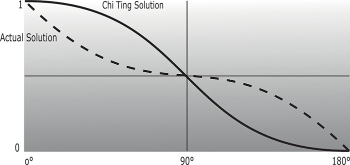
Figure 7.3 Analytic hemisphere lighting function
Compares the actual analytic function for hemisphere lighting to a similar but higher-performance function.
For the hemisphere shader, we need to pass in uniform variables for the sky color and the ground color. We can also consider the “north pole” to be our light position. If we pass this in as a uniform variable, we can light the model from different directions.
Example 7.12 shows a vertex shader that implements hemisphere lighting. As you can see, the shader is quite simple. The main purpose of the shader is to compute the diffuse color value and leave it in the user-defined out variable Color, as with the chapter’s earlier examples. Results for this shader are shown in Figure 7.4. Compare the hemisphere lighting (D) with a single directional light source (A and B). Not only is the hemisphere shader simpler and more efficient, but it produces a much more realistic lighting effect too! This lighting model can be utilized for tasks like model preview, where it is important to examine all the details of a model. It can also be used in conjunction with the traditional computer graphics illumination model. Point lights, directional lights, or spotlights can be added on top of the hemisphere lighting model to provide more illumination to important parts of the scene. And, as always, if you want to move some or all these computations to the fragment shader, you may do so.

Figure 7.4 Lighting model comparison
A comparison of some of the lighting models discussed in this chapter. The model uses a base color of white, RGB = (1.0, 1.0, 1.0), to emphasize areas of light and shadow. (A) uses a directional light above and to the right of the model. (B) uses a directional light directly above the model. These two images illustrate the difficulties with the traditional lighting model. Detail is lost in areas of shadow. (D) illustrates hemisphere lighting. (E) illustrates spherical harmonic lighting using the Old Town Square coefficients. (3Dlabs, Inc.)
Example 7.12 Vertex Shader for Hemisphere Lighting
#version 330 core
uniform vec3 LightPosition;
uniform vec3 SkyColor;
uniform vec3 GroundColor;
uniform mat4 MVMatrix;
uniform mat4 MVPMatrix;
uniform mat3 NormalMatrix;
in vec4 VertexPosition;
in vec3 VertexNormal;
out vec3 Color;
void main()
{
vec3 position = vec3(MVMatrix * VertexPosition);
vec3 tnorm = normalize(NormalMatrix * VertexNormal);
vec3 lightVec = normalize(LightPosition - position);
float costheta = dot(tnorm, lightVec);
float a = costheta * 0.5 + 0.5;
Color = mix(GroundColor, SkyColor, a);
gl_Position = MVPMatrix * VertexPosition;
}
One of the issues with this model is that it doesn’t account for self-occlusion. Regions that should really be in shadow because of the geometry of the model will appear too bright. We remedy this later.
Image-Based Lighting
If we’re trying to achieve realistic lighting in a computer graphics scene, why not just use an environment map for the lighting? This approach to illumination is called image-based lighting; it has been popularized in recent years by researcher Paul Debevec at the University of Southern California. Churches and auditoriums may have dozens of light sources on the ceiling. Rooms with many windows also have complex lighting environments. It is often easier and much more efficient to sample the lighting in such environments and store the results in one or more environment maps than it is to simulate numerous individual light sources. The steps involved in image-based lighting are as follows:
1. Use a light probe (e.g., a reflective sphere) to capture (e.g., photograph) the illumination that occurs in a real-world scene. The captured omnidirectional, high-dynamic-range image is called a light-probe image.
2. Use the light-probe image to create a representation of the environment (e.g., an environment map).
3. Place the synthetic objects to be rendered inside the environment.
4. Render the synthetic objects by using the representation of the environment created in Step 2.
On his Web site (www.pauldebevec.org), Debevec offers a number of useful things to developers. For one, he has made available a number of images that can be used as high-quality environment maps to provide realistic lighting in a scene. These images are high-dynamic-range (HDR) images that represent each color component with a 32-bit floating-point value. Such images can represent a much greater range of intensity values than can 8-bit-per-component images. For another, he makes available a tool called HDRShop that manipulates and transforms these environment maps. Through links to his various publications and tutorials, he also provides step-by-step instructions on creating your own environment maps and using them to add realistic lighting effects to computer-graphics scenes.
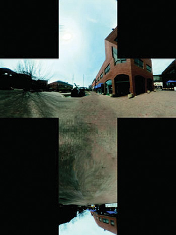
Following Debevec’s guidance, we purchased a 2-inch chrome steel ball from McMaster-Carr Supply Company (www.mcmaster.com). We used this ball to capture a light-probe image from the center of the square outside our office building in downtown Fort Collins, Colorado, shown in Figure 7.5. We then used HDRShop to create a lat-long environment map, shown in Figure 7.6, and a cube map, shown in Figure 7.7. The cube map and latlong map can be used to perform environment mapping. That shader simulated a surface with an underlying base color and diffuse reflection characteristics that was covered by a transparent mirrorlike layer that reflected the environment flawlessly.
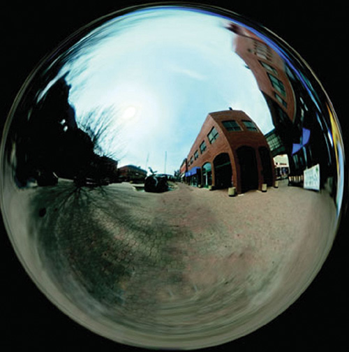
Figure 7.5 Light probe image
A light-probe image of Old Town Square, Fort Collins, Colorado (3Dlabs, Inc.)
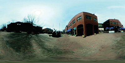
Figure 7.6 Lat-long map
An equirectangular (or lat-long) texture map of Old Town Square, Fort Collins, Colorado (3Dlabs, Inc.)
We can simulate other types of objects if we modify the environment maps before they are used. A point on the surface that reflects light in a diffuse fashion reflects light from all the light sources that are in the hemisphere in the direction of the surface normal at that point. We can’t really afford to access the environment map a large number of times in our shader. What we can do instead is similar to what we discussed for hemisphere lighting. Starting from our light-probe image, we can construct an environment map for diffuse lighting. Each texel in this environment map will contain the weighted average (i.e., the convolution) of other texels in the visible hemisphere as defined by the surface normal that would be used to access that texel in the environment.
Again, HDRShop has exactly what we need. We can use HDRShop to create a lat-long image from our original light-probe image. We can then use a command built into HDRShop that performs the necessary convolution.
This operation can be time consuming, because at each texel in the image, the contributions from half of the other texels in the image must be considered. Luckily, we don’t need a very large image for this purpose. The effect is essentially the same as creating a very blurry image of the original light-probe image. Because there is no high-frequency content in the computed image, a cube map with faces that are 64 × 64 or 128 × 128 works just fine.
A single texture access into this diffuse environment map provides us with the value needed for our diffuse reflection calculation. What about the specular contribution? A surface that is very shiny will reflect the illumination from a light source, just like a mirror. A single point on the surface reflects a single point in the environment. For surfaces that are rougher, the highlight defocuses and spreads out. In this case, a single point on the surface reflects several points in the environment, though not the whole visible hemisphere, like a diffuse surface. HDRShop lets us blur an environment map by providing a Phong exponent—a degree of shininess. A value of 1.0 convolves the environment map to simulate diffuse reflection, and a value of 50 or more convolves the environment map to simulate a somewhat shiny surface.
The shaders that implement these concepts end up being quite simple and quite fast. In the vertex shader, all that is needed is to compute the reflection direction at each vertex. This value and the surface normal are sent to the fragment shader as out variables. They are interpolated across each polygon, and the interpolated values are used in the fragment shader to access the two environment maps in order to obtain the diffuse and the specular components. The values obtained from the environment maps are combined with the object’s base color to arrive at the final color for the fragment. The shaders are shown in Example 7.13. Examples of images created with this technique are shown in Figure 7.8.
Figure 7.8 Effects of diffuse and specular environment maps
This variety of effects uses the Old Town Square diffuse and specular environment maps shown in Figure 7.6. Left: BaseColor set to (1.0, 1.0, 1.0), SpecularPercent is 0, and DiffusePercent is 1.0. Middle: BaseColor is set to (0, 0, 0), SpecularPercent is set to 1.0, and DiffusePercent is set to 0. Right: BaseColor is set to (0.35, 0.29, 0.09), SpecularPercent is set to 0.75, and DiffusePercent is set to 0.5. (3Dlabs, Inc.)
Example 7.13 Shaders for Image-Based Lighting
--------------------------- Vertex Shader -----------------------------
// Vertex shader for image-based lighting
#version 330 core
uniform mat4 MVMatrix;
uniform mat4 MVPMatrix;
uniform mat3 NormalMatrix;
in vec4 VertexPosition;
in vec3 VertexNormal;
out vec3 ReflectDir;
out vec3 Normal;
void main()
{
Normal = normalize(NormalMatrix * VertexNormal);
vec4 pos = MVMatrix * VertexPosition;
vec3 eyeDir = pos.xyz;
ReflectDir = reflect(eyeDir, Normal);
gl_Position = MVPMatrix * VertexPosition;
}
-------------------------- Fragment Shader ----------------------------
// Fragment shader for image-based lighting
#version 330 core
uniform vec3 BaseColor;
uniform float SpecularPercent;
uniform float DiffusePercent;
uniform samplerCube SpecularEnvMap;
uniform samplerCube DiffuseEnvMap;
in vec3 ReflectDir;
in vec3 Normal;
out vec4 FragColor;
void main()
{
// Look up environment map values in cube maps
vec3 diffuseColor =
vec3(texture(DiffuseEnvMap, normalize(Normal)));
vec3 specularColor =
vec3(texture(SpecularEnvMap, normalize(ReflectDir)));
// Add lighting to base color and mix
vec3 color = mix(BaseColor, diffuseColor*BaseColor, DiffusePercent);
color = mix(color, specularColor + color, SpecularPercent);
FragColor = vec4(color, 1.0);
}
The environment maps that are used can reproduce the light from the whole scene. Of course, objects with different specular reflection properties require different specular environment maps. And producing these environment maps requires some manual effort and lengthy preprocessing. But the resulting quality and performance make image-based lighting a great choice in many situations.
Lighting with Spherical Harmonics
In 2001, Ravi Ramamoorthi and Pat Hanrahan presented a method that uses spherical harmonics for computing the diffuse lighting term. This method reproduces accurate diffuse reflection, based on the content of a light-probe image, without accessing the light-probe image at runtime. The light-probe image is preprocessed to produce coefficients that are used in a mathematical representation of the image at runtime. The mathematics behind this approach is beyond the scope of this book. Instead, we lay the necessary groundwork for this shader by describing the underlying mathematics in an intuitive fashion. The result is remarkably simple, accurate, and realistic, and it can easily be codified in an OpenGL shader. This technique has already been used successfully to provide real-time illumination for games and has applications in computer vision and other areas as well.
Spherical harmonics provides a frequency-space representation of an image over a sphere. It is analogous to the Fourier transform on the line or circle. This representation of the image is continuous and rotationally invariant. Using this representation for a light-probe image, Ramamoorthi and Hanrahan showed that you could accurately reproduce the diffuse reflection from a surface with just nine spherical harmonic basis functions. These nine spherical harmonics are obtained with constant, linear, and quadratic polynomials of the normalized surface normal.
Intuitively, we can see that it is plausible to accurately simulate the diffuse reflection with a small number of basis functions in frequency space because diffuse reflection varies slowly across a surface. With just nine terms used, the average error over all surface orientations is less than 3 percent for any physical input lighting distribution. With Debevec’s light-probe images, the average error was shown to be less than 1 percent, and the maximum error for any pixel was less than 5 percent.
Each spherical harmonic basis function has a coefficient that depends on the light-probe image being used. The coefficients are different for each color channel, so you can think of each coefficient as an RGB value. A preprocessing step is required to compute the nine RGB coefficients for the light-probe image to be used. Ramamoorthi makes the code for this preprocessing step available for free on his Web site. We used this program to compute the coefficients for all the light-probe images in Debevec’s light-probe gallery as well as the Old Town Square light-probe image and summarized the results in Table 7.1.

The formula for diffuse reflection using spherical harmonics is

The constants c1–c5 result from the derivation of this formula and are shown in the vertex shader code in Example 7.14. The L coefficients are the nine basis function coefficients computed for a specific light-probe image in the preprocessing phase. The x, y, and z values are the coordinates of the normalized surface normal at the point that is to be shaded. Unlike low-dynamic-range (LDR) images (e.g., 8 bits per color component) that have an implicit minimum value of 0 and an implicit maximum value of 255, HDR images represented with a floating-point value for each color component don’t contain well-defined minimum and maximum values. The minimum and maximum values for two HDR images may be quite different unless the same calibration or creation process was used to create both images. It is even possible to have an HDR image that contains negative values. For this reason, the vertex shader contains an overall scaling factor to make the final effect look right.
The vertex shader that encodes the formula for the nine spherical harmonic basis functions is actually quite simple. When the compiler gets hold of it, it becomes simpler still. An optimizing compiler typically reduces all the operations involving constants. The resulting code is quite efficient because it contains a relatively small number of addition and multiplication operations that involve the components of the surface normal.
Example 7.14 Shaders for Spherical Harmonics Lighting
--------------------------- Vertex Shader -----------------------------
// Vertex shader for computing spherical harmonics
#version 330 core
uniform mat4 MVMatrix;
uniform mat4 MVPMatrix;
uniform mat3 NormalMatrix;
uniform float ScaleFactor;
const float C1 = 0.429043;
const float C2 = 0.511664;
const float C3 = 0.743125;
const float C4 = 0.886227;
const float C5 = 0.247708;
// Constants for Old Town Square lighting
const vec3 L00 = vec3( 0.871297, 0.875222, 0.864470);
const vec3 L1m1 = vec3( 0.175058, 0.245335, 0.312891);
const vec3 L10 = vec3( 0.034675, 0.036107, 0.037362);
const vec3 L11 = vec3(-0.004629, -0.029448, -0.048028);
const vec3 L2m2 = vec3(-0.120535, -0.121160, -0.117507);
const vec3 L2m1 = vec3( 0.003242, 0.003624, 0.007511);
const vec3 L20 = vec3(-0.028667, -0.024926, -0.020998);
const vec3 L21 = vec3(-0.077539, -0.086325, -0.091591);
const vec3 L22 = vec3(-0.161784, -0.191783, -0.219152);
in vec4 VertexPosition;
in vec3 VertexNormal;
out vec3 DiffuseColor;
void main()
{
vec3 tnorm = normalize(NormalMatrix * VertexNormal);
DiffuseColor = C1 * L22 * (tnorm.x * tnorm.x - tnorm.y * tnorm.y) +
C3 * L20 * tnorm.z * tnorm.z +
C4 * L00 -
C5 * L20 +
2.0 * C1 * L2m2 * tnorm.x * tnorm.y +
2.0 * C1 * L21 * tnorm.x * tnorm.z +
2.0 * C1 * L2m1 * tnorm.y * tnorm.z +
2.0 * C2 * L11 * tnorm.x +
2.0 * C2 * L1m1 * tnorm.y +
2.0 * C2 * L10 * tnorm.z;
DiffuseColor *= ScaleFactor;
gl_Position = MVPMatrix * VertexPosition;
}
-------------------------- Fragment Shader ----------------------------
// Fragment shader for lighting with spherical harmonics
#version 330 core
in vec3 DiffuseColor;
out vec4 FragColor;
void main()
{
FragColor = vec4(DiffuseColor, 1.0);
}
Our fragment shader, shown in Example 7.14, has very little work to do. Because the diffuse reflection typically changes slowly, for scenes without large polygons we can reasonably compute it in the vertex shader and interpolate it during rasterization. As with hemispherical lighting, we can add procedurally defined point lights, directional lights, or spotlights on top of the spherical harmonics lighting to provide more illumination to important parts of the scene. Results of the spherical harmonics shader are shown in Figure 7.9. We could make the diffuse lighting from the spherical harmonics computation more subtle by blending it with the object’s base color.
Figure 7.9 Spherical harmonics lighting
Lighting using the coefficients from Table 7.1. From the left: Old Town Square, Grace Cathedral, Galileo’s Tomb, Campus Sunset, and St. Peter’s Basilica. (3Dlabs, Inc.)
The trade-offs in using image-based lighting versus procedurally defined lights are similar to the trade-offs between using stored textures versus procedural textures. Image-based lighting techniques can capture and re-create complex lighting environments relatively easily. It would be exceedingly difficult to simulate such an environment with a large number of procedural light sources. On the other hand, procedurally defined light sources do not use up texture memory and can easily be modified and animated.
Shadow Mapping
Recent advances in computer graphics have produced a plethora of techniques for rendering realistic lighting and shadows. OpenGL can be used to implement almost any of them. In this section, we will cover one technique known as shadow mapping, which uses a depth texture to determine whether a point is lit or not.
Shadow mapping is a multipass technique that uses depth textures to provide a solution to rendering shadows. A key pass is to view the scene from the shadow-casting light source rather than from the final viewpoint. By moving the viewpoint to the position of the light source, you will notice that everything seen from that location is lit; there are no shadows from the perspective of the light. By rendering the scene’s depth from the point of view of the light into a depth buffer, we can obtain a map of the shadowed and unshadowed points in the scene; a shadow map. Those points visible to the light will be rendered, and those points hidden from the light (those in shadow) will be culled away by the depth test. The resulting depth buffer then contains the distance from the light to the closest point to the light for each pixel. It contains nothing for anything in shadow.
The condensed two-pass description is as follows:
• Render the scene from the point of view of the light source. It doesn’t matter what the scene looks like; you want only the depth values. Create a shadow map by attaching a depth texture to a framebuffer object and rendering depth directly into it.
• Render the scene from the point of view of the viewer. Project the surface coordinates into the light’s reference frame and compare their depths to the depth recorded into the light’s depth texture. Fragments that are farther from the light than the recorded depth value are not visible to the light and, hence, in shadow.
The following sections provide a more detailed discussion, along with sample code illustrating each of the steps.
Creating a Shadow Map
The first step is to create a texture map of depth values as seen from the light’s point of view. You create this by rendering the scene with the viewpoint located at the light’s position. Before we can render depth into a depth texture, we need to create the depth texture and attach it to a framebuffer object. Example 7.15 shows how to do this. This code is included in the initialization sequence for the application.
Example 7.15 Creating a Framebuffer Object with a Depth Attachment
// Create a depth texture
glGenTextures(1, &depth_texture);
glBindTexture(GL_TEXTURE_2D, depth_texture);
// Allocate storage for the texture data
glTexImage2D(GL_TEXTURE_2D, 0, GL_DEPTH_COMPONENT32,
DEPTH_TEXTURE_SIZE, DEPTH_TEXTURE_SIZE,
0, GL_DEPTH_COMPONENT, GL_FLOAT, NULL);
// Set the default filtering modes
glTexParameteri(GL_TEXTURE_2D, GL_TEXTURE_MIN_FILTER, GL_LINEAR);
glTexParameteri(GL_TEXTURE_2D, GL_TEXTURE_MAG_FILTER, GL_LINEAR);
// Set up depth comparison mode
glTexParameteri(GL_TEXTURE_2D, GL_TEXTURE_COMPARE_MODE,
GL_COMPARE_REF_TO_TEXTURE);
glTexParameteri(GL_TEXTURE_2D, GL_TEXTURE_COMPARE_FUNC, GL_LEQUAL);
// Set up wrapping modes
glTexParameteri(GL_TEXTURE_2D, GL_TEXTURE_WRAP_S, GL_CLAMP_TO_EDGE);
glTexParameteri(GL_TEXTURE_2D, GL_TEXTURE_WRAP_T, GL_CLAMP_TO_EDGE);
glBindTexture(GL_TEXTURE_2D, 0);
// Create FBO to render depth into
glGenFramebuffers(1, &depth_fbo);
glBindFramebuffer(GL_FRAMEBUFFER, depth_fbo);
// Attach the depth texture to it
glFramebufferTexture(GL_FRAMEBUFFER, GL_DEPTH_STENCIL_ATTACHMENT,
depth_texture, 0);
// Disable color rendering as there are no color attachments
glDrawBuffer(GL_NONE);
In Example 7.15, the depth texture is created and allocated using the GL_DEPTH_COMPONENT32 internal format. This creates a texture that is capable of being used as the depth buffer for rendering and as a texture that can be used later for reading from. Notice also how we set the texture comparison mode. This allows us to leverage shadow textures—a feature of OpenGL that allows the comparison between a reference value and a value stored in the texture to be performed by the texture hardware rather than explicitly in the shader. In the example, DEPTH_TEXTURE_SIZE has previously been defined to be the desired size for the shadow map. This should generally be at least as big as the default framebuffer (your OpenGL window); otherwise, aliasing and sampling artifacts could be present in the resulting images. However, making the depth texture unnecessarily large will waste lots of memory and bandwidth and adversely affect the performance of your program.
The next step is to render the scene from the point of view of the light. To do this, we create a view-transformation matrix for the light source, using the provided lookat function. We also need to set the light’s projection matrix. As world and eye coordinates for the light’s viewpoint, we can multiply these matrices together to provide a single view-projection matrix. In this simple example we can also bake the scene’s model matrix into the same matrix (providing a model-view-projection matrix to the light shader). The code to perform these steps is shown in Example 7.16.
Example 7.16 Setting up the Matrices for Shadow-Map Generation
// Time varying light position
vec3 light_position = vec3(sinf(t * 6.0f * 3.141592f) * 300.0f,
200.0f,
cosf(t * 4.0f * 3.141592f) * 100.0f + 250.0f);
// Matrices for rendering the scene
mat4 scene_model_matrix = rotate(t * 720.0f, Y);
// Matrices used when rendering from the light's position
mat4 light_view_matrix = lookat(light_position, vec3(0.0f), Y);
mat4 light_projection_matrix(frustum(-1.0f, 1.0f, -1.0f, 1.0f,
1.0f, FRUSTUM_DEPTH));
// Now we render from the light's position into the depth buffer.
// Select the appropriate program
glUseProgram(render_light_prog);
glUniformMatrix4fv(render_light_uniforms.MVPMatrix,
1, GL_FALSE,
light_projection_matrix *
light_view_matrix *
scene_model_matrix);
In Example 7.16, we set the light’s position using a function of time (t) and point it toward the origin. This will cause the shadows to move around. FRUSTUM_DEPTH is set to the maximum depth over which the light will influence and represents the far plan of the light’s frustum. The near plane is set to 1.0f, but ideally, the ratio of far-plane to near-plane distance should be as small as possible (i.e., the near plane should be as far as possible from the light, and the far plane should be as close as possible to the light) to maximize the precision of the depth buffer.
The shaders used to generate the depth buffer from the light’s position are trivial. The vertex shader simply transforms the incoming position by the provided model-view-projection matrix. The fragment shader writes a constant into a dummy output and is present only because OpenGL requires it.1 The vertex and fragment shaders used to render depth from the light’s point of view are shown in Example 7.17.
1. The results of rasterization are undefined in OpenGL if no fragment shader is present. It is legal to have no fragment shader when rasterization is turned off, but here, we do want to rasterize so that we can generate depth values for the scene.
Example 7.17 Simple Shader for Shadow-Map Generation
--------------------------- Vertex Shader -----------------------------
// Vertex shader for shadow-map generation
#version 330 core
uniform mat4 MVPMatrix;
layout (location = 0) in vec4 position;
void main(void)
{
gl_Position = MVPMatrix * position;
}
-------------------------- Fragment Shader ----------------------------
// Fragment shader for shadow-map generation
#version 330 core
layout (location = 0) out vec4 color;
void main(void)
{
color = vec4(1.0);
}
At this point, we are ready to render the scene into the depth texture we created earlier. We need to bind the framebuffer object with the depth texture attachment and set the viewport to the depth texture size. Then we clear the depth buffer (which is actually our depth texture now) and draw the scene. Example 7.18 contains the code to do this.
Example 7.18 Rendering the Scene from the Light’s Point of View
// Bind the 'depth only' FBO and set the viewport
// to the size of the depth texture
glBindFramebuffer(GL_FRAMEBUFFER, depth_fbo);
glViewport(0, 0, DEPTH_TEXTURE_SIZE, DEPTH_TEXTURE_SIZE);
// Clear
glClearDepth(1.0f);
glClear(GL_DEPTH_BUFFER_BIT);
// Enable polygon offset to resolve depth-fighting issues
glEnable(GL_POLYGON_OFFSET_FILL);
glPolygonOffset(2.0f, 4.0f);
// Draw from the light's point of view
DrawScene(true);
glDisable(GL_POLYGON_OFFSET_FILL);
Notice that we’re using polygon offset here. This pushes the generated depth values away from the viewer (the light, in this case) by a small amount. In this application, we want the depth test to be conservative, insofar as when there is doubt about whether a point is in shadow or not, we want to light it. If we did not do this, we would end up with depth fighting in the rendered image due to precision issues with the floating-point depth buffer. Figure 7.10 shows the resulting depth map of our scene as seen from the light’s position.

Figure 7.10 Depth rendering
Depths are rendered from the light’s position. Within rendered objects, closer points have smaller depths and show up darker.
Using a Shadow Map
Now that we have the depth for the scene rendered from the light’s point of view, we can render the scene with our regular shaders and use the resulting depth texture to produce shadows as part of our lighting calculations. This is where the meat of the algorithm is. First, we need to set up the matrices for rendering the scene from the viewer’s position. The matrices we need are the model matrix, view matrix (which transforms vertices for classic lighting), and projection matrix (which transforms coordinates to projective space for rasterization). Also, we need a shadow matrix. This matrix transforms world coordinates into the light’s projective space and simultaneously applies a scale and bias to the resulting depth values. The transformation to the light’s eye space is performed by transforming the world space vertex coordinates through the light’s view matrix followed by the light’s projection matrix (which we calculated earlier). The scale and bias matrix maps depth values in projection space (which lie between –1.0 and +1.0) into the range 0.0 to 1.0.
The code to set all these matrices up is given in Example 7.19.
Example 7.19 Matrix Calculations for Shadow-Map Rendering
mat4 scene_model_matrix = rotate(t * 720.0f, Y);
mat4 scene_view_matrix = translate(0.0f, 0.0f, -300.0f);
mat4 scene_projection_matrix = frustum(-1.0f, 1.0f, -aspect, aspect,
1.0f, FRUSTUM_DEPTH);
mat4 scale_bias_matrix = mat4(vec4(0.5f, 0.0f, 0.0f, 0.0f),
vec4(0.0f, 0.5f, 0.0f, 0.0f),
vec4(0.0f, 0.0f, 0.5f, 0.0f),
vec4(0.5f, 0.5f, 0.5f, 1.0f));
mat4 shadow_matrix = scale_bias_matrix *
light_projection_matrix *
light_view_matrix;
The vertex shader used for the final render transforms the incoming vertex coordinates through all of these matrices and provides world coordinates, eye coordinates, and shadow coordinates to the fragment shader, which will perform the actual lighting calculations. This vertex shader is given in Example 7.20.
Example 7.20 Vertex Shader for Rendering from Shadow Maps
#version 330 core
uniform mat4 model_matrix;
uniform mat4 view_matrix;
uniform mat4 projection_matrix;
uniform mat4 shadow_matrix;
layout (location = 0) in vec4 position;
layout (location = 1) in vec3 normal;
out VS_FS_INTERFACE
{
vec4 shadow_coord;
vec3 world_coord;
vec3 eye_coord;
vec3 normal;
} vertex;
void main(void)
{
vec4 world_pos = model_matrix * position;
vec4 eye_pos = view_matrix * world_pos;
vec4 clip_pos = projection_matrix * eye_pos;
vertex.world_coord = world_pos.xyz;
vertex.eye_coord = eye_pos.xyz;
vertex.shadow_coord = shadow_matrix * world_pos;
vertex.normal = mat3(view_matrix * model_matrix) * normal;
gl_Position = clip_pos;
}
Finally, the fragment shader performs lighting calculations for the scene. If the point is considered to be illuminated by the light, the light’s contribution is included in the final lighting calculation; otherwise, only ambient light is applied. The shader given in Example 7.21 performs these calculations.
Example 7.21 Fragment Shader for Rendering from Shadow Maps
#version 330 core
uniform sampler2DShadow depth_texture;
uniform vec3 light_position;
uniform vec3 material_ambient;
uniform vec3 material_diffuse;
uniform vec3 material_specular;
uniform float material_specular_power;
layout (location = 0) out vec4 color;
in VS_FS_INTERFACE
{
vec4 shadow_coord;
vec3 world_coord;
vec3 eye_coord;
vec3 normal;
} fragment;
void main(void)
{
vec3 N = fragment.normal;
vec3 L = normalize(light_position - fragment.world_coord);
vec3 R = reflect(-L, N);
vec3 E = normalize(fragment.eye_coord);
float NdotL = dot(N, L);
float EdotR = dot(-E, R);
float diffuse = max(NdotL, 0.0);
float specular = max(pow(EdotR, material_specular_power), 0.0);
float f = textureProj(depth_texture, fragment.shadow_coord);
color = vec4(material_ambient +
f * (material_diffuse * diffuse +
material_specular * specular), 1.0);
}
Don’t worry about the complexity of the lighting calculations in this shader. The important part of the algorithm is the use of the sampler2DShadow sampler type and the textureProj function. The sampler2DShadow sampler is a special type of 2D texture that, when sampled, will return 1.0 if the sampled texture satisfies the comparison test for the texture or 0.0 if it does not. The texture comparison mode for the depth texture was set earlier in Example 7.15 by calling glTextureParameteri() with the GL_TEXTURE_COMPARE_MODE parameter name and GL_COMPARE_REF_TO_TEXTURE parameter value. When the depth comparison mode for the texture is configured like this, the texel values will be compared against the reference value that is supplied in the third component of fragment.shadow_coord—which is the z component of the scaled and biased projective-space coordinate of the fragment as viewed from the light. The depth comparison function is set to GL_LEQUAL, which causes the test to pass if the reference value is less than or equal to the value in the texture. When multiple texels are sampled (e.g., when the texture mode is linear), the result of reading from the texture is the average of all the 0.0s and 1.0s for the samples making up the final texel. That is, near the edge of a shadow, the returned value might be 0.25, or 0.5, and so on, rather than just 0.0 or 1.0. We scale the lighting calculations by this result to take light visibility into account during shading.
The textureProj function is a projective texturing function. It divides the incoming texture coordinate (in this case fragment.shadow_coord by its own last component (fragment.shadow_coord.w) to transform it into normalized device coordinates, which is exactly what the perspective transformation performed by OpenGL before rasterization does.
The result of rendering our scene with this shader is shown in Figure 7.11.
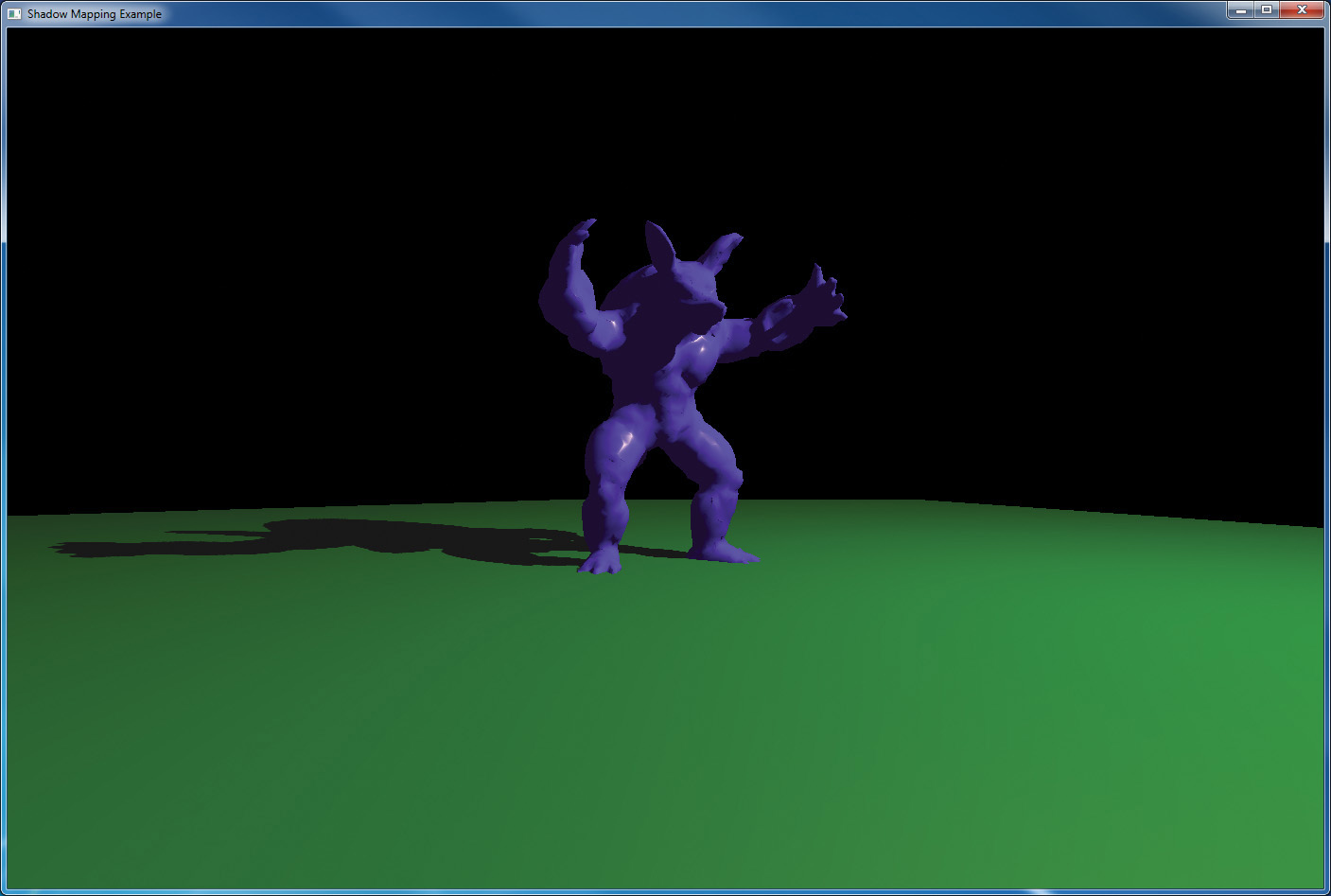
That wraps up shadow mapping. There are many other techniques, including enhancements to shadow mapping, and we encourage you to explore them on your own.