Chapter 16

Responding to Risks That Threaten Your Project

In This Chapter

Monitoring the progress of a project

Using risk registers to plan ahead

Reacting to risk in a positive way

Responding to risk in the cost, quality, scope, and especially timing of your project can only be done well if you can identify and prepare for those risks beforehand. Trying to correct for those risks without preparation delays your response time, letting things only get more out of control as you try to develop response plans on the fly. One of the marks of a superb project manager is his ability to anticipate, plan for, and successfully manage project risks.

In this chapter, we explore the two key tools needed to manage risk effectively. One is a good tracking system so that you know whether your project is on schedule and budget. In practice, this is trickier than it sounds. However, there are some common methods that work well.

The other main tool is a structured approach to identifying and preparing for risk ahead of time. By identifying cost, quality, scope, and especially timing risks ahead of time, sometimes you can eliminate them entirely at the beginning of the project at relatively low cost. For other risks, you may take a wait-and-see approach. However, if the worst does happen, having a contingency plan in place can make the difference between successfully coping with a problem and having that problem sink your project.

Finally, sometimes you fall behind despite your best efforts to anticipate and manage obstacles. What do you do? The answers are not intuitive. For example, adding lots of extra employees often can sink your project because the resources you need to get them up to speed must be stolen from completing the project. We finish the chapter by discussing these problems and how best to cope with them.

Tracking Project Progress

One of the major causes of project failure is poor tracking of project progress. The reason for this is that it’s almost always easier and more effective to make corrective actions earlier rather than later in a project’s execution. If you can’t or don’t track project progress on an ongoing basis, you’re going to find out you’re in trouble far too late to do anything effective. To avoid this, project managers have a number of options to track progress effectively.

Assessing earned value

There are a number of ways to track project progress. One of the simplest is to set up milestones during the project planning phase of the project life cycle (see Chapter 14). If there are enough milestones and they are spaced relatively evenly, you can get a good idea of where you are in the project by tracking which milestones have been completed on a regular basis.

A more sophisticated method is the earned value (EV) analysis approach. To use this approach, list all the activities in your project, along with their estimated costs. (Find out how to estimate costs in Chapter 15.)

Figure 16-1 shows an example of earned value analysis tracking at the end of week 8 for an example project. To perform the analysis, find these four metrics for each activity:

Budgeted cost: In the planning phase of the project, determine how much it will cost to complete each activity. For activity B in Figure 16-1, the budgeted cost is $2,000. For activity D, it’s $6,000. These values don’t change over time.

Planned value: This is estimated from the planning phase upfront about how much you’ll spend on completing an activity. During the planning phase of the project depicted in Figure 16-1, activity B was expected to be complete by the end of week 8. So 100 percent of the budgeted cost of $2,000 yields a “planned value” of $2,000. In contrast, activity D was planned to be only 30 percent complete by end of week 8, so its planned value is 30 percent of the budgeted cost of $6,000, which yields a planned value of $1,800.

Actual cost: This is what you actually end up spending on completing an activity. In the example, this is $1,900 for activity B and $2,100 for activity D. Usually, the actual cost won’t equal the planned value (although hopefully it’s close).

Earned value: This is the actual percent complete for an activity times its budgeted cost. For activity B in Figure 16-1, 100 percent of the project was actually complete by the end of week 8; 100 percent of the budgeted cost for activity B of $2,000 is $2,000. Thus, though it cost only $1,900 to complete activity B, the earned value for project monitoring purposes is $2,000. Activity D is only actually 25 percent complete at the end of week 8, so its earned value is 25 percent of its budgeted cost of $6,000, or $1,500. Note that activity D’s earned value will increase in subsequent weeks (at least we hope so!).

Illustration by Wiley, Composition Services Graphics

Figure 16-1: Example earned value analysis.

Now you need to find the planned value (PV), actual cost (AC), and earned value (EV) of the entire project. To do this, you’ll figure out what activities you planned to complete by now in the project versus what you actually have completed. You’ll also need to figure out what you planned to spend versus what you actually have spent.

To find the PV for the project described in Figure 16-1, sum up the PVs for all the activities at the end of week 8. This gives you a total of $8,050. Adding up the ACs of all the activities totals $11,000. Finally, summing the EVs totals $8,375 at the end of week 8. This means that the PV is $8,050, the AC $11,000, and the EV is $8,375 for this example project.

Now calculate these four measures of progress for the earned value method:

Cost variance (CV): CV = EV – AC

This is how much less than you’ve spent by this point in the project than what you planned to. It’s measured in dollars. Counterintuitively, a positive variance is good, and a negative variance is bad.

Schedule variance (SV): SV = EV – PV

This is how much more of the project you’ve completed by this point in the project than you planned to. It’s measured in dollars. Again, a positive variance is good; a negative variance is bad.

Cost performance index (CPI): EV/AC

This is the ratio of how much you’ve spent on the project by this point over what you had planned to. It’s measured as a percentage. Counterintuitively, a value above 100 percent is good, and a value below 100 percent is bad.

Schedule performance index (SPI): EV/PV

This is the ratio of how much of the project you’ve completed by this point over what you had planned to. It’s measured as a percentage. A value above 100 percent is good, and a value below 100 percent is bad.

In all four of these measures, higher is better. For example, a cost performance index (CPI) of 110 percent means that the project is not 10 percent over budget, but 9.09 percent under budget (1 – 1/1.10 = 0.909).

The example described in Figure 16-1 has these tracking measures:

Cost variance is EV – AC = $8,375 – $11,000 = –$2,625. This means the project is $2,625 over budget at the end of week 8. Yes, negative does mean it’s over budget. A positive value would actually be under budget.

Schedule variance is EV – PV = $8,375 – $8,050 = $325. So the project is $325 ahead of schedule at the end of week 8. (Yes, this method does use dollars to measure time!)

Cost performance index is EV/AC = $8,375/$11,000 = 76.1 percent. This means the project is significantly over budget. (1/0.761 – 1 = 31.3 percent over budget, to be precise.) Frankly, for project management purposes, saying that the project is about 100 percent – 76 percent = 34 percent over budget is close enough.

Schedule performance index is EV/PV = $8,375/$8,050 = 104 percent, which means that you are 4 percent ahead of schedule at the end of week 8.

Based on this earned value analysis, your project at week 8 is a little ahead of schedule. Unfortunately, it is way over budget.

Earning value over time

It is common to graph the three values, planned value, actual cost, and earned value for a project over time. However, they are all typically divided by the budgeted cost for the entire project to form percentages as shown in Figure 16-2. For example, if you have an actual cost (AC) of $2.5 million in December 2012, you would divide it by the total budgeted cost for the project (at the planned time of completion) of $3.3 million to get 76 percent. This is what you would graph on the project progress chart in Figure 16.2.

Looking at the chart in Figure 16-2, you can deduce three things rather quickly:

The earned value is lagging the planned value, which means that the project is behind schedule.

The other is that the actual cost is significantly ahead of the earned value. This means that the project is seriously over budget. Note that you don’t want to compare the actual cost to the planned value. If you do, the project looks over budget, but it doesn’t seem nearly as over budget as it really is, because the planned value assumes that you have completed more work than you actually have!

These variances are not improving over time. If anything, they appear to be getting slightly worse. So unless some intervention occurs, the project is going to be late and very over budget.

Illustration by Wiley, Composition Services Graphics

Figure 16-2: Project progress chart.

Finally, the S-shapes of the curves in Figure 16-2 are typical. In fact, any shape other than an at least approximately S-shaped curve is a hint that there may be something wrong with your either your planning or your calculations.

Sometimes, project managers and their clients simplify reporting earned value progress by using one of these approaches:

The 0/100 rule: Counting an activity for purposes of earned value only when it’s 100 percent complete (0–100 method). Otherwise, it is considered 0 percent complete. For example, an activity with a budgeted cost of $800,000 that’s 75 percent complete would have an earned value of $0 (zip, nada, nothing!). This method is typically used for short duration tasks, less than a month.

The 0/50/100 rule: If an activity is between 0 and 49 percent complete, its earned value is $0. If an activity is between 50 and 99 percent complete, its earned value is half its budgeted cost. For example, if an activity has a budgeted cost of $2 million and is 88 percent complete, then its earned value is 50 · $2 million = $1 million. If an activity is 100 percent complete, only then does it get 100 percent of its earned value. For example, a $3 million dollar activity that is 100 percent complete has an earned value of $3 million.

The progress per unit method: For activities that consist of performing a number of identical sub-tasks, you divide how many subtasks you’ve completed by the total number of sub-tasks. For example, if an activity for a project is to install 300 wind turbines for a wind farm project, one natural way is to count progress by the number of wind turbines installed. In this case, if 100 of the 300 turbines have been installed, then that activity’s progress would be 100/300 = 33 percent.

The purpose of using these rules is to take some of the subjectivity out of determining progress completion. But a project needs to have a very large number of activities for the 0/100 or the 0/50/100 rules to work well. Otherwise, measuring the project progress becomes too granular. The progress per unit method, on the other hand, can be applied to many different types of projects because it is so easy to calculate.

Monitoring the metrics: Who’s responsible?

Someone must be responsible for tracking project progress. Otherwise, it may not get done. If it’s a small project, you — as the project manager — can do it yourself. On the other hand, if you’re managing a big project, progress monitoring might itself turn into a full-time job. In that case, you’ll need to appoint someone to do this who (1) understands the project’s technical aspects (so he or she can’t be fooled so easily); (2) is extremely detail-oriented; and (3) you trust implicitly. After the project manager, the person who monitors progress has arguably the most important job within the project. Get someone good!

An interesting aspect to consider is that suppliers might be performing some of your activities. If it’s a big activity, you’ll have to pay them for it, and — unless you’re in the charity business — you’ll only want to pay them for what progress they’ve actually made. The problem is: Who determines the progress that a supplier has made? If you do it, the supplier might very well accuse you of underestimating their work. If the supplier reports their own progress, they very well might exaggerate it, even if unintentionally.

There’s no perfect solution to this problem. But one option is to hire a third-party vendor to monitor the progress of suppliers. Just be sure that you and the supplier agree on who is to do the monitoring upfront. The last time you want to argue over a third-party monitor is when you’re already having an argument over progress!

Realizing your project’s in trouble

While it’s nice to know that your project is ahead of schedule and under budget, the actions you’ll take are probably minimal (other than patting everyone on the back!). What you are really concerned about is whether your project is in trouble. What would be even nicer is to figure out whether the project looks like it’s headed in trouble before it actually is!

There are a number of ways to accomplish this kind of foresight. All of them involve visual charts that reveal trends. The earned value progress chart is the most popular option; it is shown in Figure 16-2. Other options are the project run chart and the buffer penetration chart.

Using a project run chart

The next most common way also uses earned value, but also incorporates some of the ideas from a process control chart, as shown in Chapter 13. However, this version, which is called a project run chart, is simpler. As shown in Figure 16-3, the idea is to graph the schedule progress index (SPI) and cost progress index (CPI) over time.

If your CPI and SPI are equal to or greater than 100 percent, you’re in the “green” zone and in good shape. If either your SPI or CPI index falls below 100 percent but remains above 90 percent, you’re in the “yellow” zone and caution is advised. Make sure that you have plans in place in case things get worse, particularly if either index dips below 90 percent.

If either of your indices drops below 90 percent, you are in the “red” zone. Performance is poor, and you probably need to execute any correction plans you have in place. (Hopefully, you made these while you were in the “caution” zone!)

Illustration by Wiley, Composition Services Graphics

Figure 16-3: Project run chart.

The progress of your CPI and SPI is going to have statistical fluctuations, just like everything else in operations management (or in life, if you are in a more philosophical mood). Sometimes things are going to go better, sometimes worse. So just because you are in the yellow zone does not mean that you need to panic. It just means that you should be watchful and be prepared.

Utilizing slack with a buffer penetration chart

Another version of the run chart is used sometimes to watch the progress of the critical path. The critical path contains all those activities that, if delayed, will delay the project as a whole. They have no “slack” in them. See Chapter 15 for more on how to determine the critical path.

The central idea is to establish a project time reserve or “buffer,” which accounts for the fact that there is going to be some statistical variation in completing your project’s critical path, just like for everything else in operations management. (If we sound like a broken record about this, it’s strictly intentional!) The schedule buffer accounts for the fact that — even if your estimates are perfectly correct — at times you are going to be behind schedule. The question is how much of this is normal statistical happenstance and how much means that your project is in trouble.

The typical approach is to establish an expected (mean) time estimate to complete the project and a maximum time estimate that would be expected under normal statistical circumstances. There are a number of ways to do this. One way that works well is to make the P50 estimate (you have a 50 percent chance of equaling or beating this estimate based on your initial planning) the expected time estimate, and to make the P95 (you have a 95 percent chance of equaling or beating this estimate) estimate the maximum time estimate.

For example, your project’s critical path may have a P50 of 8 months and a P95 of 12.5 months. You set these to be expected and maximum estimates. Then, your Buffer = Maximum – Expected = 12.5 months – 8 months = 4.5 months. Each month you determine how many of the critical path activities you have completed. You’ll need to determine the planned completion date of this last critical path activity. Once you have determined that, just subtract it from the time into the project.

In the project depicted in Figure 16-4, the last activity completed in the critical chain during September was supposed to be completed 6.9 months into the project according to plan. However, by September, 9.0 months have elapsed since the beginning of the project. So your buffer penetration is 6.9 months – 9.0 months = –2.1 months of buffer penetration. (For reasons unknown to the authors, the convention has grown to use a – to indicate buffer penetration.) You can see this graphed in Figure 16-4. If instead, you were ahead of schedule on the critical path, the convention is to graph a zero for buffer penetration. For example, in February, the last completed activity of the critical chain was planned to be completed in 2.5 months. Yet two months have elapsed. Because 2.5 months – 2 months = 0.5 months is a positive number, you graph it as having zero buffer penetration.

Illustration by Wiley, Composition Services Graphics

Figure 16-4: Buffer penetration chart.

Otherwise, the buffer penetration chart works like the project run chart for SPI and CPI shown earlier. Green is okay. Yellow means caution. This is when you want to figure out any contingency plans. Red means it’s time to activate these contingency plans.

Planning Ahead with Risk Registers

Identifying the risks that threaten your project and planning early for how you can minimize impacts to your outcomes shortens your actual response time when one of those risks occurs and improves the effectiveness of the response. In some cases, by planning ahead for risks, you may even be able to take actions that prevent certain risks from occurring.

The risk management process is a cycle with four phases (as shown in Figure 16-5): Identify, prioritize, respond, and track. Keep in mind that risk management begins in the planning stage of the project, and it continues through project execution and into the handover phase. In other words, the wheel of the risk management cycle never stops.

Illustration by Wiley, Composition Services Graphics

Figure 16-5: Risk response cycle.

Knowing what can go wrong

The first and possibly most important risk management activity for a project is to brainstorm all the things that can go wrong. Do this during the planning phase — well before you begin actually executing the project. The most common tool for managing risk is a risk register.

To begin developing a risk register, consider the critical assumptions from the original project proposal that will harm the project if they are violated (see Chapter 14 for details). Then put together a cross-functional team of experts and use the project proposal plus any other information your experts have at their disposal to brainstorm an initial list of risks.

Technology: If your project depends on any new technologies, whether these are information, engineering, or service technologies, these may pose significant risk to positive outcomes because they may not work, they may cost more than you expect, or they may take too long to complete. The likelihood of these risks occurring and their potential harm to the project increase if there are multiple technologies that depend on each other.

Financials: If the financial assumptions such as resource or material costs (or possibly cost of capital or inflation rates) are wrong, then core cost estimates for the overall project profitability might be off. For example, labor or important materials may cost more than you expect, which sets up the potential for going over-budget. A different type of financial risk occurs if the project may end up late. Being late can create problems such as contract penalties or — in the case of product development — lost market share. Again, these impact profit assumptions. For international projects, another financial problem is the rate of currency exchange, which fluctuates continuously.

Market demand: If your project involves building a plant or developing a new product or service, the demand for your product may not be as strong as you originally predict. If demand is less than expected, then so too will revenue, again impacting the profitability of the project. Note that there is a bit of overlap with financial risks because late projects may result in less market share if the project is developing a new service or project.

Organizational: The majority of organizational problems are the result of turnover. If there is somebody on your project who is irreplaceable, then establish a backup and a transition plan in case she leaves for greener pastures. Turnover happens, so be sure to plan for it.

Another organizational-based risk to some projects involves opposition to the project from inside a stakeholder organization. Hopefully, you identify roadblocks, or sources of opposition, during your stakeholder analysis process as described in Chapter 14.

Government or legal: The government regulates many kinds of project from new drug development to building bridges. If permission from the government for a project activity is not forthcoming, great harm can be done to the project. For example, the great nightmare for people managing construction projects is running afoul of some government agency or organization or a legal restriction of some kind. The number of projects derailed by environmental concerns is legion. One gas drilling project was delayed because the noise from it interfered with the breeding activities of gray whales 700 miles away.

The second greatest fear of people managing construction projects is upsetting some non-governmental lobby or pressure group, such as environmental advocacy groups, community activists and so on. For project managers in other industries, these problems are not so prevalent, but they are still a problem. For example, the laptop computer lithium battery fires of the early 2000s were a big problem for computer manufacturers.

Safety: No one wants workers to get injured on a project, but every major bridge that’s ever been built has had fatalities. Some industries are inherently less exposed to safety and health risks, but this is a primary area of concern for major construction and industrial projects. That said, at least one videogaming software company was sued successfully by the spouses of their engineers and programmers for overwork-induced stress resulting in heart attacks and the like. (To be fair, said company was alleged to work their employees up to 100 hours per week.) So no project is entirely free of safety concerns.

Prioritizing risks

Risk registers prioritize risks by likelihood of occurring and severity of impact if it does occur. In an ideal world, a project manager has access to a numerical probability of a risk occurring and the expected value (mean) of its impact in terms of cost or timing. Usually, however, this information is not available, so you want to qualitatively rank the likelihood of experiencing the risk from 1 to 5, with 1 representing a “very low” probability to 5 representing a “very high” probability.

The expected impact of the risk is also ranked from 1 (“very low”) to 5 (“very high”). The two numbers are multiplied to create an unmitigated risk score ranging from 1 to 25. You can then use the risk scores to prioritize the risks.

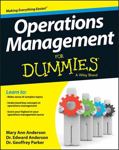
To see this tool in practice, consider an example of the Melville Island tar sands project, whose risk register is shown in Figure 16-6. When oil prices were approximately $125 per barrel, there was some thought given to processing tar sands on Melville Island in Canada for oil. The logistical hurdles would have been immense. The distance to the nearest port, Churchill in Manitoba, Canada, on Hudson Bay, is 1,200 miles. (And Churchill is another 1,100 miles from Winnipeg, but at least there’s a rail link to it.) Melville Island and Hudson Bay are both icebound six months of the year. Finally, there is no permanent human habitation on Melville Island. Any settlement or port would have to be built from scratch with materials sent from Churchill. There is no vegetation except for lichens, moss, and some woody vines that grow along the ground. However, there are a lot of polar bears!

Figure 16-6 shows the risks for a disguised oil exploration company ExploriCo. At the top of the chart is an organizational risk, which is the risk that not enough skilled labor is willing to relocate to Melville Island. (We can’t imagine why. Think of the polar bears romping in your backyard.) The expert group (and again, you should use a group, just like when brainstorming risks) decides that the unmitigated likelihood of this being a problem is medium, so they give it an unmitigated likelihood score of 3 (we’ll get to the mitigated scores in a minute). However, if it does happen: no workers, no project. So they give the risk an unmitigated impact score of 5 (very high). This gives you an unmitigated risk score of 3 · 5 = 15.

Let’s consider another risk, not enough icebreakers available for rent. The risk is that you could lose 6 months of port usability per year. This might very well double the time to complete the project. While the experts think the likelihood score is a 2 (low), the potential impact is a 5 (very high). This creates a risk score for the icebreakers of 2 · 5 = 10.

Illustration by Wiley, Composition Services Graphics

Figure 16-6: Risk register for example Melville Island tar sands project.

You then continue brainstorming risks and assigning them risk scores. This continues until you can’t think of any more risks. However, the identification process does not end with the planning phase. It continues throughout the life cycle of the project until its completion. The risk register is a living document. Likelihood and impact scores change as a project progresses, and new potential risks emerge. All must be continuously tracked.

Developing a contingency plan

After you identify risks, you need to figure out a way to handle them. The best way to handle risks for a given project depends on the nature of the risk and the specifics of the project.

Here are the three basic varieties of risk:

Variance risk: Some risks look like Figure 16-7 in that they have a probabilistic distribution resulting from uncertainties from concerning knowledge, materials, labor productivity, etc. The best way to respond to this type of risk is upfront by doing things like additional research, switching suppliers, and assigning additional resources. Oftentimes, mitigation plans such as using more reliable suppliers may reduce the variance of a risk but increase cost as shown in Figure 16-8. Even so, most project managers prefer the variance risk after response (the dashed line) because it’s more predictable. Because most project managers are risk-averse — they have enough uncertainty in their lives and there is only so much aspirin can do — they prefer to mitigate the risk even if it costs some money.

Contingency risk: Some risks look like Figure 16-9. Here, if a contingency risk occurs, the base cost variance shifts to the right. Sources of contingency risk are things that are predominantly either/or in nature. For example, you either get a building permit, or you don’t. The new battery technology either works, or it doesn’t. Oftentimes, it makes sense to not mitigate a contingency risk upfront, but put in place a contingency plan, should the contingency risk actually occur. One rather drastic contingency plan that sometimes makes sense is simply to terminate the project if the risk occurs.

Illustration by Wiley, Composition Services Graphics

Figure 16-7: Variance risk.

Illustration by Wiley, Composition Services Graphics

Figure 16-8: Response to variance risk.

Illustration by Wiley, Composition Services Graphics

Figure 16-9: Contingency risk.

Unknown unknowns (often referred to as black swans): These are the risks that you know exist but can’t identify. The only way to respond to these risks is to cope with them when you encounter them. One of the goals of the risk identification process in the planning stage is to uncover as many potential black swans as possible so they can be responded to ahead of time.

Black swan risks take their name because, since Roman times, it was proverbial in Europe to refer to something being rare “as a black swan.” As far as Europeans knew, there was no such thing as a black swan because there are no black swans in Europe (or Asia or Africa). However, Dutch Captain Willem de Vlamingh’s explorations around western Australia in 1697 sighted a whole species of — you guessed it — black swans.

Let’s look at the Melville Island example filled out with response plans in Figure 16-10. One risk is “cannot acquire land from the Canadian government.” The experts during the planning phase judged this to have an unmitigated likelihood of 2 (low) but an impact of 5 (very high). This creates an unmitigated risk score of 10.

The policy at ExploriCo is to create response plans for all risks with scores over 5 and particularly for those with risk scores over 10. The mitigation plan the firm comes up with is to treat it upfront by hiring lobbyists to work with the Canadian government to sell the project and allow them to buy up the necessary land rights in Ottawa. Additionally, if the lobbyists don’t succeed, ExploriCo makes a contingency plan to abandon the project early before much money is spent. Importantly, note the mix of upfront and contingency approaches in the response plan.

After they’ve developed the response plan, the experts decide the mitigated likelihood with the response plan in place is a 1 (very low), though the mitigated impact is only reduced slightly to a 4 (high). The resulting risk score is 1 · 4 = 4, which is considered acceptable by ExploriCo.

Illustration by Wiley, Composition Services Graphics

Figure 16-10: Melville Island risk register with contingency risks.

ExploriCo then proceeds with all the other risks with risk scores above 5. It can’t mitigate all risks to a 5 or below through response plans. However, the risk profile of the project is overall much better than prior to the development of response plans.

Response plans, as part of a project’s risk register, need to be continuously tracked and updated over the entire project. As time wears on, some risks can be deleted from the register because they don’t happen and the time period for them to occur passes. Other risks are discovered and need to be added to the register. As this happens, risk management shifts from tracking and identification back to prioritization and response, continuing the risk management cycle until the end of the project.

In any project, opportunities exist as well as risks. Contingency plans for emerging opportunities, if they arise, make it more likely that you can take advantage of them.

Responding Productively to Risk

Responding to risks when they occur is one of the great tests of a project manager. This is particularly complicated by three “laws” that work against efficiently completing the project. One law, Parkinson’s law, applies to times when things are going well. The other two, Brook’s law and Homer’s law, kick you when you’re already down.

Staying productive: Parkinson’s law

Cyril Northcote Parkinson observed in 1955 that “Work expands to fill the time available for its completion.” He based this observation on years of working with the civil service, yet engineers and programmers are often accused of “gold plating” or “over-engineering” (these are both terms meaning that the engineers have developed the project far beyond what the customer requires or cares about) when left with excess time. Yet tightening deadlines too much to prevent “gold-plating” can also be counterproductive. Research consistently shows that employees, when faced with clearly unrealistic deadlines, simply give up trying to meet them and make progress very slowly.

The best approach to avoid Parkinson’s law without driving employees to despair is to establish moderately aggressive timelines.

Recovering from delays: Brook’s law and Homer’s law

When a project falls behind schedule, getting the project back on track is surprisingly difficult. Typically, managers resort to one of four methods:

Adding resources (typically, extra employees)

Working employees overtime

Delaying the project

Reducing project scope

The first two methods are both problematic, because of the rework cycle. Research also shows that rework — work that you thought was complete but turns out to be defective and needs to be redone — is a large part of all projects. Rework is prevalent in every project from building airports, to remodeling houses, to developing new services, to writing software. In some complex electronics projects, for example, rework increases expected completion time by a factor of four or more.

Figure 16-11 shows a diagram of the rework cycle. In any project, there are a number of tasks to complete. The remaining tasks in the project are completed by personnel at an apparent task completion rate. Some of these are indeed actually completed. However, many of them only appear completed. In reality, they become undiscovered rework, which will need to be done over again once it is discovered. As this rework is discovered, it increases the remaining tasks that need to be completed.

Illustration by Wiley, Composition Services Graphics

Figure 16-11: The rework cycle.

The rework cycle interferes with project completion because adding personnel only increases effective personnel after a delay as the new employees learn enough about the project to be useful. However, in the short term, until the new employees come up to speed, the average experience of personnel is reduced (at least with this project). This increases the mistake rate, which drives up undiscovered rework, thus delaying the project.

Brook’s law

Adding workers to a project late in its life cycle usually results in mistakes and delays. This is the reason behind Brook’s law, which is “adding workers to a late project makes it still later.” The implication is that if you need to add resources, then you really need to do it before you actually need them in order to properly train and prepare them to help. This also means that you’ll have to vigorously monitor your project (see “realizing your project’s in trouble”) so that you can add resources at the first sniff of trouble.

One alternative to adding new workers is to work existing workers overtime. This usually works as long as you don’t work them overtime for too long. Otherwise, Homer’s law comes into play.

Homer’s law

If you make overtime a fact of life for employees for too long, you’ll end up stretching out the timetable for your project, according to Homer’s law. Working overtime increases productivity in the short run. In the long run, however, it increases fatigue, which in turn increases the mistake rate, setting the rework cycle off again, this time with a vengeance.

Delay the project

Adding employees to a late project often doesn’t work, and working employees overtime has limited usefulness, so sometimes the best approach for managing risks related to productivity is to revise the schedule to reflect a delay. While this may seem defeatist, it may actually get the project done faster than adding new people or working your current personnel overtime for too long because it won’t kick off the rework cycle.

Sacrificing functionality

Another approach that works well is to sacrifice functionality, also known as reducing scope.

Sacrificing functionality is often a successful strategy for managing a delayed project. One way to implement this approach is to design “sacrificial” functionality into the project in the planning phase. If the project runs over budget or is delayed, then this functionality can be sacrificed.

The advantages of this approach are twofold. Early in the project, while it is still on time, all the employees are fully occupied so that they don’t waste time on over-engineering the project. Later on, if the project timing does go awry, you have already identified what functionality can be dropped with the least impact on the customer’s satisfaction.

For example, one software provider delivered 85 percent of its software project to a client on time, and the client was reasonably happy. However, the provider made sure that the 85 percent delivered contained the functionality that was most important to the client. At a more prosaic level, we’ve all turned in papers in school in which we’ve sacrificed some content in order not to be late!