The widespread proliferation of power electronics and ancillary control circuits into motor control systems in the past two or three decades have led to a situation where motor drives, which process about two-thirds of the world's electrical power into mechanical power, are on the threshold of processing all of this power via power electronics. The days of driving motors directly from the fixed ac or dc mains via mechanical adjustments are almost over.

The marriage of power electronics with motors has meant that processes can now be driven much more efficiently with a much greater degree of flexibility than previously possible. Of course, certain processes are more favorable to certain types of motors, because of the more favorable match between their characteristics. Historically, this situation was brought about by the demands of the industry. Increasingly, however, power electronic devices and control hardware are becoming able to easily tailor the rigid characteristics of the motor (when driven from a fixed dc or ac supply source) to the requirements of the load. Development of novel forms of machines and control techniques therefore has not abated, as recent trends would indicate.

It should be expected that just as power electronics equipment has tremendous variety, depending on the power level of the application, motors also come in many different types, depending on the requirements of application and power level. Often the choice of a motor and its power electronic drive circuit for application are forced by these realities, and the application engineer therefore needs to have a good understanding of the application, the available motor types, and the suitable power electronic converter and its control techniques. Table 34.1 gives a rough guide of combinations of suitable motors and power electronic converters for a few typical applications.

TABLE 34.1 Typical motor, converter, and application guides

For many years, the brushed dc motor has been the natural choice for applications requiring high dynamic performance. Drives of up to several hundred kilowatts have used this type of motor. In contrast, the induction motor was considered for low-performance, adjustable-speed applications at low and medium power levels. At very high power levels, the slip-ring induction motor or the synchronous motor drive were the natural choices. These boundaries are increasingly becoming blurred, especially at the lower power levels.

Another factor for motor drives was the consideration for servo performance. The ever-increasing demand for greater productivity or throughput and higher quality of most of the industrial products that we use in our everyday lives means that all aspects of dynamic response and accuracy of motor drives have to be increased. Issues of energy efficiency and harmonic proliferation into the supply grid are also increasingly affecting the choices for motor-drive circuitry.

A typical motor-drive system is expected to have some of the system blocks indicated in Fig. 34.1. The load may be a conveyor system, a traction system, the rolls of a mill drive, the cutting tool of a numerically controlled machine tool, the compressor of an air conditioner, a ship propulsion system, a control valve for a boiler, a robotic arm, and so on. The power electronic converter block may use diodes, metal-oxide semiconductor field effect transistors (MOSFETS), gate turn-off thyristors (GTOs), insulated gate bipolar transistors (IGBTs), or thyristors. The controllers may consist of several control loops, for regulating voltage, current, torque, flux, speed, position, tension, or other desirable conditions of the load. Each of these may have their limiting features purposely placed in order to protect the motor, the converter, or the load. The input commands and the limiting values to these controllers would normally come from the supervisory control systems that produce the required references for a drive. This supervisory control system is normally more concerned with the overall operation of the process rather than the drive.

FIGURE 34.1 Block diagram of a typical motor-drive system.

Consequently, a vast array of choices and technologies exist for a motor-drive application. Against this background, this chapter gives a brief description of the dominant forms of motor drives in current usage. The interested reader is expected to consult the further reading material listed at the end of this chapter for more detailed coverage.

34.2 DC Motor Drives

34.2.1 Introduction

Direct-current motors are extensively used in variable-speed drives and position-control systems where good dynamic response and steady-state performance are required. Examples are in robotic drives, printers, machine tools, process rolling mills, paper and textile industries, and many others. Control of a dc motor, especially of the separately excited type, is very straightforward, mainly because of the incorporation of the commutator within the motor. The commutator-brush allows the motor-developed torque to be proportional to the armature current if the field current is held constant. Classical control theories are then easily applied to the design of the torque and other motion loops of a drive system.

The mechanical commutator limits the maximum applicable voltage to about 1500 V and the maximum power capacity to a few hundred kilowatts. Series or parallel combinations of more than one motor are used, when dc motors are applied in applications that handle larger loads. The maximum armature current and its rate of change are also limited by the commutator.

34.2.2 DC Motor Representation and Characteristics

The dc motor has two separate sources of fluxes that interact to develop torque. These are the field and the armature circuits. Because of the commutator action, the developed torque is given by

(34.1)

where i_f and i_a are the field and the armature currents, respectively, and K is a constant relating motor dimensions and parameters of the magnetic circuits.

The dynamic and the steady-state responses of the motor and load are given by

Dynamic	Steady-state
		(34.2)
		(34.3)
		(34.4)
		(34.5)

where J, D, and T_L, are the moment of inertia, damping factor, and load torque, respectively, referred to the motor, and the subscripts a and f refer to the armature and field circuits, respectively. R, L, I, and E refer to resistance, inductance, current, and back-emf of the motor in associated circuits referred by the subscripts.

Small servo-type dc motors normally have (PM) permanent-magnet excitation for the field, whereas larger size motors tend to have separate field-supply, V_f, for excitation. The separately excited dc motors represented in Fig. 34.2a, have fixed field excitation, and these motors are very easy to control via the armature current that is supplied from a power electronic converter. Thyristor ac–dc converters with phase angle control are popular for the larger size motors, whereas the duty-cycle controlled pulse-width modulated switching dc–dc converters are popular for servo motor drives. The series-excited dc motor has its field circuit in series with the armature circuit as shown in Fig. 34.2b. Such a connection gives high torque at low speed and low torque at high speed, a pseudo constant-power-like characteristic that may match traction-type loads well.

FIGURE 34.2 Representation of the separate and series excited motor circuits: (a) separately excited dc motor circuit and (b) series excited dc motor circuit.

Torque–speed characteristics of the separately and series excited dc motors are indicated in Figs. 34.3a and b, respectively. The speed of the separately excited dc motor drops with load, the net drop being about 5–10% of the base speed at full load. The voltage drop across the armature resistance and the armature reaction are responsible for this. Operation of the motor above the base speed at which the armature voltage reaches for the rated field excitation is by means of field weakening, whereby the field current is reduced in order to increase speed beyond the base speed. The armature voltage is now maintained at the rated value actively, by overriding the field control if required. Note that the range of field control is limited because of the magnetic nonlinearity of the field circuit and the problem of good commutation at weak field.

FIGURE 34.3 Torque-speed characteristics of the (a) separately and (b) series excited motors.

Usually, the top speed is limited to about three times the base speed. Note also that field weakening results in reduced torque production per ampere of armature current. Depending on the type of load, the armature current, and speed change as dictated by Eqs. (34.1)–(34.5).

For the separately excited dc motor, assuming that the field excitation is held constant, the transfer characteristic between the shaft speed and the applied voltage to the armature can be expressed as indicated in the block diagram of Fig. 34.4. If we ignore the load torque T_L, the transfer characteristic is given by

FIGURE 34.4 Transfer characteristic block diagram of a separately excited motor.

(34.6)

the characteristic roots of which are given by

(34.7)

If we compare this with a standard second-order system, the undamped natural frequency and damping factor are given by

(34.8)

and

(34.9)

where, T_m = mechanical time constant = in which K_E = Ki_f = K_T in SI units, and T_a = electrical time constant = .

The speed response of the motor around an operating speed to the application of load torque on the shaft is given by

(34.10)

34.2.3 Converters for DC Drives

Depending on the application requirements, the power converter for a dc motor may be chosen from a number of topologies. For example, a half-controlled thyristor converter or a single-quadrant pulse-width modulated (PWM) switching converter may be adequate for a drive that does not require controlled deceleration with regenerative braking. On the other hand, a full four-quadrant thyristor or transistor converter for the armature circuit and a two-quadrant converter for the field circuit may be required for a high-performance drive with a wide speed range.

The frequency at which the power converter is switched, e.g. 100 Hz for a single-phase thyristor bridge converter supplied from a 50 Hz ac source (or 300 Hz for a three-phase thyristor bridge converter), 20 kHz for a PWM MOSFET H-bridge converter, and so on, has a profound effect on the dynamics achievable with a motor drive. Low-power switching devices tend to have faster switching capability than high-power devices. This is convenient for low-power motors since these are normally required to be operated with high dynamic response and accuracy.

34.2.3.1 Thyristor Converter Drive

Consider the dc drive of Fig. 34.5 for which the armature supply voltage v_a to the motor is given by

FIGURE 34.5 A two-quadrant single-phase thyristor bridge converter drive.

(34.11)

where V_max is the peak value of the line-line ac supply voltage to the converter and α is the firing angle. The dc output voltage v_a is controllable via the firing angle α, which in turn is controlled by the control voltage e_c as the input to the firing control circuit (FCC). The FCC is synchronized with the mains ac supply and drives individual thyristors in the ac–dc converter according to the desired firing angle. Depending on the load and the speed of operation, the conduction of the current may become discontinuous as indicated in Fig. 34.6a. When this happens, the converter output voltage does not change with the control voltage as proportionately as with the continuous conduction. The motor speed now drops much more with the load as indicated by Fig. 34.6b. The consequent loss of gain of the converter may have to be avoided or compensated if good control over speed is desired.

FIGURE 34.6 Converter output voltage and motor torque-speed characteristic with discontinuous conduction.

The output voltage of the simple, two-pulse ac–dc converter of Fig. 34.5 is rich in ripples of frequency nf, where n is an even integer starting with two and f is the frequency of the ac supply. Such low-frequency ripple may derate the motor considerably. Converters with higher pulse number, such as the 6- or 12-pulse converters deliver much smoother output voltage and maybe desirable for more demanding applications.

A high-performance dc drive for a rolling mill drive may consist of such converter circuits connected for bidirectional operation of the drive, as indicated in Fig. 34.7. The interfacing of the FCC to other motion-control loops, such as speed and position controllers, for the desired motion is also indicated.

FIGURE 34.7 Bidirectional speed and position control system with a back-to-back (dual) thyristor converter.

Two fully controlled bridge ac–dc converter circuits are used back-to-back from the same ac supply. One is for forward and the other is for reverse driving of the motor. Since each is a two-quadrant converter, either may be used for regenerative braking of the motor. For this mode of operation, the braking converter, which operates in the inversion mode, sinks the motor current aided by the back-emf of the motor. The energy of the overhauling motor now returns to the ac source.

It may be noted that the braking converter may be used to maintain the braking current at the maximum allowable level right down to zero speed. A complete acceleration–deceleration cycle of such a drive is indicated in Fig. 34.8. During braking, the firing angle is maintained at an appropriate value at all times so that the controlled and predictable deceleration takes place at all times.

FIGURE 34.8 Converter conduction and operating duty of a bidirectional drive.

The innermost control loop indicated in Fig. 34.7 is for torque, which translates to an armature current loop for a dc drive. Speed and position control loops are usually designed as hierarchical control loops. Operation of each loop is sufficiently decoupled from each other so that each stage can be designed in isolation and operated with its special limiting features.

34.2.3.2 PWM Switching Converter Drive

Pulse-width modulated switching converters have traditionally been referred to as choppers in many traction, and forklift-type drives. These are essentially PWM dc–dc converters operating from rectified dc or battery mains. These converters can also operate in one, two, or four quadrants, offering a few choices to meet application requirements. Servo drive systems normally use the full four-quadrant converter of Fig. 34.9 which allows the bidirectional drive and regenerative braking capabilities.

FIGURE 34.9 Bidirectional speed and position control system with a PWM transistor bridge drive.

For forward driving, the transistors T₁, T₄, and diode D₂ are used as a buck converter which supplies a variable voltage, v_a to the armature given by

(34.12)

where V_DC is the dc supply voltage to the converter, and δ is the duty cycle of the transistor T₁.

The duty cycle δ is defined as the duration of the ON-time of the modulating (switching transistor) as a fraction of the switching period. The switching frequency is normally dictated by the application and the type of switching devices selected for the application.

During regenerative braking in the forward direction, transistors T₂ and diode D₄ are used as a boost converter that regulates the braking current through the motor by automatically adjusting the duty cycle of T₂. The energy of the overhauling motor now returns to the dc supply through the diode D₁, aided by the motor back-emf and the dc supply. Again, note that the braking converter, comprising T₂ and D₁, may be used to maintain the regenerative braking current at the maximum allowable level right down to zero speed.

Figure 34.10 shows a typical acceleration–deceleration cycle of such a drive under the action of the control loops indicated in Fig. 34.9.

FIGURE 34.10 Converter conduction and operating duty with a PWM bridge transistor drive.

Four-quadrant PWM converter drives such as that in Fig. 34.10 are widely used for motion- control equipment in the automation industry. Because of the significant development of power switching devices, switching frequencies of 10–20 kHz are easily attainable. At such frequencies, virtually no derating of the motor is necessary.

In order to satisfy the requirements of a drive application, simpler versions of the drive circuits indicated in Figs. 34.7 and 34.9 may be used. For instance, for a unidirectional drive, half of the converter circuits indicated earlier may be used. Further simplification of the drive circuit is possible, if regenerative braking is not required.

34.2.4 Drive System Integration

A complete drive system has a torque controller (armature current controller for a dc drive) as its inner most loop, followed by a speed controller as indicated in Fig. 34.11.

FIGURE 34.11 Structure of a closed-loop speed-control system with a dc drive.

The inner current loop is often regulated with a proportional plus integral (PI) type controller of high gain. The rest of the inner loop consists of the converter, the motor armature, which is essentially an R–L circuit with the armature back-emf as disturbance, and the current sensor. The current sensor is typically an isolated circuit, such as a Hall sensor or a direct current transformer (DCT). A well-designed torque (armature current) loop behaves essentially as a first-order lag system. Together with the mechanical inertia load, this loop can be indicated as the middle Bode plot of Fig. 34.12, in which 1/T_i represents the current-controlled system bandwidth. (Note that the damping factor D and the load torque T_l indicated in Fig. 34.11 have been neglected in this description for simplicity.) The current loop is normally designed by analyzing the block diagram of Fig. 34.11, the converter and the PI controller for the current loop using Bode analysis or other control-system design tools.

FIGURE 34.12 Typical current and speed control-loop designs for the system of Fig. 34.11.

The next step is usually the design of the speed controller. The 0-db intercept of 1/Js (1 + T_is) is normally too low. Again, if a PI controller is selected for the speed loop, its Bode plot is superimposed on the current-controlled system as indicated in Fig. 34.12 to obtain the desired speed-control bandwidth.

34.2.5 Converter-DC Drive System Considerations

Several operational factors need to be considered in applying a dc drive. Some of the important ones are as follows:

(1) The armature current may be rich in harmonics. This is particularly true for thyristor converters. The feedback of these current ripples into the FCC may cause overloading of individual switches and tripping. Adequate filtering is necessary to avoid such problems.

(2) Since the converter is switched at regular intervals while the current controller operates continuously, current overshoot may occur because of the delay in the FCC. The current controller gains must be limited to limit this overshoot.

(3) The switching frequency of the converter should be selected according to the desired motor-current ripple, supply input current harmonics, and the dynamic performance of the drive.

(4) Ripple in the speed-sensor output limits the performance of the speed controller. Analog tachogenerator output is particularly noisy and defines the upper limit of the speed-control bandwidth. Digital speed sensors, such as encoders and resolvers, alleviate this limit significantly.

34.3 Induction Motor Drives

34.3.1 Introduction

The ac induction motor is by far the most widely used motor in the industry. Traditionally, it has been used in constant and variable-speed drive applications that do not cater for fast dynamic processes. Because of the recent development of several new control technologies, such as vector and direct torque controls, this situation is changing rapidly. The underlying reason for this is the fact that the cage induction motor is much cheaper and more rugged than its competitor, the dc motor, in such applications. This section starts with the induction motor drives that are based on the steady-state equivalent circuit of the motor, followed by vector-controlled drives that are based on its dynamic model.

34.3.2 Steady-state Representation

The traditional methods of variable-speed drives are based on the equivalent circuit representation of the motor shown in Fig. 34.13.

FIGURE 34.13 Steady-state equivalent circuit of an induction motor.

From this representation, the following power relationships in terms of motor parameters and the rotor slip can be found.

Power in the rotor circuit,

(34.13)

Output power,

(34.14)

where

(34.15)

P = number of pole pairs

N is the rotor speed in rev/min,

ω_r = rotor speed in electrical rad/s,

and

ω₁ = 2πf₁ rad/s (electrical), f₁ being the supply frequency.

(34.16)

The slip frequency, sf₁, is the frequency of the rotor current and the airgap voltage E₁ is given by

(34.17)

where λ_m is the stator flux linkage due to the airgap flux. If the stator impedance is negligible compared to E₁, which is true when f₁ is near the rated frequency f_o,

(34.18)

and

(34.19)

34.3.3 Characteristics and Methods of Control

The above analysis suggests several speed-control methods. The following are the widely used methods:

(1) Stator voltage control,

(2) Slip power control,

(3) Variable-voltage, variable-frequency (V–f) control,

(4) Variable-current, variable-frequency (I–f) control.

These methods are sometimes called scalar controls to distinguish them from vector controls, which are described in Section 34.3.4. The torque–speed characteristics of the motor differ significantly under different types of control, as will be evident in the following sections.

34.3.3.1 Stator Voltage Control

In this method of control, back-to-back thyristors are used to supply the motor with variable ac voltage, as indicated in the converter circuit diagram of Fig. 34.14a.

FIGURE 34.14 (a) Stator voltage controller and (b) motor and load torque-speed characteristics under voltage control.

The analysis of Section 34.3.1 implies that the developed torque varies inversely as the square of the input root mean square (RMS) voltage to the motor, as indicated in Fig. 34.14b. This makes such a drive suitable for fan- and impeller-type loads for which the torque demand rises faster with speed. For other type of loads, the suitable speed range is very limited. Motors with high rotor resistance may offer an extended speed range. It should be noted that this type of drive with back-to-back thyristors with the firing-angle control suffers from poor power and harmonic distortion factors when operated at low speed.

If unbalanced operation is acceptable, the thyristors in one or two supply lines to the motor may be bypassed. This offers the possibility of dynamic braking or plugging, desirable in some applications.

34.3.3.2 Slip Power Control

Variable-speed, three-phase, wound-rotor (or slip-ring) induction motor drives with slip power control may take several forms. In a passive scheme, the rotor power is rectified and dissipated in a liquid resistor or in a multi-tapped resistor that may be adjustable and forced cooled. In a more popular scheme, which is widely used in medium- to large-capacity pumping installations, the rectified rotor power is returned to the ac mains by a thyristor converter operating in a naturally commutated inversion mode. This static Scherbius scheme is indicated in Fig. 34.15. In this scheme, the rotor terminals are connected to a three-phase diode bridge which rectifies the rotor voltage. This rotor output is then inverted into mains frequency ac by a fully controlled thyristor converter operating from the same mains as the motor stator.

FIGURE 34.15 The static Scherbius drive scheme of slip power control.

The converter in the rotor circuit handles only the rotor slip power, so that the cost of the power converter circuit can be much less than that of an equivalent inverter drive, albeit at the cost of the more expensive motor. The dc link current, smoothed by a reactor, may be regulated by controlling the firing angle of the converter in order to maintain the developed torque at the level required by the load. The current controller (CC) and speed controller (SC) are also indicated in Fig. 34.15. The current controller output determines the converter firing angle α from the firing control circuit (FCC).

From the equivalent circuit of Fig. 34.13 and ignoring the stator impedance, the RMS voltage per phase in the rotor circuit is given by

(34.20)

where ω_s and ω_r are the angular frequencies of the voltages in the stator and rotor circuits, respectively, and n is the ratio of the equivalent stator to rotor turns. The dc-link voltage at the rectifier terminals of the rotor, v_d is given by

Assuming that the transformer interposed between the inverter output is and the ac supply has the same turns ratio n as the effective stator-to-rotor turns of the motor,

(34.21)

The negative sign arises because the thyristor converter develops negative dc voltage in the inverter mode of operation. The dc-link inductor is mainly to ensure continuous current through the converter so that the expression (34.21) holds for all conditions of operation. Combining the preceding three equations gives

and the rotor speed

(34.22)

Thus, the motor speed can be controlled by adjusting the firing angle α. By varying α between 180° and 90°, the speed of the motor can be varied from zero to full speed, respectively. For a motor with low rotor resistance and with the assumptions taken earlier, it can be shown that the developed torque of the motor is given by

(34.23)

where i_d is the dc-link current. Thus, the inner torque control loop of a variable-speed drive using the Scherbius scheme normally employs a dc-link current loop as the innermost torque loop. Figure 34.16 shows the transient responses of the dc-link, rotor and stator currents of such a drive when the motor is accelerated between two speeds.

FIGURE 34.16 Transient responses of a slip power controlled drive under acceleration.

The drive is normally started with a short-time-rated liquid resistor, and the thyristor speed controller is started when the drive reaches a certain speed.

By replacing the diode rectifier of Fig. 34.16 with another thyristor bridge, power can be made to flow to and from the rotor circuit, allowing the motor to operate at a rate higher than synchronous speed. For very large drives, a cycloconverter may also be used in the rotor circuit with direct conversion of frequency between the ac supply and the rotor and driving the motor above and below synchronous speed.

34.3.3.3 Variable-voltage, Variable-frequency (V–f) Control

34.3.3.3.1 SPWM Inverter Drive

When an induction motor is driven from an ideal ac voltage source, its normal operating speed is less than 5% below the synchronous speed, which is determined by the ac source frequency and the number of motor poles. With a sinusoidally modulated (SPWM) inverter, indicated in Fig. 34.17, the supply frequency to the motor can be easily adjusted for variable speed. Equation (34.18) implies that, if rated airgap flux is to be maintained at its rated value at all speeds, the supply voltage V₁ to the motor should be varied in proportion to the frequency f₁. The block diagram of Fig. 34.18a shows how the frequency f₁ and the output voltage V₁ of the SPWM inverter are proportionately adjusted with the speed reference. The speed reference signal is normally passed through a filter that only allows a gradual change in the frequency f₁. This type of control is widely referred to as the V–f inverter drive. Control of the stator input voltage V₁ as a function of the frequency f₁ is readily arranged within the inverter by modulating the switches T₁–T₆. At low speed, however, where the input voltage V₁ is low, most of the input voltage may drop across the stator impedance, leading to a reduction in airgap flux and loss of torque.

FIGURE 34.17 V–f drive with SPWM inverter.

FIGURE 34.18 (a) Input reference filter and voltage and frequency reference generation for the V–f inverter drive and (b) voltage compensation at low speed.

Compensation for the stator resistance drop, as indicated in Fig. 34.18b, is often employed. However, if the motor becomes lightly loaded at low speed, the airgap flux may exceed the rated value, causing the motor to overheat.

From the equivalent circuit of Fig. 34.13 and neglecting the rotor leakage inductance, the developed torque T and the rotor current I₂ are given by

(34.24)

and

(34.25)

where sω₁ is the slip frequency, which is also the frequency of the voltages and currents in the rotor. Equation (34.24) implies that by limiting the slip s, the rotor current can be limited, which in turn limits the developed torque Eq. (34.25). Consequently, a slip-limited drive is also a torque-limited drive. Note that this is true only in steady state. A speed-control system with such a slip limiter is shown in Fig. 34.19. In this scheme, the motor speed is sensed and added to a limited speed error (or limited slip speed) to obtain the frequency (or speed reference for the V–f drive).

FIGURE 34.19 Closed-loop speed controller with an inner slip loop.

Many applications of the V–f controller, however are open-loop schemes, in which any demanded variation in V₁ is passed through a ramp limiter (or filter) so that sudden changes in the slip speed ω_r are precluded, thereby allowing the motor to follow the change in the supply frequency without exceeding the rotor current and torque limits.

From the foregoing analyses, it is obvious that the V–f inverter drive essentially operates in all four quadrants, with rotor speed dropping slightly with the load, and developing full torque at the same slip speed at all speeds. This assumes that the stator input voltage is properly compensated, so that the motor is operated with constant (or rated) airgap flux at all speed. The motor can be operated above the base speed by keeping the input voltage V₁ constant, while increasing the stator frequency above base frequency in order to run the motor at speeds higher than the base speed. The airgap flux and hence the maximum developed torque now fall with speed, leading to constant power type characteristic. Figure 34.20 depicts the T–ω characteristics of such a voltage -and frequency-controlled drive for various operating frequencies. In this figure, the T–ω characteristic for base speed has been drawn in full, indicating the maximum developed torque T_max and the rated torque. Below base speed, the V₁–f₁ ratio is maintained to keep the airgap flux constant. Above base speed, V₁ is kept constant, while f₁ increases with speed, thus weakening the airgap flux. Forward driving in quadrant 1 takes place with the inverter output voltage sequence of a–b–c, whereas reverse driving in quadrant 3 takes place with the sequence a–c–b. Regenerative braking while forward driving takes place by adjusting the input frequency f₁ in such a way that the motor operates in quadrant 2 (quadrant 4 for reverse braking) with the desired braking characteristic.

FIGURE 34.20 Typical τ–ω characteristics of V–f drive with the input frequency f₁ and voltage V₁ below and above base speed.

Note that the characteristics in Fig. 34.20 are based on the steady-state equivalent circuit model of the motor. Such a drive suffers from the poor torque response during transient operation because of time-dependent interactions between the stator and rotor fluxes. Figure 34.21 indicates the machine airgap flux during acceleration with V-f control obtained from a dynamic model. Clearly, the airgap flux does not remain constant during the dynamic operation.

FIGURE 34.21 Transient response of torque, speed, current, and airgap flux during acceleration from standstill using a V–f inverter drive.

34.3.3.3.2 Cycloconverter Drive

For large-capacity induction motor drives, the variable-frequency supply at variable voltage is effectively obtained from a cycloconverter in which a back-to-back thyristor converter pairs are used, one for each phase of the motor, as indicated in Fig. 34.22. Each thyristor block in this figure represents a fully controlled thyristor ac–dc converter. The maximum output frequency of such a converter can be as high as about 40% of the supply frequency. In view of the large number of thyristor switches required, cycloconverter drives are suitable for large capacity but low-speed applications.

FIGURE 34.22 V–f drive with cycloconverter drive.

34.3.3.4 Variable Current-Variable Frequency (I–f) Control

In this scheme, medium- to large-capacity induction motors are driven from a variable but stiff current supply that may be obtained from a thyristor converter and a dc-link inductor as indicated in Fig. 34.23. The frequency of the current supply to the motor is adjusted by a thyristor converter with auxiliary diodes and capacitors. The diodes in each inverter leg and the capacitors across them are needed for turning off the thyristors when current is to be commutated from one to the next in sequence. The motor current waveforms are normally six-step, or quasi-square, as indicated in Fig. 34.24. The switching states of the inverter thyristors are also indicated in this figure. The motor voltage waveforms are determined by the load. These waveforms are more nearly sinusoidal than the current waveforms.

FIGURE 34.23 DC-link current-source thyristor inverter drive.

FIGURE 34.24 Motor-current waveforms and the thyristor switching states for a current-source drive.

The thyristor converter supplying the quasi-square current waveforms to the motor has firing-angle control, in order to regulate the dc-link current to the inverter. The dynamics of the dc-link current control is such that this current may be considered to be constant during the time, the inverter switches commutate the dc-link current from one switch to the next. Such a current-source drive offers four-quadrant operation, with independent control of the dc-link current and output frequency. One drawback is that the motor voltage waveforms have voltage spikes due to commutation.

From the analysis of Section 34.3.2, if the higher order harmonics of the current waveforms in Fig. 34.24 are neglected, and it is assumed that the motor voltage and current waveforms are taken to be sinusoidal, the magnetizing current I_m in Fig. 34.13 can be kept constant (for constant-airgap flux operation) if the RMS value of the stator supply current I₁ is defined according to Eq. (34.26). This relationship is also shown in graphical form in Fig. 34.25.

FIGURE 34.25 Stator current vs rotor (slip) frequency for constant-airgap flux operation.

(34.26)

The control scheme for variable-speed operation with a current-source drive is indicated in the block diagram of Fig. 34.26. The speed reference defines the stator current reference according to Eq. (34.26) and the frequency reference is obtained by adding the rotor frequency to the actual speed of the motor. The inverter drive may consist of the thyristor current source and the inverter of Fig. 34.23 or a diode rectifier supplied SPWM transistor inverter of Fig. 34.17 with independent current regulators, one for each phase.

FIGURE 34.26 Variable-current–variable-frequency inverter drive scheme.

The dynamic performance of such current-controlled induction motor drives is not very satisfactory, just as for the voltage-source inverters. Furthermore, the current-source inverter drive cannot normally be operated open-loop, like the V–f inverter drive. For high dynamic performance, vector-controlled drives are becoming popular.

34.3.4 Vector Controls

The foregoing scalar control methods are only suitable for adjustable speed applications in which the load speed or position is not controlled like in a servo system. Instantaneous frequency control with a view to control motor speed or position cannot be defined, and therefore, instantaneous torque control cannot be addressed by scalar control methods. Vector control technique allows a squirrel-cage induction motor to be driven with high dynamic performance, comparable to that of a dc motor. In vector control, machine dynamic model rather than steady-state model (on which scalar controllers are based on), is used to design the controller. For this, the controller needs to know the rotor speed (in the indirect method) or the airgap flux vector (in the direct method) accurately, using sensors. The latter method is not practical because of the requirement of attaching airgap flux sensors. The indirect method, which is being widely accepted in recent years, requires the controller to be matched with the motor being driven. This is because the controller also needs to know some rotor parameter(s), which may vary according to the conditions of operation, continuously.

34.3.4.1 Basic Principles

The methods of vector control are based on the dynamic equivalent circuit of the induction motor. There are at least three fluxes (rotor, airgap, and stator) and three currents or mmfs (stator, rotor, and magnetizing) in an induction motor. For high dynamic response, interactions among current, fluxes, and speed, must be taken into account in determining appropriate control strategies. These interactions are understood only via the dynamic model of the motor.

All fluxes rotate at synchronous speed. The three-phase currents create mmfs (stator and rotor) that also rotate at synchronous speed. Vector control aligns axes of an mmf and a flux orthogonally at all times. It is easier to align the stator current mmf orthogonally to the rotor flux.

Any three-phase sinusoidal set of quantities in the stator can be transformed to an orthogonal reference frame by

(34.27)

where θ is the angle of the orthogonal set α–β–0 with respect to any arbitrary reference. If the α–β–0 axes are stationary and the α-axis is aligned with the stator α-axis, then θ = 0 at all times, Thus

(34.28)

If the orthogonal set of reference rotates at the synchronous speed ω₁, its angular position at any instant is given by

(34.29)

The orthogonal set is then referred to as d–q–0 axes. The three-phase rotor variables, transformed to the synchronously rotating frame, are

(34.30)

It should be noted that the difference ω_e –ω_r is the relative speed between the synchronously rotating reference frame and the frame attached to the rotor. This difference is also the slip frequency, ω_sl, which is the frequency of the rotor variables. By applying these transformations, voltage equations of the motor in the synchronously rotating frame reduce to

(34.31)

where the speed of the reference frame, ω_e, is equal to ω₁ and L_S = L_ls + L_m·, L_r = L_lr + L_m.

Subscripts l and m stand for leakage and magnetizing, respectively, and p represents the differential operator d/dt. The equivalent circuits of the motor in this reference frame are indicated in Figs. 34.27a and b.

FIGURE 34.27 Motor dynamic equivalent circuits in the synchronously rotating: (a) q- and (b) d-axes.

The stator flux linkage equations are:

(34.32)

(34.33)

(34.34)

The rotor flux linkages are given by

(34.35)

(34.36)

(34.37)

The airgap flux linkages are given by

(34.38)

(34.39)

(34.40)

The torque developed by the motor is given by

(34.41)

From Eq. (34.31), the rotor voltage equations are

(34.42)

(34.43)

Using Eqs. (34.35) and (34.36),

(34.44)

(34.45)

Also from Eqs. (34.35) and (34.36),

(34.46)

(34.47)

The rotor currents i_qr and i_dr can be eliminated from Eqs. (34.44) and (34.45) by using Eqs. (34.46) and (34.47). Thus

(34.48)

(34.49)

The elimination of transients in rotor flux and the coupling between the two axes occurs when

(34.50)

The rotor flux should also remain constant so that

(34.51)

From Eq. (34.48) to Eq. (34.51),

(34.52)

(34.53)

Substituting the expressions for i_qr and i_dr into Eqs. (34.35) and (34.36),

(34.54)

(34.55)

Substituting λ_qs and λ_ds from Eqs. (34.54) and (34.55) into the torque equation of Eq. (34.41),

(34.56)

It is clear from Eq. (34.53) that the rotor flux is determined by i_ds subject to a time delay T_r which is the rotor time constant (L_r/R_r). The Current i_qs, according to Eq. (34.56), controls the developed torque T without delay. Currents i_ds and i_qs are orthogonal to each other and are called the flux- and torque-producing currents, respectively. This correspondence between the flux- and torque-producing currents is subject to maintaining the conditions in Eqs. (34.50) and (34.51). Normally, i_ds would remain fixed for operation up to the base speed. Thereafter, it is reduced in order to weaken the rotor flux so that the motor may be driven with a constant-power-like characteristic.

Based on how the rotor flux is detected and regulated, two methods of control are available. One is the more popular indirect rotor flux oriented control (IFOC) method and the other is the direct vector control method; both are described hereafter.

34.3.4.2 Indirect Rotor Flux Oriented (IFOC) Vector Control

In the indirect scheme, the relationship between the slip frequency and current i_qs given by Eq. (34.52) is used to relate the compensated speed error ω₁ –ω_r to i_qs. The i_qs, in turn, is used to develop to the demanded torque T* according to the Eq. (34.56). The rotor flux is maintained at the base value for operation below speed, and it may be reduced to a lower value for field weakening above base speed. The orthogonal relationship between the torque-producing stator current i_qs and the flux-producing stator current i_qs is maintained at all times by generating the stator current references in the synchronously rotating dq reference frame, using sine and cosine functions of angle θ₁. This angle is obtained as indicated in Fig. 34.28.

FIGURE 34.28 Indirect rotor flux oriented vector control scheme.

The compensated speed error produces the current reference i^*_qs according to Eq. (34.56). The current reference i^*_qs also gives the slip speed ω_sl, according to Eq. (34.53). The slip speed ω_sl is added to the rotor speed ω, to obtain the stator frequency ω₁. This frequency is integrated with respect to time to produce the required angle θ₁ of the stator mmf relative to the rotor flux vector. This angle is used to transform the stator currents to the dq reference frame. Two independent current controllers are used to regulate the i_q and i_d currents to their reference values. The compensated i_q and i_d errors are then inverse transformed into the stator a–b–c reference frame for obtaining switching signals for the inverter via PWM or hysteresis comparators.

It is clear that this scheme uses a feedforward scheme, or a machine model, in which the current reference for i_qs is also determined by the rotor time constant T_r. This is also indicated in Fig. 34.28. The rotor time constant T_r cannot be expected to remain constant for all conditions of operation. Its considerable variation with operating conditions means that the slip speed ay, which directly affects the developed torque and the rotor flux vector position, may vary widely. Many rotor time-constant identification schemes have been developed in recent years to overcome the problem.

The mandatory requirement for a rotor-speed sensor is also a significant drawback, because its presence reduces the reliability of the IFOC drive. Consequently, sensorless schemes of identifying the rotor flux position have also drawn considerable interest in recent years.

Figure 34.29 shows the transient response of an induction motor under the IFOC drive scheme of Fig. 34.28. In this case, the drive accelerates a large inertia load from standstill to the base speed of 1500 rev/min. It is clear that the overcurrent transients of Fig. 34.21 are eliminated, while the motor accelerates under a constant torque (implied by the constant rate at which the speed increases) and settles at the final speed with little over- or under-shoot in speed. Clearly, rotor and airgap fluxes remain constant at all times.

FIGURE 34.29 Speed and current responses of an induction motor drive under the IFOC scheme of Fig. 34.28.

34.3.4.3 Direct Vector Control with Airgap Flux Sensing

In the direct scheme, use is made of the airgap flux linkages in the stator d- and q-axes, which are then compensated for the respective leakage fluxes in order to determine the rotor flux linkages in the stator reference frame. The airgap flux linkages are measured by installing quadrature flux sensors in the airgap, as indicated in Fig. 34.30.

FIGURE 34.30 Quadrature sensors for airgap flux for direct vector control.

By returning to Eqs. (34.32)–(34.40) in the stator reference frame and using some simplifications, it can be shown that

(34.57)

(34.58)

where the superscript s stands for the stator reference frame. Since the rotor flux rotates at a synchronous speed with respect to the stator reference frame, the angle θ₁ used for the coordinate transformations in Fig. 34.27 can be obtained from

(34.59)

(34.60)

where

The control of torque via i_qs and the rotor flux via i_ds, subject to satisfying conditions (34.50) and (34.51), remain as indicated in Fig. 34.28, according to the basic principle of vector control.

The requirement of airgap flux sensors is rather restrictive. Such fittings also reduce reliability. Even though this method of control offers better low-speed performance than the IFOC, this restriction has practically precluded the adoption of this scheme. In an alternative method, the d- and q-axes stator flux linkages of the motor may be computed from integrating the stator input voltages.

34.4 Synchronous Motor Drives

34.4.1 Introduction

Variable-speed synchronous motors have been widely used in very large-capacity (>MW) pumping and centrifuge-type applications using naturally commutated current-source thyristor converters. At the low-power end, the current-source SPWM inverter-driven synchronous motors have become very popular in recent years in the form of permanent-magnet brushless dc and ac synchronous motor drives in servo-type applications. There are certain features of three-phase synchronous motors that have allowed them, especially the lower capacity motors, to be controlled with high dynamic performance using cheaper control hardware than is required for the induction motor of similar capacity. Since the average speed of the synchronous motor is precisely related to the supply frequency, which can be precisely controlled, multi-motor drives with a fixed speed ratio among them are also good candidates for synchronous motor drives. This section begins with the performance of the variable-speed nonsalient-pole and salient-pole synchronous motor drive using the steady-state equivalent circuit followed by the dynamics of the vector-controlled synchronous motor drive.

34.4.2 Steady-state Equivalent-circuit Representation of the Motor

Some of the operating characteristics of variable-frequency voltage- and current-source driven synchronous motors can be readily obtained from their steady-state equivalent representation, as was the case with the scalar controls of induction motor drives. Assuming balanced, sinusoidal distribution of stator and rotor mmfs and an uniform airgap (nonsalient-pole motor), the per phase equivalent circuit of Fig. 34.31 represents the motor at a constant speed.

FIGURE 34.31 Equivalent circuit of a nonsalient pole motor.

The representation in Fig. 34.31 is in terms of the RMS voltage V applied to the motor phase winding which consists of the phase resistance R, synchronous reactance X_s (in ω/phase), and the per phase induced voltage E_f. The back-emf E_f develops in the stator phase winding as a result of rotor excitation supplied from an external dc source via slip rings or by permanent magnets in the rotor. The phasor E_f has an arbitrary phase angle δ with respect to the input voltage V. This is the load angle of the motor.

Unlike the induction motor, a synchronous motor may derive part or all of its excitation from the rotor via rotor excitation. For small synchronous motors that are used in the brushless dc and ac servo applications, this excitation is derived from permanent magnets in the rotor. This is readily and economically obtained with the modern permanent magnets, thus dispensing with the slip-ring-brush assembly. The i²R losses in the rotor windings with the external excitation are also eliminated. These magnets also allow considerable reduction in space requirement for the rotor excitation. For large synchronous motors, this excitation is supplied more economically from an external dc source via slip rings or via an exciter.

The phasor diagrams of Fig. 34.32 may be used to analyze characteristics of the nonsalient-pole synchronous motor drive. Since the rotor magnetic field may be such that the motor may develop a back-emf that is smaller or larger than the ac supply voltage to the stator windings, the motor may accordingly be under- or overexcited, respectively. The overexcited motor will normally operate at a leading power factor, as is the case in Fig. 34.32b. This is desirable in high-power applications.

FIGURE 34.32 Phasor diagrams of synchronous motors: (a) under-excited nonsalientpole motor; (b) overexcited nonsalient-pole motor; and (c) under-excited salient-pole motor.

In the phasor diagrams of Fig. 34.32c, the stator current I has been resolved into two components I_d and I_q, which are current phasors responsible for developing mmfs in the rotor d- and q-axes. These representations are in the stator reference frame, and hence are sinusoidal quantities at the frequency of the stator supply.

If the voltage drop across the stator resistance is neglected, which may be acceptable when the stator frequency is near the base frequency or higher, the developed torque T of the motor can be found from the phasor relationships of Fig. 34.32. Thus

(34.61)

for the nonsalient-pole motor (also for the sine wave PM ac motor with rotor magnets at the surface of the rotor) and

(34.62)

for the salient-pole motor (also for the interior-magnet motor in which the rotor magnets are buried inside the rotor). Here the flux constant of the motor, K_φ, is the ratio of the RMS value of the phase voltage E_f induced in the stator only due to the rotor excitation and speed. Note that for a given rotor excitation, the ratio Kφ = E_f/ω remains constant at all speed.

34.4.3 Performance with Voltage-source Drive

Equations (34.61) and (34.62) imply that if the motor is driven from a voltage-source supply and if the input voltage to frequency ratio, V–f, is kept constant, the motor will develop the same maximum torque at all speeds. For the nonsalient-pole motor, this maximum torque will occur for a load angle δ = 90°. For the salient-pole motor, this will occur for a load angle which is also influenced by the relative values of L_d and L_q.

At low speed, where the supply voltage V is small, the voltage drop in the stator resistance may become significant compared to E_f. This may lead to a significant drop in the maximum available torque, as given by the torque Eqs. (34.63) and (34.64), which are derived from the phasor diagrams of Fig. 34.32. The stator per phase resistance R is now included in the analysis. The developed torque is then given by

(34.63)

for the nonsalient-pole motor and

(34.64)

for the salient-pole motor where the subscript o refers to the base quantities and λ refers to the per unit input frequency f₁/f_o.

Equations (34.63) and (34.64) indicate that the maximum torque that the motor can develop diminishes at low speed because of the voltage drop across the stator resistance R. This drop in maximum available torque at low speed can be avoided by boosting the input voltage at low speed, as indicated in Fig. 34.33a. This voltage boosting is similar to the IR compensation applied to a variable-frequency induction motor drive.

FIGURE 34.33 (a) V–f controller for an open-loop inverter drive and (b) τ–ω characteristics with a limited maximum δ for constant-power operation.

Figure 34.33 indicates an open-loop V–f inverter drive scheme, similar to the scheme for an induction motor drive in which the RMS stator input voltage is made proportional to frequency. The speed reference is passed through a first-order filter, as shown in Fig. 34.33a, so that a large and abrupt change in the input frequency command to the inverter is avoided. The filtered speed reference is translated into a proportional frequency reference f₁. The voltage reference V₁ is also proportional to frequency reference, but with a zero frequency bias. The variable RMS input voltage V₁ to the motor may be obtained from an inverter by SPWM methods or from a cycloconverter with phase angle control.

The available input voltage V₁ is normally limited by the available dc-link voltage to the inverter or the ac supply voltage to a cycloconverter. This limit is normally arranged to occur at base speed. Above this speed, the stator flux drops leading to field weakening and constant-power-like operation, as indicated in Fig. 34.33b. In some control scheme, the maximum load angle δ is not allowed to exceed a certain limiting value δ_max. By selecting δ_max, constant-power operation at various power levels is possible.

34.4.4 Characteristics under Current-source Inverter (CSI) Drive

A CSI-driven synchronous motor drive generally gives higher dynamic response. It also gives better reliability because of the automatic current-limiting feature. In a variable-speed application, the synchronous motor is normally driven from a stiff current source. A rotor position sensor is used to place the phase current phasor I of each phase at a suitable angle with respect to the back-emf phasor (E_f) of the same phase. The rotor position sensor is thus mandatory.

Two converter schemes have generally been used. In one scheme, as indicated in Fig. 34.34, a large dc-link reactor (inductor) makes the current source to the inverter stiff. The scheme is suitable for large synchronous motors for which thyristor switches are used in the inverter. A current loop may also be established by sensing the dc-link current and by using a closed-loop current controller that continuously regulates the firing angle of the controllable rectifier in order to supply the inverter with the desired dc-link current. It can be shown that the motor-developed torque is proportional to the level of the dc-link current.

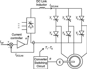
FIGURE 34.34 Schematic of a current-source inverter (CSI) driven synchronous motor.

The inverter drives the motor with quasi-squarewave current waveforms as indicated in Fig. 34.35. The current waveforms are switched according to the measured rotor position information, such that the current waveform in each phase has a fixed angular displacement, γ, with respect to the induced emf of the corresponding phase. Because of this, the drive is sometimes referred to as self-controlled. The angular displacement of these current waveforms (or their fundamental components) with the respective back-emf waveforms is indicated in Fig. 34.35. Because of the large dc-link inductor, the phase currents may be considered to remain essentially constant between the switching intervals. The quasi-square current waveforms contain many harmonics, and are responsible for large torque pulsations that may become troublesome at low speed.

FIGURE 34.35 Current waveforms in the delink current-source-driven motor.

In the forgoing scheme, the motor can be reversed easily by reversing the sequence of switching of the inverter. It can also be braked regeneratively by increasing the firing angle of the input rectifier beyond 90° while maintaining the dc-link current at the desired braking level until braking is no longer required. The rectifier now returns the energy of the overhauling load to the ac mains regeneratively.

In another scheme, which is preferred for lower capacity drives for which higher dynamic response is frequently sought, phase currents are regulated within the inverter. The inverter typically employs gate turn-off switches, such as the IGBT, and pulse-width modulation techniques, as indicated in Fig. 34.36. Motor currents are sensed and used to close independent current controllers for each phase. Normally, two current controllers suffice for a balanced star-connected motor. Three-phase sinusoidal ac currents are supplied to the motor, the amplitude and phase angle of which can be independently controlled as required. The references for the current controllers are obtained from a three-phase current reference generator that is addressed by the feedback of the rotor position. The rotor position is continuously measured by a high-resolution encoder. In this way, the current references, and hence the actual stator currents are synchronized to the rotor.

FIGURE 34.36 Control scheme of the SPWM current-source drive.

34.4.5 Brushless DC Operation of the CSI-driven Motor

The torque characteristic of the CSI drive scheme of the foregoing section can be easily analyzed using the phasor diagrams shown earlier, if the harmonics in the motor current waveform are neglected or if the motor current waveforms are indeed sinusoidal as in the second scheme described earlier. In the following analysis, it is assumed that the supply current waveforms are sinusoidal. It is also assumed that the phase angle of these current sources with respect to the induced voltage in each phase can be arbitrarily chosen.

The phase back-emf and the current waveforms and the phasor diagram of the nonsalient-pole motor are shown in Fig. 34.37. The phase angle γ between the E_f and I phasors and the RMS value (or amplitude) of I are determined according to the desired torque and power factor considerations. The developed torque is found from the phasor diagram to be

FIGURE 34.37 Phasor relationships of CSI-driven motor: (a) back-emf and current waveforms and (b) the phasor diagram.

(34.65)

If the angle γ = 0° is chosen, the familiar dc-motor-like torque characteristic is obtained. It should be noted from the forgoing that the developed torque at any speed is independent of R since a high-gain (stiff) current-source drive is used. Note also that the ratio E_f/ω at any operating speed is proportional to the amplitude of the stator flux linkage, λ_f, due to rotor excitation. For fixed rotor excitation this ratio is a constant.

Equation (34.65) indicates that the developed torque of a nonsalient-pole synchronous motor can be controlled by controlling the amplitude of the rotor field (field control), or more conveniently, by controlling the amplitude of the stator phase current. The highest torque per ampere characteristic is achieved when γ = 0°. Note that the operation with a fixed γ angle is key to this dc-motor-like torque characteristic.

34.4.5.1 Operation with Field Weakening

If the stator impedance drop is neglected, the maximum E_f is largely determined by the dc-link voltage and E_f = Kλ_fω implies that speed ω can be increased by decreasing λf. Consequently, the operation above base speed is normally achieved with field weakening. In this speed range, because of the limited dc-link voltage, the rotor field must be weakened; otherwise, the amplitude of the phase-induced emf will exceed the dc-link voltage and current control will not be effective. Field weakening is a means of keeping this voltage at the rated level for speeds higher than the base speed.

The flux linkage due to the rotor excitation, λ_f, can be adjusted when a variable rotor supply is available. This may also be achieved by demagnetizing the rotor mmf by using the mmf produced by the stator currents. For motors with permanent-magnet excitation, the latter is the only means of weakening the λ_f. Referring to the phasor diagram of Fig. 34.38, if I is made to lead E_f, the d-axis component of I, i.e. I_d, will lead E_f by 90°. The mmf due to I_d then opposes the rotor d-axis mmf. The net rotor flux linkage along the £j-axis is then given by

FIGURE 34.38 Field weakening using stator mmf.

(34.66)

where I_d is negative when I leads E_f. If the airgap is small, the d-axis component of the armature current may reduce the rotor flux to the required extent.

34.4.6 Operating Modes

A synchronous motor may be driven with a view to achieving various operating characteristics, such as power factor compensation, maximum torque per ampere characteristic, and field weakening. The power factor at which a synchronous motor operates is an important issue, especially for a large drive. A large angle θ between the input voltage and current phasors of the motor results in a poor overall power factor. Operation of the synchronous motor with a CSI which delivers the stator current waveforms with phase angle with respect to the respective phase back-emf waveforms that allows interesting power factor compensation possibilities. Consider the following three cases.

34.4.6.1 Case 1: Operation with I Lagging E_f

In this case, the motor is under-excited and I lags E_f, by an angle γ, as indicated in Fig. 34.39. The overall power factor in this case is lagging, since I lags V by an angle θ. The power-factor angle θ is larger than γ. Note that I_d now magnetizes the rotor field.

FIGURE 34.39 (a) Phase back-emf and current waveforms and (b) the phasor diagram with I lagging E_f.

34.4.6.2 Case 2: I is in phase with E_f, Maximum Torque per Ampere Operation (γ = 0°)

If γ = 0° is used, the motor input current i_a is in phase with the back-emf e_a, as indicated in the waveforms of Fig. 34.40a. From Eq. (34.65), the developed torque is given by

FIGURE 34.40 (a) Phase back-emf and current waveforms and (b) phasor diagram for I in phase with E_f.

(34.67)

Thus, for a fixed rotor excitation, the developed torque is the highest that can be achieved per ampere of stator current I. In other words, if γ = 0° is chosen, the drive operates with its maximum torque per ampere characteristic. From the phasor diagram of Fig. 34.40b, it is clear that the input current I phasor now lags the voltage V phasor at the motor terminals, (see the phasor diagram in the figure). Note that the level of E_f, which is determined by the level of excitation, also determines the angle θ to some extent. Clearly, when maximum torque per ampere characteristic is required, a power factor less than unity has to be accepted.

34.4.6.3 Case 3: Operation with I Leading E_f

If I is chosen to lead E_f, the overall power factor can be higher, including unity, as is indicated in Fig. 34.41. Note that the motor now operates with less than maximum torque per ampere characteristic. Note also that the d-axis component of I now tends to demagnetize the rotor and that the operation with field weakening is implied.

FIGURE 34.41 Back-emf and current waveforms and phasor diagram for I leading E_f.

With a CSI-driven motor, the amplitude and the angle of the phase current relative to the back-emf can be selected according to one of the desirable operating characteristics mentioned above. Additionally, other operational limits such as the inverter/motor current limit, the maximum stator voltage limit, and the maximum power limit can also be addressed. The amplitude of the stator current I clearly determines the developed torque of the motor. Consequently, the error of the speed controller is used to determine the amplitude of I. The overall control system with an inner torque loop can be described by Fig. 34.42.

FIGURE 34.42 Structure of a speed-control system with a CSI-driven synchronous motor.

34.4.7 Vector Controls

The foregoing controls were based on the steady-state equivalent circuit of the motor. Even though the torque Eq. (34.65) for a current-source drive evokes vector-control-like relationships, they do not address the dynamics of the current controls as is possible in an orthogonal reference frame. Using an orthogonal set of reference attached to the rotor, a simple set of decoupled, dc-motor-like torque control relationships is readily obtained. Following the transformation technique used in Section 34.3.4, the stator voltage equations of a synchronous motor with fixed rotor excitation in the rotor reference frame are

(34.68)

(34.69)

where all the quantities in lower case represent instantaneous quantities in the rotor dq-frame. The λ_f is the flux linkage per phase due to the rotor excitation, ω is the electrical angular velocity in rad/sec, and P is the number of pole pairs. Here, p is the time derivative operator d/dt. Assuming the magnetic linearity, the stator flux linkages are

(34.70)

Note that the Eq. (34.68) can be written down directly from Eq. (34.31), taking into account the fixed rotor excitation so that the third and fourth rows and columns of Eq. (34.31) may be dropped. Since the reference frame now rotates at the speed of the rotor, ω_e = ω. The induced back-emf due to the fixed rotor excitation occurs in the rotor q-axis and is included in Eq. (34.68), as a separate term. Similarly, the torque expression of Eq. (34.69) may also be written down from Eq. (34.41), using the flux linkages of Eq. (34.70).

Equations (34.67)–(34.69) are for a salient-pole motor for which L_d ≠ L_q. For a nonsalient-pole motor, L_d is equal to L_q and the developed torque is proportional to i_q only. In either case, the inner torque loop consist of two separate current loops; one for i_q and the other for i_q, as indicated in Fig. 34.43. The i_q current loop generally derives its reference signal from the output of the speed controller and constitutes the inner torque loop. The reference for the i_d current loop is normally specified by the extent of field weakening for which a negative i_d reference is used. Otherwise, the d–axis current is maintained at zero. Note that for large synchronous motors with variable external excitation, field weakening is normally applied through adjustment of the rotor excitation, using a spillover signal from the output of the speed controller.

FIGURE 34.43 Inner torque loop of a vector-controlled synchronous motor drive.

From Eq. (34.68), it is clear that the couplings of q- and d-axes voltages exist through the d- and q-axes currents, respectively, and the back-emf. During dynamic operation, such coupling effects become undesirable. The coupling effects of d- and q-axes currents and the back-emf into q- and d-axes voltages, respectively, can be removed by the feedforward terms shown in the shaded part of the block the diagram of Fig. 34.44 which also shows the two current-control loops. The two outputs v^*_d and v^* _q from the decoupled current controllers are transformed to the stator reference frame before being subjected to pulse-width modulators or hysteresis comparators. Note that the current references i^*_d, and i^*_q are obtained with due regard for the desired operating and limiting conditions as described in Section 34.4.5.

FIGURE 34.44 The d- and q-axis decoupling compensation.

Under this type of control, which is exercised in the rotor reference frame, the d- and q-axes currents are separately regulated. The purpose of the q-axis current controller is primarily to control the developed torque, especially for the nonsalient-pole motor. For this motor, the d-axis current is normally maintained at zero, when the motor is operated below the base speed. The d-axis current may be used to weaken the airgap flux so that the motor operates with a constant powerlike characteristic. It should be noted that the field weakening may also be carried out more directly by adjusting the rotor excitation current by using a spillover signal from the speed controller, when the base speed is exceeded.

The dynamic response of the drive under the vector control scheme indicated in Fig. 34.44 is the highest possible with a CSI drive. It should also be noted that the dq currents in the rotor reference frame vary only the mechanical dynamics of the rotor. In fact, they are dc quantities when the motor runs at a constant speed. Consequently, the following error (or lag) associated with tracking a sinusoidally time varying current reference, which is the case when current control is exercised in the stator a–b–c reference frame, can be reduced easily by using an integral-type current controllers.

34.5 Permanent-magnet AC Synchronous Motor Drives

34.5.1 Introduction

Since the introduction of samarium cobalt and neodymium–iron–boron magnetic materials in the 1970s and 1980s, synchronous motors with permanent-magnet excitation in the rotor have been displacing the dc motor in many high-performance applications. The trend is more noticeable in applications requiring high-performance motors of up to a few kilowatts. In low- to medium-power applications, the superior dynamics, smaller size, and higher efficiency of motors with PM excitation in the rotor, compared to all other motors, are well known. Prior to this development, the ferrite and alnico magnets were routinely used in small servomotors, with the magnetic excitation in the outer stator. Such motors need a brush-commutator assembly to supply power to the armature, that is a problem. Nevertheless, interesting low-inertia, low-armature inductance designs are possible that are desirable for servo applications. One such design is the pancake iron-less armature with the commutator-brush assembly directly located on the printed armature. These shortcomings of the commutator-brush are now avoided by locating the magnets in the rotor and by having three-phase windings in the stator that are supplied from an inverter.

The arrangement just mentioned is very similar to a conventional synchronous motor. This is particularly so when the stator windings and the rotor mmf are sinusoidally distributed.

Several rotor configurations of the PM synchronous motor have been developed, of which the important ones are indicated in Figs. 34.45–34.47.

FIGURE 34.45 Schematic of the cross section of a surface-magnet synchronous motor.

FIGURE 34.46 Schematic of the rotor cross section of an interior-magnet motor.

FIGURE 34.47 Schematic of the rotor cross section of a circumferential-magnet motor.

34.5.2 The Surface-magnet Synchronous Motor

The surface-magnet motor comes with the rotor magnets glued onto the surface of the rotor. An additional stainless steel (i.e. nonmagnetic) cylindrical shell may be used to cover the rotor in order to keep the magnets in place against centrifugal force in high-speed applications. Since the relative permeability of the magnetic material is very close to unity, the effective air-gap is uniform and large. The airgap is normally about 8 mm. Consequently, the synchronous inductances along the rotor d- and q-axes, as indicated in Fig. 34.45, are equal and small (i.e. L_d = L_q = L_s). The armature reaction in this type of motor is small.

The three-phase winding in the stator has sinusoidal distributed windings. In another form, the motor may have trapezoidal distributed winding, and the rotor mmf is also uniformly distributed. Such a motor, often called a brushless de (BLDC) motor because of its similarity to the inside-out conventional brushed PM DC motor, develops a trapezoidal back-emf waveform as indicated in Fig. 34.48, when it is driven at a constant speed. The back-emf waveforms have flat tops for nearly 120° in each half-cycle followed by 60° of transition from positive to negative polarity of voltage and vice versa. These motors are very suitable for variable-speed applications such as spindle drives in machine-tool and disk drives.

FIGURE 34.48 Back-emf of a trapezoidal waveform motor.

34.5.2.1 Control of the Trapezoidal-wave Motor

Neglecting higher-order harmonic terms, the back-emf in the motor phases may be as indicated in Fig. 34.49. Each back-emf has a constant amplitude (or flat top) for 120° (electrical) followed by 60° of transition in each half-cycle. The developed torque at any instant is given by

FIGURE 34.49 Back-emf and current waveforms and on-states of transistor switches in the trapezoidal-waveform motor.

(34.71)

It is readily seen that the ideal current waveform in each phase needs to be a quasi-square waveform of 120° of conduction angle in each half-cycle. The conduction of current in each phase winding coincides with the flat part of the back-emf waveforms, which guarantees that the developed torque, i.e. , is constant or ripple-free at all times. With such quasi-square current waveforms, a simple set of six opto-couplers or Hall-effect sensors would be required to drive the six inverter switches indicated in Fig. 34.36. The output current waveforms for the three-phase inverter and the switching devices that conduct during the six switching intervals per cycle are also indicated in Fig. 34.49. Since only six discrete outputs per electrical cycle are required from the rotor position sensors, the requirement of a high-resolution position sensor is dispensed with. Continuous current control for each phase of the motor, by hysteresis or PWM control, to regulate the amplitude of the motor current in each phase is normally employed. The operation of the BLDC motor drive is described in detail in Section 34.6.

Even though careful electromagnetic design is employed in order to have perfect trapezoidal back-emf waveforms as indicated in Fig. 34.49, the back-emf waveforms in a practical brushless dc motor exhibit some harmonics, as indicated in Fig. 34.48. If ripples in the back-emf waveforms are significant, then torque ripples will also exist when the motor is driven with quasi-square phase current waveforms. These ripples may become troublesome when the motor is operated at low speed, when the motor load inertia may not filter out the torque ripples adequately.

A second source of torque ripple in the permanent-magnet brushless de (PM BLDC) motor is from the commutation of current in the inverter. Since the actual phase currents cannot have the abrupt rise and fall times as indicated in Fig. 34.49, torque spikes, one for each switching, may exist.

Even though the PM BLDC motor does not have sinusoidal back-emf and inductance variations with rotor angle, the analysis of Section 34.4 in terms of the fundamental quantities will often suffice. The switching of the inverter using the six rotor-position sensors guarantees that the current waveform in each phase always remains in synchronism with the back-emf of the respective phase. Since the quasi-square phase current waveform in each phase coincides with the flat part of the back-emf waveform of the same phase, the angle γ is clearly zero for such operation. Thus, considering fundamental quantities, the motor back-emf and the torque characteristics can be expressed by

(34.72)

(34.73)

where K_E and K_T are equal in consistent units. Note that E and I are now RMS values of the fundamental components of these quantities.

34.5.2.2 Sensorless Operation of the PM BLDC Motor

In spindle and other variable-speed drive applications, where the lowest speed of operation is not less than a few hundred revs/min, it may be possible to obtain the switching signals for the inverter from the motor back-emf, thus dispensing with rotor-position sensors. The method consists of integrating the back-emf waveforms, which are the same as the applied phase voltage if the other voltage drops are neglected, and comparing the integrated outputs with a fixed reference. These comparator outputs determine the switching signals for inverter. It may be noted that the amplitude of the back-emf waveforms is proportional to the operating speed, so that the frequency of the comparator outputs increases automatically with speed. In other words, the angle γ and the current waveform relative to the back-emf waveform in each phase remains the same regardless of the operating speed. Integrated circuits are available from several suppliers, that perform this task of sensorless BLDC operation satisfactorily, covering a reasonable speed range.

34.5.3 The PM Sinewave Motor

The PM sinewave motor, which may also have magnets on the rotor surface or buried inside the rotor (as in the interior-magnet motor of Fig. 34.46), has sinusoidally distributed windings. The airgap flux distribution produced by the rotor magnets is also sinusoidal, arranged through magnet shaping. Consequently, the back-emf waveform of each phase is also a sinusoidal waveform, as indicated in Fig. 34.50, when the motor is driven at a constant speed.

FIGURE 34.50 Back-emf waveforms of a sinewave PM motor. Speed = 1815 rev/min.

It should be noted, however, that with magnets mounted on the rotor surface, the effective airgap is large and uniform so that L_d = L_q = L_s. Because of the large equivalent air-gap, these inductances are also small, and consequently, the armature reaction is small. As a result, this motor essentially operates with fixed excitation, and there is hardly any scope for altering the operating power factor or the rotor mmf, once the motor and its drive voltage and current ratings have been selected.

The PM sinewave interior-magnet motor, which comes with magnets buried inside the rotor as indicated in Figs. 34.46 and 34.47, has an easier magnetization path along the rotor q-axis, so that L_q < L_d. The small airgap implies that the inductances L_d and L_q may not be small, and hence may allow considerable scope for field weakening.

If the sinewave motor is supplied from an SPWM inverter, the analyses and vector diagrams of this motor are not different from those in Section 34.4 for the nonsalient-pole and salient-pole synchronous motor drives. The surface-magnet motor is more akin to the nonsalient-pole motor, since L_d = L_q = L_s, whereas the interior-magnet motor is more akin to the salient-pole motor because of the d- and q-axes inductances being unequal. Thus, the equations in Section 34.4 will apply equally well for this motor, both in the steady state and dynamically and for both voltage- and current-source supply.

34.5.3.1 Control of the PM Sinewave Motor

The sinusoidal back-emf waveforms imply that the three-phase motor must be supplied with a sinusoidal three-phase currents if a dc-motor-like (or vector-control-like) torque characteristic is desired, as was found in Section 34.4. For such operation, the phase currents must also be synchronized with the respective phase back-emf waveforms, in other words, with the rotor dq-reference frame. This implies the operation with a specified γ angle. Two implementations are possible.

In one scheme, the stator currents are regulated in the stator reference frame and the stator current references are produced with reference to the rotor position, as indicated in Fig. 34.51. The rotor position θ is continuously sensed and used to produce three sinusoidal current references of unit amplitude. The phase angle γ of the references relative to the respective back-emf waveforms is usually derived from the speed controller, which defines the field-weakening regime of the drive. The operating power factor of the drive may also be addressed using the γ angle control, as explained in Section 34.4.5. The amplitudes of these references are then multiplied by the error of the speed controller in order to produce the desired torque reference. In this way, both the RMS value I of the phase current and its angle γ with respect to E_f can be adjusted independently (which is equivalent to independent dq-axes current control). Three PWM current controllers are indicated, but two suffice for a balanced motor. Other types of current controllers, such as hysteresis controllers, may also be used.

FIGURE 34.51 Speed-controlled drive with the inner torque loop via current control in the stator reference frame.

In the second scheme, the motor currents are first transformed into the rotor dq-reference frame using continuous rotor position feedback and the measured rotor d- and q-axes currents are then regulated in the rotor reference frame, as indicated in Fig. 34.52. The main advantage of regulating the stator currents in the rotor reference frame, compared to the stator reference frame as in the first scheme, is that current references now vary more slowly and hence suffer from lower tracking error. At constant speed, the stator current references are in fact dc quantities as opposed to ac quantities, and hence the inevitable tracking errors of the former scheme are easily removed by an integral-type controller. The other advantage is that the current references may now include feedforward decoupling so as to remove the cross-coupling of the d- and q-axes variables as shown in the motor representation of Fig. 34.52. The latter scheme is currently preferred, since it allows more direct control of the currents in the rotor reference frame.

FIGURE 34.52 Block diagram of a current-controlled drive.

It should be noted that continuous transformations to and from rotor dq-axes are required; hence the rotor-position sensor is a mandatory requirement. Rotor-position sensors of 10–12 bit accuracy are normally required. This is generally viewed as a weakness for this type of drive.

The general torque relationship of a sinewave motor supplied from a current-source SPWM inverter is given by Eq. (34.69) which is rewritten here.

Precise control of the developed-torque control requires that both i_d and i_q be actively controlled in order to regulate it to the level determined by the error of the speed controller. For the surface-magnet synchronous motor, the large effective air-gap means that L_d ≈ L_q, so that i_d should be maintained at zero level. This implies that the i_d current reference in Fig. 34.52 should be kept zero. For the interior-magnet motor, L_q > L_d, so that i_d and i_q have to be controlled simultaneously to develop the desired torque. A few modes of operation are possible.

34.5.3.2 Operating Modes

34.5.3.2.1 Operation with Maximum Torque per Ampere (MTPA) Characteristic

In this mode of control, the developed torque T per ampere of stator current is the highest for a given rotor excitation. The combination of i_d and i_q that develops the maximum torque per ampere of stator current is indicated in Fig. 34.53. The reference signal for the inner torque loop normally determines the i_q reference; while the i_d reference is given by

FIGURE 34.53 i_d–i_q Trajectories for the maximum torque per ampere characteristic and for maximum voltage and current limits of an interior PM motor.

(34.75)

It should be noted that with i_d = 0, this mode of operation is achieved for the surface-magnet motor.

34.5.3.2.2 Operation with Voltage and Current Limits

The maximum current limit of the motor/inverter, I_smax, is normally imposed by setting appropriate limits on i_d and i_q such that

(34.76)

Equation (34.75) defines a circle around the origin of the i_d–i_q plane.

The available dc-link voltage to the inverter places an upper limit of the motor phase voltage, V_smax, given by

(34.77)

(34.78)

where the stator voltages v_d and v_q are expressed in the rotor reference frame, as in Eq. (34.68). Equation (34.78) is obtained from the voltage equation of Eq. (34.68) when the phase resistance R is neglected. Equation (34.78) defines elliptical trajectories that contract as speed increases. All the three modes of operation are included in Fig. 34.53.

34.5.3.2.3 Operation with Field Weakening

This mode of operation is normally required for operating the motor above the base speed. A constant-power characteristic is normally desired over the full field-weakening range. For a given rotor excitation of λ_f and developed power of P_O, the developed torque T and the net rotor flux linkage required for constant-power operation can be determined. From this, the limiting values for i_d and i_q, which further constrain the allowable i_d–i_q trajectory is also indicated in Fig. 34.53, can be determined.

The operating modes described in the preceding section are normally included in a trajectory controller that generates the references for i_d and i_q continuously, as indicated in Fig. 34.54.

FIGURE 34.54 i_d and i_q trajectory generation satisfying the desired operating modes.

34.6 Permanent-magnet Brushless DC Motor Drives

34.6.1 Machine Background

Anyone studying electric machines would be aware that the classical synchronous machine offers the possibility of the very highest efficiencies. These machines have the power-carrying conductors in the stationary part, therefore there is no need to transfer high power through a brush system. The field is provided on the rotating part either by an electromagnet, which does require some very low-power brushes or at best, by a permanent magnet with no power requirements at all.

This is clearly better than the traditional dc machine with high-power brushes and rotating conductors, with those conductors having a very poor path for heat to get away under overload conditions. You might ask, “why did we use so many of them?” It was of course because the dc machine offered the ability to control the speed fully and easily, which the synchronous machine, when running from the mains at a fixed frequency, was definitely not capable of. Thus, for example, all electric trains and trams built up to the 1980s, many of them still in service, use brushed dc motors.

The induction machine, the work horse of industry is quite efficient, but because of the need to carry magnetizing current in the stator as well as load current, and the existence of slip, it cannot be as good as the synchronous machine. It also innately has a very limited speed range.

All this changed with the advent of inexpensive, reliable power electronics. Quite suddenly power electronics engineers had the ability to vary both the frequency and the amplitude of an ac supply and thus to provide the holy grail of variable-speed ac motors. This was first applied to induction machines, with the simplest form of open-loop control. The complexity of control for synchronous machines added substantially to the cost and was not so appealing. Today the thought of putting a digital signal processor (DSP) or a microcontroller in a small motor controller is no longer as daunting as it was ten years ago, so the distinction between the complexity of a controller for induction machines and synchronous machines has almost disappeared.

Whilst power electronics radically changed our attitudes to electric machine design and operation, there was a second very important development which arrived on the scene at almost the same time; the appearance of very powerful rare earth permanent-magnet materials.

The first rare earth magnet material was Samarium Cobalt, used in very special applications such as space and defence, but it was then, and still is, very expensive. Neodymium–Iron–Boron (Nd–Fe–B) came next with even higher energy product. Energy product is a measure used to quantify the effectiveness of magnets. Nd–Fe–B began expensively, but has continued to drop in price at a spectacular rate and recently became cheaper than ferrites in term of dollars per unit of energy product.

Thus all the machines discussed here are permanent–magnet (PM) machines, in general using Nd–Fe–B magnets.

34.6.1.1 Clarifying Torque Versus Speed Control

As is well understood, given a fixed magnetic flux level, the magnitude of the current in a motor determines the magnitude of the torque out of the machine. In a general application if a torque is set, the speed is determined by the load. This is what happens when driving an automobile. The throttle or accelerator varies the torque. The speed can be very slow or very high for the same foot position, depending on the road conditions and vehicle motion history, even if the vehicle is in the same gear. This principle of torque control rather than speed control is fundamental to the operation of electric machines. When speed control is required in PMBDCMs, it is usual to implement torque control, with an extra outside control loop, like a cruise control in an automobile, to use the torque control to deliver speed control. So from here on the discussion will describe torque control for the variable-speed motor.

34.6.1.2 Permanent-magnet AC Machines

There are two quite different types of permanent-magnet ac machines, actually looking very similar in their physical realization but dramatically different in their electrical characteristics and in the way in which they are controlled.

34.6.1.2.1 Permanent-magnet Synchronous Machines

These are simple extensions of the classical synchronous machine, where all of the voltages and currents are designed to be sinusoidal functions of time, as they are in the synchronous machine when used as a supply generator. These machines are known as permanent-magnet synchronous machines (PMSMs) or brushless ac machines and are discussed elsewhere in this book. Whilst the application of sinusoidal waveforms everywhere is comforting to many and does result in less acoustic noise, less “stray losses” etc. there is in general a requirement to know the exact rotor angular position at every instant of time, with an accuracy in the order of one degree. This knowledge is then used to shape the current waveforms to be sure that they are in phase with the back-emf of the windings. Whilst much research is going on to run these machines without position sensors, the reality in the workplace today is that you need to include a relatively expensive shaft position encoder with your PMSM, if you wish to control it electronically.

34.6.1.2.2 Permanent-magnet Brushless DC Machines

A very much simpler possibility has emerged, which also gives the benefits of smooth torque and rapid controllability. This results in smaller minimum machine size, yielding maximum machine power density.

For this variant, the current waveforms and the back-emf waveforms are trapezoidal rather than sinusoidal. In this case, the machine is known as a permanent-magnet brush-less dc machine (PMBDCM), with waveforms as shown in Fig. 34.55.

FIGURE 34.55 Phase currents as functions of time and the flux density on the surface of the rotor as a function of angular position for a typical PMBDCM.

34.6.1.3 Brief Tutorial on Electric Machine Operation

The operation of electric machines can be explained in a variety of ways. Two possible and different methods are by:

(1) Using an understanding of the interaction of magnetic fields and the tendency of magnetic fields to align. This tendency to align is what provides the force that makes a compass needle swing around, until it aligns with the earth's magnetic field.

(2) Using the physical principle that “a current carrying conductor in a magnetic field has a force exerted on it.” This force is commonly known as the Lorentz force.

The difference between the two explanations is that the first method gives better “physical pictures.” However when one gets a little more serious, wanting to put in numbers, the force equations, whilst not greatly more difficult, are a little more challenging as they involve vector cross products.

With the second method, once the principle is accepted, there is a particularly simple scalar version of the force equation that very rapidly and simply gives numeric answers. The directions of the force, current, and motion are all orthogonal, i.e. at right angles and a formal exposition would again use a vector cross product. However, provided the rules learned in high school science are applied, the scalar version, F = BLI can be used, where F is the force in newtons, B is the flux density in Tesla, L is the length of the conductor in meters, and I is the current in amperes.

Let us try both the methods, on the simple machine of Fig. 34.56.

FIGURE 34.56 A simple motor with a single coil in the stator and a permanent-magnet rotor.

The rotor is a magnet with a north and a south pole, and there is a coil of wire in the slots in the stator. Current is shown going into the conductor called a at the top of the stator and coming out of the conductor called a' at the bottom. To simulate a real machine more closely, one should imagine putting a one turn “coil” of wire into the slot, with a connection made at the back of the machine to connect the top wire to the bottom, so that by applying a positive voltage to the top wire and a negative voltage to the end of the coil (the bottom wire), current will flow in at the top and out at the bottom as discussed previously.

Method 1

If the current is put into the top and comes out of the bottom as marked, then according to the right-hand rule (if you forget, then look at the Institution of Electrical and Electronic Engineers (IEEE) logo), magnetic flux will be forced to go through the center of the coil from right to the left, creating a north pole on the left. The flux will then double back through the iron frame of the motor to arrive back at the South pole on the right.

Figure 34.57 shows a computer generated magnetic field plot. This was produced using finite element analysis and modeling the stator as electrical steel, the volume in the center as air and injecting current into the coil.

FIGURE 34.57 A computer generated magnetic field for current in the windings and a stator made of electrical steel.

If the permanent-magnet rotor is then put inside the stator of Fig. 34.57, the rotor will align by rotating 90° counterclockwise.

Method 2

In this case, looking at Fig. 34.58, the conductor a will be immersed in a quite dense field produced by the magnets, with the flux lines going up the page in the rotor, across the airgap into the steel of the stator, heading down the stator to jump back across the lower airgap to return to the south pole. If a current is directed into the upper conductor and out of the bottom as before, it will produce force. Applying the direction rules associated with the Lorentz force, the force on the conductor will be to the right at the top and to the left at the bottom. Invoking Newton's third law, that action and reaction are equal and opposite, it is clear that if the wire is fixed, as it is, then there will be a force on the rotor to the left at the top and to the right at the bottom, thus the rotor will move counterclockwise as before.

FIGURE 34.58 Lorentz forces on conductor and rotor of a simple machine.

34.6.2 Electronic Commutation

If the rotor of Fig. 34.58 moves, then to keep it rotating in the same direction, sooner or later the current in the conductors must be reversed. The time at which that needs to be done is when the rotor has moved to an almost aligned position, so it is not really a matter of time, but a matter of rotor position. Since the rotor is a permanent magnet, it is a very simple matter to determine at least where the physical pole edges are, using simple, reliable and inexpensive Hall effect (HE) sensors. These are small semiconductor devices which respond to magnetic flux density. (There are many ways to sense the position of the rotor; however the remainder of this exposition will stay with the HE sensor for simplicity.)

A very simple motor, relying on the inertia of the rotor for continuous rotation, could have a control circuit which sensed when the rotor magnet was horizontal and then reversed the current in aa' of Fig. 34.58.

The traditional “H” bridge switching circuit shown in Fig. 34.59 does that very effectively. Switch drive logic must ensure that either S1 and S4 are on, or S2 and S3 are on and never S1 and S2 simultaneously, or S3 and S4 simultaneously. This simultaneous operation would provide a short circuit. When this happens due to errors in the switch drive signal it is called “shoot through.” There are generally important parts of the switch drive signal logic, discussed later, which try to make this impossible in normal operation.

FIGURE 34.59 An “H” bridge circuit that can reverse the current through aa', as drawn with mechanical switches.

In real motors, the permanent-magnet rotor field does not change instantaneously from north to south as the rotor rotates, so there would be reasonably large angles over which the torque could not be effectively produced. Also more coils are put in so that the space of the machine frame is used more efficiently.

The use of three “phases,” as in Fig. 34.60, is very common. There are many things which balance naturally in a three-phase system and it is the simplest system with which it is possible to develop constant and unidirectional torque at all times and positions.

FIGURE 34.60 The physical layout of a three-phase PMBDCM.

A very common method has developed, known as “six step switching.” In this system, three phases are used. They are connected in star and there is a space between each of the magnet poles on the rotor and the two phases are activated at any one time, the third “resting” as the space between the magnet poles passes over it.

While the motor in Fig. 34.60 looks just like a three-phase synchronous machine, its operation is rather different.

As stated above, the windings are invariably star connected, as shown in Fig. 34.61.

FIGURE 34.61 The schematic connection of the windings shown in Fig. 34.60.

Six Step Switching Explained

Consider the coil aa', as shown in Fig. 34.60 and also diagram-matically in Fig. 34.61. Current driven into the a terminal, coming out of the a' terminal, will produce, as discussed before, flux from left to right, as shown here.

Obviously if the current direction in aa' is reversed, the flux will be

Similarly if current is driven into b and out of b' flux will result

And if it is reversed,

Finally, if current is driven into c and out of c', flux will result

And if it is reversed,

The permanent-magnet rotor would tend to align with the flux arrow shown in each of the states above, as discussed under machine operation, Method 1.

Now if the motor is wired in star as shown in Fig. 34.61, and a steady current is driven into a and out of b, the first and the fourth cases above occur at the same time. They add to produce a resultant,

and the rotor will tend to align with this resultant.

The Hall effect sensors are positioned so that just as the rotor gets to within 60° of being aligned, another arrangement of the windings is energized, and the field jumps forward another 60°, so the rotor is 120° away from being aligned. The rotor is always an average of 90° away from its desired position!

If a controller has input power from positive and negative of a dc supply and outputs to the terminals a, b, and c only, then the sequence of connections shown in Table 34.2 will produce the resultant flux directions as shown, providing continuous rotation.

TABLE 34.2 The sequence of connections which results in counterclockwise continuous rotation of the rotor of the PMBDCM of Fig. 34.60

The switching of Table 34.2 is simply achieved by a variant of the “H” bridge, as shown in Fig. 34.62. This process of switching current into different windings is called commutation and is the equivalent of the sliding brush contacts in a traditional brushed dc machine.

FIGURE 34.62 The switching circuit used for commutation of a PMBDCM.

34.6.3 Current/Torque Control

You may have noted that the discussion has been about current in the windings rather than the voltage across them. In very simple small brushless DC machines, like the one in the muffin fan in your computer power supply, voltages are connected directly to the windings. For these small motors, the resistance of the windings is relatively high and this helps limit the actual current that flows and swamps inductive effects.

There is an extra difficulty that must be addressed with high-performance, high-efficiency, well-made machines, and it adds another layer to the control of the motor. Such machines can easily be designed with very low resistance windings. It is not uncommon to have windings for a 200 V machine at the 20 kw level with the winding resistances less than 0.1 Ω.

When starting, or at a low speed, the current in a winding is limited only by the very low resistance and, for the machine above by Ohm's law, I = E/R would result in more than 2000 amperes.

The most common requirement for a steady current in the windings is to provide a steady torque. There is always a back-emf generated in the windings whenever the motor is rotating, which is proportional to speed and subtracts from the applied voltage. Thus currents cannot be determined just by terminal voltage. The winding does however have inductance. Whenever the copper conductors are put in coils in an iron structure, particularly if there are low reluctance magnetic paths with only small airgaps, the creation of quite large inductances cannot be avoided. These are used to very good effect.

The nature of inductance is that when a voltage is applied to an inductor, instantaneous current does not result, rather the current begins to increase and ramps up in a quite controlled fashion. If the voltage across the inductor is reversed the current does not immediately reverse, rather it ramps down, will go through zero and reverses if the reversed voltage is left there long enough. However, if the voltage is alternated by switching rapidly, as can be done with power electronics, the current can be controlled to ramp-up and ramp-down either side of a desired current, staying within any determined tolerance of that desired current.

Figure 34.63 looks very much like the simple “H” bridge commutation circuit, but is performing a very different function. It is controlling the current amplitude to stay within a desired band. If S1 and S4 are turned on then the current will begin to increase from left to right in the winding. The current sensor in the circuit detects when the current reaches a value of half the hysteresis band of the comparator above the desired current level and initiates turn-off of S1 and S4 and turn-on of S2 and S3. (If they were all turned off at once, the inductive nature of the circuit would produce very high voltages which would cause arcing in mechanical switches, or breakdown and failure of semiconductor switches, see later.) The current then begins to reduce. It reduces a small amount, down to half the hysteresis band of the comparator below the desired current level and then the switches reverse again. Thus a desired current level is achieved, with an arbitrarily small triangular ripple superimposed, as shown in Fig. 34.64.

FIGURE 34.63 Hysteresis band current control using pulse-width modulation (PWM).

FIGURE 34.64 Hysteresis band current control and PWM waveforms.

The general process of controlling by switching a voltage fully on or fully off at high speed is called pulse width modulation (PWM) and the specific method of current control achieved above with PWM, is called hysteresis band current control (HBCC).

Of course to keep this current ripple small, the switching may need to be very fast, but with the modern semiconductor switches there is no great problem up to 100 kHz for small machines and typically above 15 kHz for acoustic noise reasons, for machines rated up to several hundred kilowatts.

A perceived “drawback” of HBCC is that the switching frequency is determined by the circuit inductance, the width of hysteresis band, the back-emf, and the applied voltage, ranging very widely in normal operation. It is not difficult, but it is a little more complicated, to use a fixed frequency, and a linear analog of the current error to modify the pulse width of the PWM signal.

34.6.3.1 Switching Losses

There is a practical limit to how often semiconductor switches can be operated. At every change of state, if the switch is carrying current as it is opened, then as the voltage rises across the switch and the current through it falls, there is a short pulse of power dissipated in the switch. Similarly, as the switch is closed, the voltage will take some time to fall and the current will take some time to rise, again producing a pulse of power dissipation. This loss is called switching loss. Fairly obviously it will represent a power loss proportional to the switching frequency and so the switching frequency is generally set as low as it can be without impinging on the effective operation of the circuit. “Effective operation” might well include criteria for acoustic noise and levels of vibration.

34.6.3.2 High Efficiency Method of Managing the Switching in the H Bridge

A very common way to control the current with the smallest number of switching transitions is to combine HBCC with, for example, alternating only S1 and S2 in Fig. 34.65 leaving S4 on all the time, on the understanding that there will be a back-emf in the winding and the current can still be increased or decreased as desired.

FIGURE 34.65 H-bridge switching with one switch steadily on and a back-emf.

Thus when the motor is rotating and the back-emf is somewhere between zero and the rail voltage, alternating two switches rather than four will still allow current control in the coil, using for example HBCC, exactly as before.

This is a very common control scheme and will need some extra logic to reverse the direction of rotation of the motor, by either turning S4 off and S3 on continuously, or by swapping the control signals to the left and right “legs.” For full-servo operation normal H-bridge switching can be used and the logic is slightly different, but not significantly more complicated. However, following the discussion above, the switching losses will be higher.

34.6.3.3 Combining Commutation and PWM Current Control

The real break-through is that one set of six switches can be used for both PWM and commutation. That is the clever part and also the confusing part when one first tries to understand what is going on.

Thus, in a controller there are two control loops. The first is an inner current loop switching at, for example, 15 kHz to control carefully and exactly the current in two of the coils. Then at a much lower rate, for example at 50 times per second at 3000 rpm, the two coils doing the work are changed according to Table 34.2, controlled by an outer commutation loop, using information from the Hall effect shaft position sensors.

A complete controller is shown in the block diagram form in Fig. 34.66. Various aspects of this block diagram will now be examined and explained in detail.

FIGURE 34.66 A complete controller showing the two feedback paths, one for the position sensors and one for the current sensors.

34.6.3.3.1 Hardware Details–Semiconductor Switches

The three most likely semiconductor switches for a six step controller are the bipolar junction transistor (BJT), the metal-oxide silicon field effect transistor (MOSFET) and the insulated gate bipolar transistor (IGBT). Older controllers used BJTs, however contemporary controllers tend to use MOSFETs for lower voltages and powers and IGBTs for higher voltages and powers. Both of these devices are controlled by a gate signal and will turn-on when the voltage of the gate above the source or emitter is greater than a threshold, which is typically about 5 V. Use of about 10 V is common. The devices are thus off when the gate voltage below the threshold. Systems typically use zero volts for the off state. The controller of Fig. 34.66 shows MOSFETs used for the six switches.

The trick is that the voltage at terminal a, also S1's source, is either ground or the positive potential of the battery, depending on which switches are on. Driving S2, S4, and S6 is easy since the MOSFET sources are all at the potential of the negative rail and the lower gate drive signals are referred to this rail.

There is a range of dedicated integrated circuits which can drive the switches S1, S3, and S5, and which use a “charge pump” principle to generate the drive signal and the drive power internally, all related to the MOSFET source potential. Various approaches to this technical challenge of providing a floating gate drive are commonly discussed under the generic heading of “high side drives.”

For the most sophisticated drives, transformer coupling is used to provide a tiny power supply especially for the isolated gate drive and send the control signals either through an opto-coupler or a separate transformer coupling. The high-side drive problems here are exactly the same as those encountered in the traditional buck converter, or in drives for induction motors and PMSMs.

34.6.3.3.2 Dead Time and Flyback Diodes

Two issues have been mentioned above that must be addressed when using high-speed electronic switches in inductive circuits.

The first, in Section 34.6.2 “Electronic Commutation” was that care should be taken to ensure that the upper and lower switches in the same “leg,” (e.g. S1 and S2) are never turned on at the same time. If the controller attempts to turn one off and the other on at the same instant and switch turn-off is slower than turn-on (as it is with BJTs and IGBTs), then a short circuit will result for a brief time. The bus capacitor is usually very large to provide ripple current (see later) and usually of very high quality being fabricated especially for power-electronic applications, and can easily provide thousands of amperes for a few microseconds, which is enough to destroy the semiconductor switches.

The second issue, discussed in Section 34.6.3 “Current/Torque control” is that one cannot turn-off both switches in a leg at the same time, even for a few nanoseconds, since the voltages resulting from attempting to interrupt current in an inductor will cause avalanche breakdown and failure of the semiconductors. This sounds like quite a dilemma.

There is actually a very simple and effective solution. At any transition, the control circuitry ensures that the active switches are all turned off before any switch is turned on, usually for a few microseconds. This is known as “dead time” and its provision is an essential part of most of the dedicated integrated circuits in use. Then a “flyback”/“freewheel” diode is put in anti-parallel with each semiconductor switch and this provides the current path during dead time. These diodes are shown in Fig. 34.66.

The diode has a little more loss than the switch, since the diode forward drop is more than the switch drop. This is significant in a low voltage controller. However, as stated above, for a low voltage controller, MOSFETs are the device of choice. They have a lesser known property, that when gated on, they can carry current in both directions. Intriguingly the “on” state resistance is lower in reverse than in the forward direction! Thus for low voltage controllers, when the switch forward drop represents a significant contribution to losses, the MOSFET is turned on after dead time for both the current directions. Thus the higher loss in the diode is only for a few microseconds.

It is not difficult to produce from the PWM signal an “I up” logic signal which is used to cause the current to increase and an “I down” logic signal used to decrease it, with the timing as shown in Fig. 34.67. The function can be executed in sequential logic, or with the simple analog timing circuits.

FIGURE 34.67 Dead time introduced into the PWM logic signal, for switch drive.

A. Semiconductor Detail

In MOSFETs and most IGBTs, there is a diode already within the device; it is unavoidable and results from the fabrication processes. In modern power semiconductors, this intrinsic diode is optimized to be a good switching diode. The serious designer, however, will check the specifications for reverse recovery of this diode, since in highly optimized controller designs, reverse recovery losses in the intrinsic diode can be significant and are very difficult to control. In low voltage controllers, you can put a Schottky diode in parallel with the intrinsic body diode. The Schottky diode, with its lower forward voltage drop will tend to take the current and has no reverse recovery problems, but the current must commutate to it from the semiconductor die and the inductance of the connections is critical.

B. The Smoothing Capacitor on the Input to the Controller

This is a substantial capacitor, often very expensive, (it is shown in Fig. 34.66 as C in) and its design is quite challenging. The issue of smoothing is quite serious. If there are high-frequency or sudden current changes in the leads from the dc supply to the controller, they will radiate electromagnetic energy. Good design will limit the length of conductors in which the current is changing rapidly. Thus, a very large capacitor is placed physically as close to the positive bus of the switches as possible, aiming to have a steady current in the longer conductors from the dc supply, up to the capacitor. When the motor is running at, say, half speed and providing large torques, a very high level of ripple current is carried by this capacitor. Kirch-hoff's current law (KCL) must be applied at node A, as shown in Fig. 34.68. Good capacitors have a ripple current maximum buried away in their specification sheet. It turns out that in general, the size of the capacitor in a given design has very little to do with how much voltage ripple you can tolerate at the bus, but rather is determined by the ability to carry the ripple current without the capacitor heating up and failing. It has been known that the small electrolytics in prototype controllers mysteriously explode. On searching, it is found that they are in parallel with the main capacitor and quite close to it, so they carry a lot of ripple current, then heat up and explode!

FIGURE 34.68 Kirchhoff's current law at node A.

34.6.4 The Signal Processing for Producing Switch Drive Signals from Hall Effect Sensors and Current Sensors

34.6.4.1 Operation of the Hall Sensors

The flux density directly under a magnet pole can be anywhere from 500 to 800 millitesla with Nd–Fe–B magnets. Hall effect (HE) sensors with a digital output, called Hall effect switches, change state at very close to zero flux density. Thus, they will change state when the north and south pole are equidistant from them, so that for example, in Fig. 34.69, the switch HE1 is just changing state with the rotor as shown.

FIGURE 34.69 Possible Hall effect switch positions in a three-phase machine.

In practice, a motor designer needs to consider what magnetomotive force comes from the current in the windings which might result in flux which would trip the HE sensor at a slightly different time. If you follow all the above logic about six step switching, you will see that you only need the magnet poles to have a span of a bit more than 120°. Using 180° magnet poles can add considerably to the cost, as well as having an impact on such things as cogging torque. Actual designs often add extra “sense” magnets to cover 180° just at the circumferential strip where the HE switches are located, adding minimally to the magnet mass and ensuring good and accurate triggering.

However, if the switches operate as above, then Table 34.3 will result for the HE switches located as shown in Fig. 34.69.

TABLE 34.3 Hall effect switch outputs for rotor positions as shown, HE switches placed as in Fig. 34.69

34.6.4.2 Sensing the Current in the Motor Windings

Figure 34.66 shows two current sensors. In the most sophisticated systems, there are two current sensors, one in each of the two motor phases. The current sensing is done at the winding and isolated with either an HE sensor in a soft ferromagnetic magnetic core surrounding the conductor (commercial items are available), or by using a resistive shunt sensor and some accurate analog signal isolation/coupling through transformers or opto-couplers. The isolation is necessary since the potential at points a, b, and c is either the dc bus voltage or zero, depending on which switches are on, so that any current measure such as the small voltage across a shunt is superimposed on these very large voltage changes. This is a very similar problem to that for the high side gate drives discussed earlier. The current in the third winding is determined by the algebraic application of KCL, given the other two readings.

Simple controllers sometimes avoid the complexities of isolated current measurement and instead measure the current in the return negative supply, for example from the bottom of the three lower switches to the bottom of the supply smoothing capacitor. This arrangement senses current when an upper and a lower switch is on, but not when the current is being carried in flyback diodes or by two lower switches. While it is inexpensive, it does not provide fully accurate control. The system works because the current should be decreasing when a measure is not available, heading towards zero, so switch or system failure due to over-current should not occur.

34.6.4.3 Management of Current Sensing

The controller must select the right current to increase or decrease, dependent on rotor position. The following convention is adopted. Positive current provides torque in the counterclockwise direction and therefore goes into winding a, b, or c.

All systems are capable of regeneration, which implies that negative torque can be commanded (without reversing the direction of rotation) to make the machine operate as a generator, developing retarding torque.

Thus for the above sequence of sector determinations, referring back to Table 34.2, the output of current sensors should be directed to the current controller as shown in Table 34.4.

TABLE 34.4 Current sensors to use as input to the current controller, for each of the six rotor position sectors

Hall effect switch outputs (HE1, HE2, HE3)	Monitor current as read by
100	Negative of (sensor a+ sensor b)
110	Negative of (sensor a+ sensor b)
111	Sensor b
011	Sensor b
001	Sensor a
000	Sensor a

The addition and negation required can be carried out with the standard operational-amplifier circuitry. The three required analog measures are then fed to a three to one analog multiplexer, gated from the HE switch signals suitably processed in combinational logic. The resulting single analog output is fed to the current comparator.

34.6.4.4 Distribution of Control Signals to the Switches

Given that the dead time is introduced elsewhere in sequential logic, or with timing circuits, it is a simple matter to develop the combinational logic for directing, or steering, the switching signals to the right switches. A typical scheme for a specific controller is shown in Table 34.5.

TABLE 34.5 Distribution of control signals to the switches using “High Efficiency Method of Managing the Switching in the H Bridge”

It is usual also to include some shutdown logic from dedicated protection circuits, for example sensing over-current, over-bus voltage, under voltage for gate drive and over-temperature both in the motor and in the controller power stage. For simplicity, this is not shown in the table.

..................Content has been hidden....................

You can't read the all page of ebook, please click here login for view all page.

Table of Contents for 34. Motor Drives

Create new playlist

Sign In

Sign Up

34

Motor Drives

34.1 Introduction