
43
Computer Simulation of Power Electronics and Motor Drives
Center for Pulsed Power and Power Electronics, Department of Electrical and Computer Engineering, Texas Tech University, Lubbock, Texas, USA
43.1 Introduction
43.2 Use of Simulation Tools for Design and Analysis
43.3 Simulation of Power Electronics Circuits with PSpice®
43.4 Simulations of Power Electronic Circuits and Electric Machines
43.5 Simulations of AC Induction Machines Using Field Oriented (Vector) Control
43.6 Simulation of Sensorless Vector Control Using PSpice®
43.7 Simulations Using Simplorer®
43.8 Conclusions
43.1 Introduction
This chapter shows how power electronics circuits, electric motors, and drives, can be simulated with modern simulation programs. The main focus will be on PSpice®, which is one of the most widely used general-purpose simulation programs and Simplorer®, which is more specialized towards the power electronics and motor drives application area. Ali Ricardo Buendia, who obtained his M.S.E.E. degree from Texas Tech University, has created the examples for Simplorer®. The PSpice® examples have been developed for the free student version of OrCAD Capture 9.1 from Cadence. The author found the use of examples that can be run on the student version very beneficial in an educational environment, since such examples can be shared with students to enhance their understanding of the lecture material. This shall by no means lead to the conclusion, that the programs and simulations presented here cannot be used for serious professional work. In fact, the author has used these tools with great success in many research and consulting projects. In addition to the programs mentioned above, MathCAD® has been used to derive and present the underlying equations. The advantage of using MathCAD® for this purpose is that in MathCAD® it is possible to check equations by actually executing them.
The examples have been developed to illustrate advanced techniques for simulation of systems from the power electronics and drives area but not to teach the basic features of the individual programs. It is assumed, that the reader will familiarize themself with the basics on how to run the programs using the accompanying documentation. In addition, it is assumed, that the reader is familiar with the basics of power electronics and electric machines, specifically AC induction machines. For a review the reader shall be referred to [1] for power electronics and [2, 3] for induction machines.
43.2 Use of Simulation Tools for Design and Analysis
It is appropriate to reflect upon the value of simulations and its place in the design and analysis process before any in-depth discussion of specific simulation examples. Computer simulations enable engineers to study the behavior of complex and powerful systems without actually building or operating them. Simulations therefore have a place in the analysis of existing equipment as well as the design of new systems. In addition, computer simulations enable engineers to safely study abnormal operating or fault conditions without actually creating such conditions in the real environment.
However, the reader should be reminded that even the most modern simulation programs cannot perfectly represent all parameters and aspects of real equipment. The accuracy of the simulation results depends on the accuracy of the component models and the proper identification and inclusion of parasitic circuit elements such as parasitic inductance, capacitance, and mutual coupling. Accuracy of component models in this context shall not mean that the model is actually faulty but rather that the limitations of the model are exceeded. For example, if the transformer inrush phenomenon were to be studied using a linear model for a transformer, the simulation would not yield useful results.
In particular, the precise prediction of voltage and current traces during fast switching transitions in power electronics circuits has been proven to be difficult. To obtain useful results, extensive experimental validation, advanced device models (and the values for their parameters!), and detailed knowledge of parasitic elements, including the ones of the packaging of the circuit elements, are necessary. In addition, numerical convergence is often a problem, if gate-drive signals, with rise and fall times as steep as in real circuits, are applied. Therefore, the exact prediction of waveforms during switching transitions shall be excluded from the discussions in this chapter. Consequently, the author prefers to measure parameters such as voltage rise and fall times, over and undershoot etc. on actual circuitry in the laboratory.
Sometimes, users of PSpice® claim that the convergence problems are so severe, that it's use for simulations of power electronics circuits is just not possible or worth the effort. However, this is absolutely not true and with the proper techniques of gate signal generation, we can simulate just about any given circuit with little or no convergence problems. In addition, if convergence problems are avoided, simulations run much faster and larger numbers of individual transitions can be studied. This is achieved by generating gate signals that are slightly less steep than in real circuits using analog behavioral elements. This gives a lot of insight into the cycle-by-cycle as well as the system level behavior of a power electronics circuit. In this fashion, the function of an existing, as well as the expected performance of a new proposed circuit can be studied. An excellent application for these cycle-by-cycle simulations is the development and verification of control strategies for the power semiconductors.
Analog behavioral modeling (ABM) techniques included in PSpice® can be used to study large and complex systems like the control of induction machines using field oriented (also called vector) control techniques. Examples are given that replace the power electronics inverter with an ABM source that produces voltages, which represent the short-term average (filtering away the voltage components of the switching frequency and above) of the output of a three-phase inverter. These examples represent pure system level simulations, which could have also been done using programs like MatLab/Simulink®. However, circuit simulation programs provide the option of studying actual circuit level details in complex systems. To demonstrate this capability, the start-up of an induction motor, fed by a three-phase metal oxide semiconductor field effect transistor (MOSFET) inverter, is presented.
In all modeling cases, the user needs to define the goal of the simulation effort. In other words, the user must answer the question “What information shall be obtained through the simulation of the circuit or system?” The user must then select the appropriate simulation software and the appropriate models. This process requires a detailed understanding of the properties and limitations of the device models and the sensitivity of the results to the model limitations. In order to obtain such an understanding, it is often recommended and necessary to perform numerous simulation test runs, carefully scrutinize the results and compare them with measured data, results from other simulation packages or otherwise known facts.
43.3 Simulation of Power Electronics Circuits with PSpice®
The first example of a power electronics circuit is a step-down (also called buck) converter with synchronous rectification. For the purpose of synchronous rectification, the diode, which connects the inductor to ground in the regular circuit, is replaced with a power MOSFET transistor. The benefit of this circuit is that the power MOSFET represents a purely resistive channel in the on state. This channel does not have a residual, current independent, voltage drop like the p-n junction of a diode. Therefore, the voltage drop across the MOSFET can be made lower than what can be achieved with diodes. The results are reduced losses and increased efficiency. To achieve this, the lower MOSFET must be turned on whenever the upper MOSFET is turned off and the current in the inductor is positive. If the current in the inductor is continuous, the drive signal for the lower MOSFET is simply the inverted drive signal for the upper MOSFET. However, if the current in the inductor is discontinuous, the drive signal for the lower MOSFET must be cut off as soon as the current in the inductor goes to zero.
Figure 43.1 shows a simulation setup for a synchronous buck converter that can operate correctly for continuous as well as discontinuous inductor current. As mentioned before, the key element of this example is the circuit for the generation of the gate-drive signals for the MOSFETs. For clarity, this circuit has been realized using only standard elements from the libraries of the evaluation version. The basic principle of the operation of the gate-drive circuit is the well-known carrier based scheme, where a control voltage is compared with a triangular carrier with fixed amplitude. An “ABM” block, shown in the lower left part of Fig. 43.1, generates the triangular carrier. Equation (43.1) shown below gives the closed form equation for the triangular carrier wave. The output range of the function shown in Eq. (43.1) is between 0.0 and 1.0.
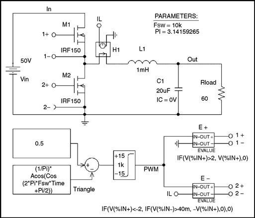
FIGURE 43.1 Simulation setup for a synchronous buck converter.
![]() (43.1)
(43.1)
For the generation of the gate-drive signals, the carrier wave is compared with a control signal that can have values between 0.0 and 1.0, corresponding to a duty cycle input between 0 and 100%. Feeding the difference of the carrier wave and the control signal into a soft comparator generates the primary PWM signal. Careful inspection of the implementation of the soft-limiter element provided in the evaluation version of PSpice® shows that it uses a scaled hyperbolic tangent function. Figure 43.2 shows a plot of a hyperbolic tangent function. It can easily be seen, that the result of the soft-limiter is an output signal with smooth transitions, which is crucial to avoid convergence problems in PSpice®. The soft-limiter used here has an upper and lower limit of ± 15 V and a gain (steepness control for the tanh function) of 50.
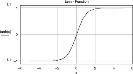
FIGURE 43.2 Plot of a hyperbolic tangent function used to generate smooth PWM signals.
Figure 43.3 shows the output of the simulation run for the synchronous buck converter. The top-level graph shows the generated triangle carrier. It has a frequency (Fsw, see parameter statement in Fig. 43.1) of 10 kHz. This frequency has been chosen rather low to improve the readability of Fig. 43.3. In the graph of the triangle voltage in Fig. 43.3, the gate-drive signals are shown for both MOSFET transistors. Please note, that the gate-drive signal for the lower MOSFET is vertically shifted by 30 V in order to separate the traces for readability. The graph below the gate-drive signals shows the inductor current. It can be seen that the current is discontinuous after the initial inrush peak. The inrush peak is caused by the fact that the capacitor is initially discharged (IC = 0 V). It is evident, that the gate-drive signal of the lower (synchronous rectification) MOSFET is appropriate for the inductor current. The bottom trace shows the capacitor voltage, which has a steady-state value of slightly more than 0.5 × 40 V (0.5 = 50% being the duty cycle and 40 V being the input voltage) due to the fact that the inductor current is slightly discontinuous even at steady-state conditions. To test the gate-drive circuit for the lower MOSFET, the load has been chosen such that the steady-state current would be discontinuous. Following the soft-limiter are two voltage-controlled voltage sources that generate isolated gate-source voltages of 15 V for the on condition and 0 V for the off condition of the MOSFETs. To enable operation with discontinuous inductor current, the source “E—” in Fig. 43.1 also monitors the polarity of the inductor current through a current-controlled voltage source “H1” with unity gain.
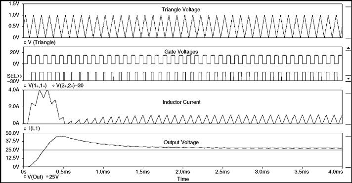
FIGURE 43.3 Output waveforms for the synchronous buck converter.
In addition to the cycle-by-cycle simulation of a DC-DC converter, it is also possible to use a time-averaged replacement for the MOSFET transistors used in the circuit in Fig. 43.1. In fact, a common time-averaged model can be used for the buck, the boost, the buck-boost, and the Cuk converter as long as they operate with continuous inductor current. The time-averaged model has the advantage that it can run much faster since it does not have to follow each switching transition. It is also possible to perform DC and AC sweep analyses. A DC sweep would sweep the duty cycle over a wide range and show the output voltage as a function of the duty cycle. An AC sweep analysis would sweep the frequency of an AC signal, which is superimposed on top of the duty cycle bias signal. The AC sweep allows the study of the behavior of the converter, including a feedback control system, in the frequency domain for traditional stability analysis and system tuning. A detailed description of this time-averaged modeling technique, including detailed examples is given in [4].
To illustrate the capabilities of the PSpice® simulation program, the next example shows a complete three-phase inverter bridge using six power MOSFETs. This circuit is shown in Fig. 43.4. Note that free-wheeling diodes are an integral part of every power MOSFET and are not shown separately. The inverter drives a three-phase load, which could represent an induction motor for a singular operating point. The load is connected to the inverter output terminals with so-called connection bubbles. Due to the number of elements involved, the circuit for the gate drive-signal generation is contained in a hierarchical block. Blocks like this are available from the main toolbar in the schematic editor. Selecting “Descend Hierarchy” for the block called “PWM_Generator” reveals the subcircuit which is shown in Fig. 43.5.
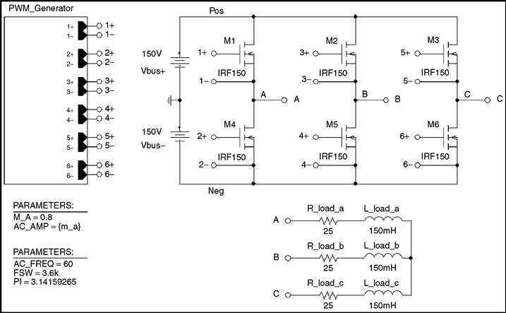
FIGURE 43.4 Circuit for a three-phase inverter with MOSFETs.
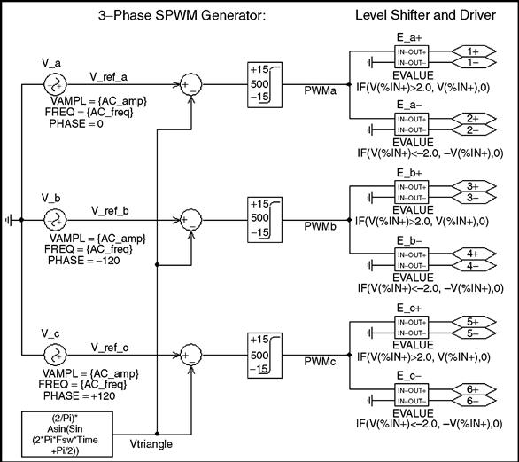
FIGURE 43.5 PWM generation subcircuit for a three-phase MOSFET inverter.
The hexagonal shaped symbols named “ 1+,” “ 1−,” “ 2+,” etc. are called interface ports. These interface ports provide the connection between the subcircuit and the ports of the hierarchical block above. Here the connection is to the ports (dots) on the “PWM_Generator” block. The interface ports are created by simply drawing a wire up to the boundary of the block. The name of the port is initially generic, “Px,” where x is a running number, but can be easily edited by double-clicking on the generic name. After drawing a block and creating all the ports, right-clicking the “Descend Hierarchy” will open up a schematic page for the subcircuit which has all the appropriately named interface ports already in it. Additional details on hierarchical techniques can be found in [5].
The circuit shown in Fig. 43.5 is similar to the gate-drive generation circuit discussed before. Circuits like the circuit shown in Fig. 43.1, compare a triangular carrier with one or more reference signals. In this case, three reference signals, one for each phase, are used. The triangular carrier signal is symmetrical with respect to the time axis. The values cover the range from — 1.0 to 1.0. The equation for the triangular carrier for PWM modulation for AC reference signals is given by the Eq. (43.2).
![]() (43.2)
(43.2)
The three reference signals are sinusoidal signals with equal amplitude and a relative phase shift of 120°. For linear modulation, the amplitude range of the reference signals is limited to the amplitude of the triangular carrier, e.g. 1V. The ratio of the reference wave amplitude and the (fixed) carrier amplitude is called amplitude modulation ratio “m_a” In the circuit shown in Fig. 43.4 “m_a” has a value of 0.8. This value is defined by a parameter symbol and represents a global parameter, which is visible throughout all levels of the hierarchy. The phase to neutral voltage amplitude of each inverter leg is equal to “Vbus+” (shown in Fig. 43.4) multiplied with the amplitude modulation ratio. The frequency and waveshape of the phase to neutral voltage of each phase leg is equal to the reference waveform, if the high-frequency components resulting from the carrier wave are filtered away. This way, each inverter leg can be viewed as a linear power amplifier for its reference voltage. In fact, in drive applications, inverters are often called “servo-amplifiers.” The load typically reacts only to the low-frequency components of the inverter output voltage. The high-frequency components, which include the triangular carrier frequency (also called switching frequency) and its harmonics, are typically “just a blur” for the load. This is especially true in recent times, where switching frequencies of 20 kHz and above are possible. As an added benefit, audible noise is avoided at these frequency levels.
The circuit involving the soft-limiter and level-shifter/high-side driver in Fig. 43.5 is very similar to the circuit for the synchronous buck converter, except for the fact that the load current is not monitored. The control functions for the “E_x+, E_x—” sources, where x denotes the phase, are chosen such that the activation voltage levels are ± 2V. If the output voltage of the soft-limiter is between − 2 and + 2 V, no MOSFET is activated, and shoot-through, meaning a short circuit between the positive and negative bus, is avoided.
Figure 43.6 shows the simulation results for the three-phase inverter. The time scale is slightly stretched, to better show the details of the PWM signals. The line-to-line voltage VAB and the load current in all three phases are shown. Due to the inductors contained in the load, the current cannot instantaneously change and follow the PWM signal. Therefore the load currents are almost pure sinusoids with very little ripple. This is representative of the real line currents in induction motors.
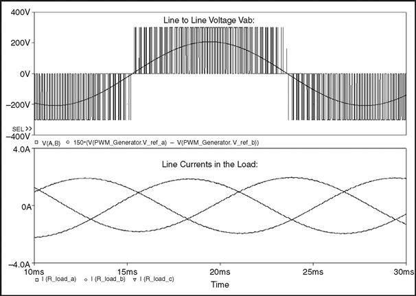
FIGURE 43.6 Output waveforms of the three-phase inverter with MOSFETs.
Figure 43.7 shows an example where the MOSFETs in Fig. 43.4 have been replaced with insulated gate bipolar transistor (IGBT). The particular IGBT shown here is included in the library of the evaluation version. Note that free-wheeling diodes are needed, if IGBTs are used. The free-wheeling diodes carry the load current when the IGBTs are turned off to provide a continuous path for the current. This is very important, since the load can have a substantial inductive component. Whenever the diodes are conducting, energy flows momentarily back to the source. In the case of power MOSFETs, the diodes (often called body diodes) are an integral part of the device. In the symbol graphic of PSpice® these body diodes are not shown for MOSFETs. For this circuit, the gate-drive circuit and the results are the same as for the three-phase bridge with power MOSFETs.
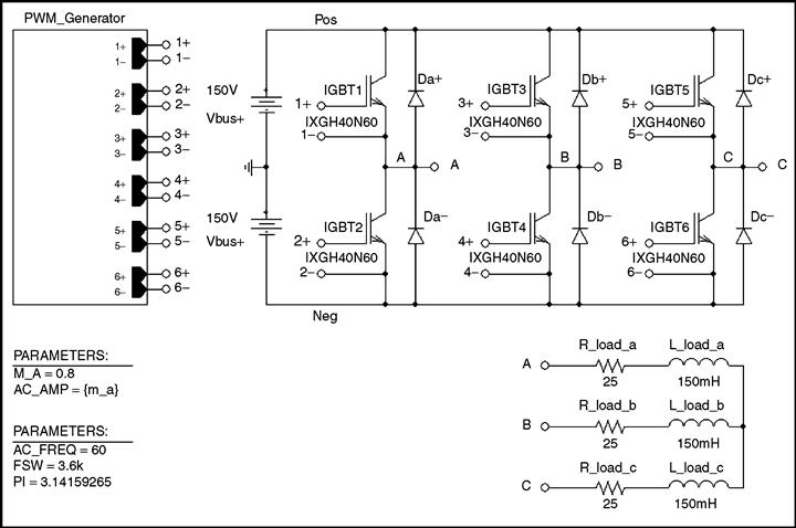
FIGURE 43.7 Three-phase inverter circuit with IGBTs.
43.4 Simulations of Power Electronic Circuits and Electric Machines
In the following, the start-up of an induction motor, fed by the three-phase inverter shown in Fig. 43.4, is presented. For this purpose, the simple passive load in Fig. 43.4 is replaced by an induction motor. For this and further discussions, it is assumed that the reader is familiar with the theory of induction machines. A number of excellent references are given at the end of this chapter [2, 3, 6, 7]. The induction motor symbol represents the electro-mechanical model of an induction motor. The model is suitable for studies of electrical and mechanical transients as well as steady-state conditions. The output pin on the motor shaft represents the mechanical output. The voltage on this pin represents the mechanical angular velocity using the relation 1V = 1 rad/s. In addition, any current drawn from or fed into this terminal represents applied motor or generator torque according to the relation 1A = 1 Nm. Due to these definitions, the electrical power associated with the voltage of the motor shaft (with respect to ground) is identical to the mechanical power. Following the well-known theory, the induction motor model has been derived for a two-phase (direct and quadrature, D, Q) equivalent motor. Attached to the motor is a bidirectional two-phase to three-phase converter module. This module is voltage and current invariant. This means that the voltage and current levels in the two-phase and the three-phase machine are equal. Consequently, the power in the two-phase machine is only two third of the power in the three-phase circuit. This is accounted for in the calculation of the electromagnetic torque (factor 3/2; see Eq. (43.4)). The internally generated torque can be monitored on the output labeled “Torque” on top of the sleeve around the motor shaft. The linear load in Fig. 43.8 is a symbol that represents an appropriately sized resistor to ground.
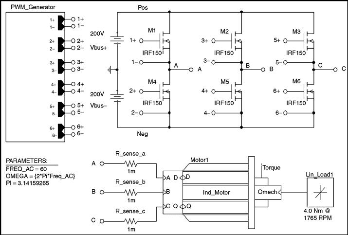
FIGURE 43.8 Induction motor start-up with three-phase inverter circuit.
In Fig. 43.8 the motor is represented by a custom symbol called “Motor1.” A simple hierarchical block could have been used for the motor, but a custom symbol has been created to achieve a more realistic and pleasing graphical representation. The symbol can be easily created with the symbol editor, which is built into the regular schematics (capture) editor. The editor provides standard graphical elements (lines, rectangles, circles etc.) so that professional looking symbols can easily be created. More details on this are shown in Figs. 43.19 and 43.20 and the accompanying discussion. Parameters are passed onto the subcircuit by using the name of the parameter preceded by a ‘@’ symbol. The advantage of passing parameters to subcircuits in this way is that several symbols can call one set of subcircuits with different parameters.
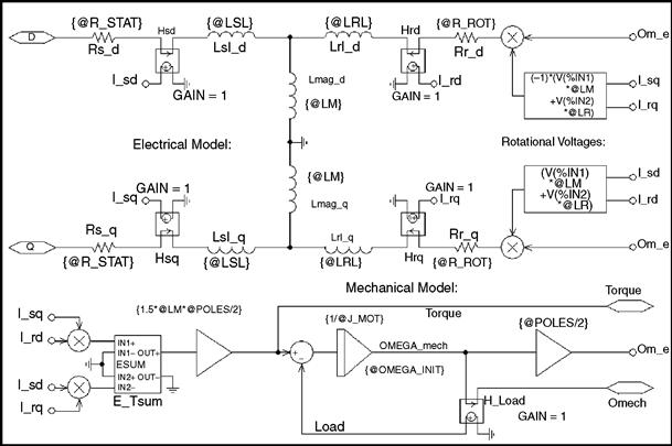
FIGURE 43.9 Subcircuit for induction motor model.
Right-clicking on the motor symbol and selecting “Descend Hierarchy” reveals the associated subcircuit that implements its function. This subcircuit is shown in Fig. 43.9. The upper portion of this subcircuit represents the electrical model. The task of the electrical model is to calculate the stator and rotor currents, with the stator voltages and the mechanical speed of the machine being input parameters. However, it is also possible without any changes, to feed stator currents (with controlled current sources) into the D and Q inputs and have the model to calculate the appropriate stator voltages. This option is useful for vector control applications, which are discussed later.
The equation system for the electrical model of a two-phase induction machine is given by Eq. (43.3). The theory for this equation system is derived in [2, 3, 6, 7]. The equation system and the model are formulated for the stationary reference frame. This reference frame assumes that the frame of the machine is stationary (which is hopefully the case in a real machine!) and the voltages and currents of the rotor are equivalent AC values with stator frequency. From machine theory we know that the actual rotor currents have slip frequency. Another reference frame is the synchronous (also called excitation) reference frame. In this reference frame, the stator of a fictitious machine is assumed to rotate with synchronous speed. The advantage of this reference frame is that the input frequency is zero (DC), which makes it easy to explain the principle of vector control by extending the theory of DC machines to AC machines.
 (43.3)
In typical implementations of vector control using digital signal processors (DSPs), the synchronous reference frame is used internally to calculate the reference values for the currents in the D and Q axis. These values are then transformed to the stationary reference frame in an additional step. Sometimes still other reference frames are used and it is possible to generate a universal electrical model with a reference frame speed input. This model could then be used for any reference frame.
The electrical model in Fig. 43.9 implements the equation system shown in Eq. (43.3). The circuit closely resembles the well-known T-equivalent circuit for the steady-state analysis of induction machines. Two instances of the T-equivalent circuit are necessary to implement the two-phase (D, Q) model. The two instances of the circuit are almost mirror images of each other (and actually drawn that way) except for some differences in the circuit elements that calculate the voltages, which are generated due to the rotation of the rotor. The bottom of Fig. 43.9 represents the mechanical model. This circuitry calculates the internally generated electro-magnetic torque, using the rotor and stator currents as input values. The equation for the internal electromagnetic torque of the induction machine is given by Eq. (43.4) [3, 6, 7]. The factor 3/2 accounts for the fact that the real motor is a three-phase machine. Using the generated torque, the load torque, and the moment of inertia, the angular acceleration can be calculated. Integration of the angular acceleration yields the rotor speed, which is used in the electrical model. To avoid clutter and to improve readability, connection bubbles are used to connect the various parts of the model together.
![]() (43.4)
(43.4)
Since typical induction machines are three-phase machines, it is often desirable to have a machine model with a three-phase input. Therefore, a bidirectional two-phase to three-phase converter module, which can be attached to the motor, has been developed. A subcircuit for this module is shown in Fig. 43.10. This circuit is truly bidirectional, meaning that the circuit can be fed with voltage or current sources from either side. The equation system for this voltage and current invariant transformation is given by Eq. (43.5). This transformation is sometimes called “Clark” or “ABC-DQ” transformation. Note that V0 denotes a zero-sequence voltage, which is assumed to be zero. This voltage would only have non-zero values for unbalanced conditions. An interesting detail of the subcircuit is the three-phase switch on the input. This switch is necessary to ensure a stable initialization of the simulator in case the machine is fed with a controlled current source. The switch provides an initial shunt resistor from the three-phase input to ground. Soon after the simulation has started, the switch opens and leaves only a negligible shunt conductance to ground.
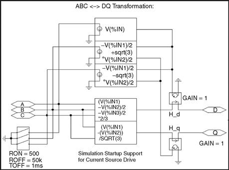
FIGURE 43.10 Subcircuit for the ABC-DQ transformation module.
 (43.5)
Figure 43.11 shows the result for the start-up of the induction motor for the circuit of Fig. 43.8. The motor is a half (Attention LE(½)) hp, 208V, 4-pole machine. The detailed parameters are shown in Table 43.1. The PWM generation was identical to the example shown in Fig. 43.4, except that the switching frequency was 4 kHz and 21.1% of the third harmonic has been added to each of the reference sinusoids in order to increase the linear modulation range. The resulting reference waveform was then multiplied with 1.14, which represented the maximum voltage for linear modulation. The top trace in Fig. 43.11 shows the developed electromagnetic torque, the level for the rated steady-state torque (4 Nm as commanded by the load in Fig. 43.8) and the zero level. This graph shows the typical oscillatory torque production of the induction machine for an uncontrolled line start. The scale for this graph is 1V = 1 Nm. The graph below shows the mechanical angular velocity with a scale of 1V = 1 rad/s. Below the graph for the rotor speed, all three input currents are shown. It is evident, that the current traces are almost perfect sinusoids, despite the fact that the input voltage is the PWM waveform shown in the bottom graph. Also, the trace for the torque shows no discernable high frequency ripple. The reason is, of course, that the motor windings are inductive, and represent a low-pass filter for the applied voltages. Nevertheless, recent research suggests that filtering the output voltage of the inverter is advantageous anyway, because it significantly reduces the voltage stress on the windings and suppresses displacement currents through the bearings [8].
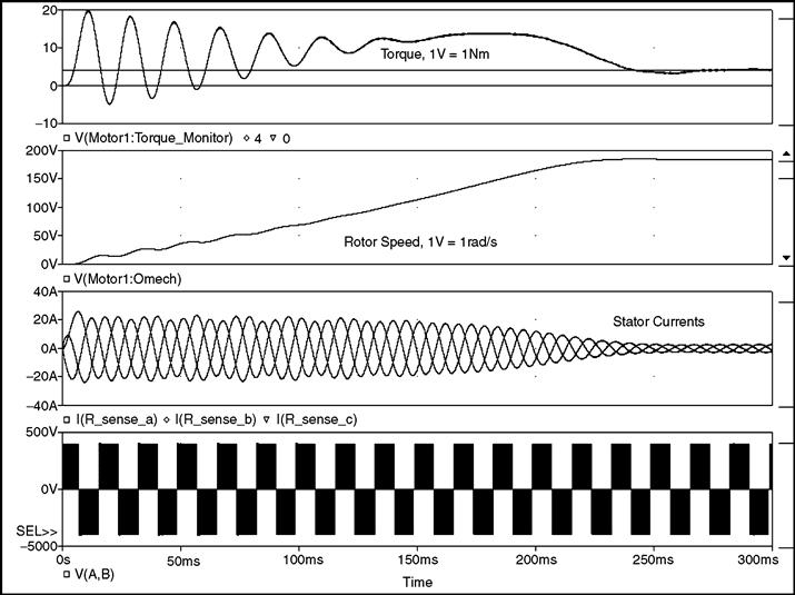
FIGURE 43.11 Induction motor start-up with three-phase inverter circuit.
TABLE 43.1 List of all attributes used for the half (Attention LE:(½)) hp, 208 V, four-pole induction motor in Fig. 43.8
| Attributes: |
| PART = Induction_Servo |
| MODEL = Ind_Motor |
| TEMPLATE = |
| J_mot = 0.01 |
| Omega_init = 0.0 |
| Ls = (@Lm + @Lsl) |
| Lr = (@Lm + @Lrl) |
| Poles = 4 |
| Tau_r = (@Lr/@R_Rot) |
| REFDES = Motor? |
| Lsl = 14.96mH |
| Lrl = 8.79mH |
| R_Stat = 3.60 |
| R_Rot = 1.90 |
| Lm = 424.41mH |
43.5 Simulations of AC Induction Machines Using Field Oriented (Vector) Control
The following examples will demonstrate the use of PSpice® for simulations of AC induction machines using field oriented control (FOC). Again, it is assumed that the reader is familiar with the basics of induction machine theory. Often times, FOC is also called vector control, and both expressions can be used interchangeably. The FOC was proposed in the 1960s by Hasse and Blaschke, working at the Technical University of Darmstadt [9]. The basic idea of FOC is to inject currents into the stator of an induction machine such that the magnetic flux level and the production of electromagnetic torque can be independently controlled and the dynamics of the machine resembles that of a separately excited DC machine (without armature reaction; no cross coupling). The previously discussed two-phase model for the induction machine is very helpful for studies of vector control and shall be used in all examples. If a two-phase induction motor model for the synchronous (or excitation) reference frame is used, the similarities between the control of a separately excited DC machine and vector control of an AC induction machine would be most evident. In this case, the D input would correspond to the field excitation input of the DC machine and both inputs would be fed with DC current. Assuming unsaturated machines, the current into the D input of the induction machine or the field current in the DC machine would control the flux level. The Q input of the induction machine would correspond to the armature winding input of the DC machine and again both inputs would receive DC current. These currents would directly control the production of electromagnetic torque with a linear relation (constant kT) between the current level and the torque level. Furthermore, the Q component of the current would not change the flux level established by the D component (no cross coupling). To make such a simulation work, it would finally be necessary to calculate the slip value that corresponds to the commanded torque and supply this DC value to the D, Q (synchronous reference frame) machine model.
Of course this is very interesting from an academic standpoint and the author uses this example in a semester long lecture on FOC. However, it should again be noted, that a machine represented by a model with a synchronous reference frame would have a stator, which rotates with synchronous speed. Of course this is not realistic and therefore it is more interesting to generate a simulation example that uses the previously discussed motor with a model for the stationary reference frame. This motor must be supplied with AC voltages and currents with a frequency determined mostly by the rotor speed to a small extent by the commanded torque. We still supply DC values representing the commanded flux and torque but we transform these DC values to appropriate AC values. In the following example, we will assume that we can measure the actual rotor speed with a sensor. This can, in effect, be easily accomplished and many types of sensors are available on the market. If we add the slip speed, that we determine mathematically from the torque command, to the measured rotor speed, we obtain the synchronous speed for the given operating point. With this synchronous speed we can transform the DC flux and torque command values from the synchronous reference frame to the stationary reference frame. We accomplish this by using a rotational transformation according to the matrix equations in Eq. (43.6). This rotational transformation is also called “Park” transformation.
 (43.6)
As shown in Eq. (43.6), the transformation is bidirectional and the product of the transformation matrices yields the unity matrix. For the following discussion we shall define the transformation, which produces AC values from DC inputs as a positive vector transformation and the reverse operation consequently a negative vector transformation. The matrix equation for the positive vector transformation is shown on the left side of Eq. (43.6). The negative transformation is very useful to extract DC values from AC voltages and currents for diagnostic and feedback control purposes. We will also make use of it for sensorless vector control, which is discussed below. Both rotational transformations use the angle, ρ, in the equations. This angle can be interpreted as the momentary rotational displacement angle between two Cartesian coordinate systems; one containing the input values and the other, the output values. This angle is obtained by integration of the angular velocity with which the coordinate systems are rotating (typically the synchronous speed).
In summary, we replaced a theoretical motor model using a synchronous reference frame by a reference frame transformation of the supply voltages and currents. In fact, modern DSPs like the TMS320C2000™ Digital Signal Controller series from Texas Instruments are capable to perform both the Clark and the Park transformation in both directions at very high speeds [10]. These DSPs are well supported with proven reference designs, including free software examples.
Figure 43.12 shows the top level of a simulation example that implements vector control for an induction machine with a stationary reference frame model. In fact, the motor model and the associated subcircuits are identical to the ones used for the circuit shown in Fig. 43.8. However, a more powerful motor is used here, specifically a 3 hp, 4-pole 208 V motor with circuit parameters shown in Table 43.2. As discussed above, the actual speed of the rotor is used as an input signal for the control unit. This scheme is known as indirect vector control and represents one of the most often used arrangements. The symbol for the controller has the same parameters as the motor. This is necessary to achieve correct field orientation. In real systems, the controller also must know or somehow determine the machine parameters. The machine parameters could have also been established globally using “PARAM” symbols, but if the parameters for the controller can be set separately as it is the case here, the influence of parameter mismatch on the performance of the control can be easily studied. An example of this is given in Fig. 43.12.
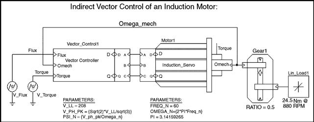
FIGURE 43.12 Top level circuit for indirect vector control of induction motors.
TABLE 43.2 List of all attributes for the induction motor symbol for vector control
| Attributes: |
| PART = Induction_Servo |
| MODEL = Ind_Motor |
| TEMPLATE = |
| J_mot = 0.1 |
| Omega_init = 0.0 |
| Ls = (@Lm + @Lsl) |
| Lr = (@Lm + @Lrl) |
| Poles = 4 |
| Tau_r = (@Lr/@R_Rot) |
| REFDES = Motor? |
| Lsl = 2.18mH |
| Lrl = 2.89mH |
| R_Stat = 0.48 |
| R_Rot = 0.358 |
| Lm = 51.25mH |
Figure 43.12 also shows a symbol for a mechanical gear, which is attached to the output of the induction motor. Let us recall that the voltage on the mechanical output terminal represents the angular velocity and the current represents the torque. We also know that the product of the angular velocity and the torque is the mechanical power. Therefore it is easily understood that the electrical representation of an ideal gear is an ideal transformer. The ideal transformer changes speed (voltage) and torque (current) just like an ideal gear. Also there are no power losses in an ideal transformer as well as in an ideal gear.
In this fashion, many more mechanical properties and devices can be modeled. For example, a mechanical flywheel is simply represented by a capacitor to ground. Due to the scaling factors for the angular velocity and the torque, a flywheel with J = 1 kgm2 would be a capacitor with C = 1F. The compliance of a drive-shaft (elastic twisting by the applied torque) can be modeled by a series inductor. By including both capacitors and inductors, effects like mechanical resonance can be included in a model.
Figure 43.13 shows the subcircuit for the vector control unit. The central part is a vector rotator for positive direction. This element transforms the DC reference values for the flux (D-axis) and the torque (Q-axis) to the stationary reference frame. The input angle for the vector rotator is the integral of the synchronous angular velocity. The signal called “Omega_o” is the measured rotor speed.
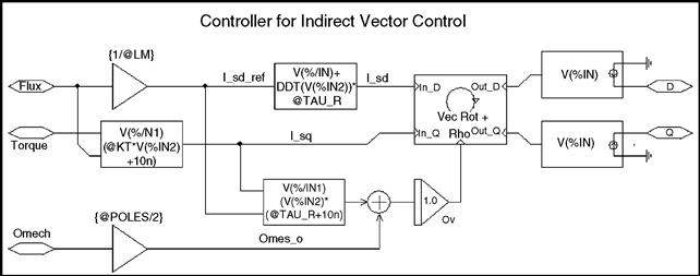
FIGURE 43.13 Subcircuit for indirect vector control of induction motors.
This speed is multiplied with the number of pole-pairs (poles/2) to obtain the electrical angular velocity. Then the slip value (see Eq. (43.7) for slip frequency calculation for vector control) appropriate to the torque command is added and the resulting signal is routed through an integrator to generate the input angle for the vector rotator.
In the D-axis, a differentiator function “DDT()” is used in a compensation (see Eq. (43.8) for D-axis reference current for vector control) element which assures that the actual flux in the machine follows the commanded signal without delay. The input and output values of the vector rotator are voltage signals which correspond 1:1 to current signals. (In a real controller the currents are typically scaled values in the memory of a DSP.) In fact, the vector controller calculates the appropriate currents that need to be injected into the machine to perform as desired. Two voltage-controlled current sources with unity gain are connected to the output of the vector rotator to generate these currents. In a real system, the controlled current sources are realized by an inverter with current feedback. In the most realistic case, this would be a three-phase inverter and the ABC-DQ transformation would be performed before the current controlled inverter. In this example, the ABC-DQ transformation has been performed outside the controller and the motor. This way, it is possible to study vector control principles using a DQ controller and a DQ motor by eliminating the ABC-DQ transformation elements. An example is given in Fig. 43.14.
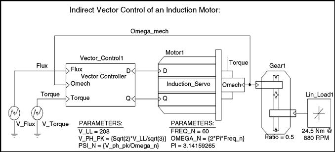
FIGURE 43.14 Circuit for indirect vector control without ABC-DQ transformations.
![]() (43.7)
(43.7)
Figure 43.15 shows the results obtained for the circuit shown in Figs. 43.12 and 43.14 with perfect tuning of the vector controller. Perfect tuning means that the controller precisely knows all motor parameters at all times (including resistance changes due to heating of the windings). The two traces in the diagram on top of Fig. 43.15 represent the traces for the D and Q input signals of the vector rotator. The graph below shows the reference value for the flux. It is evident, that the flux level is being changed at the same time when 10 Nm of torque is commanded (and produced). This is done to check if the torque and the flux can be independently controlled, which is true for correct FOC. Below the flux reference is the graph for the mechanical angular velocity. It can be seen, that the machine accelerates whenever torque is developed and slows down due to the load when the torque command is driven to zero. The graph on the bottom of Fig. 43.15 provides the easiest way to judge the quality of the correct field orientation. This graph shows the traces of the commanded and the actually produced torque and in this case they are perfectly on top of each other at all times.
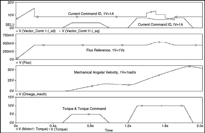
FIGURE 43.15 Results for indirect vector control with perfect tuning.
Figure 43.16 is an example of the results obtained from a de-tuned vector controller. The circuit is identical to the circuit in Fig. 43.12, except for the fact that the rotor resistance value in the controller was increased to 125%, which is thought to be attributed to heating of the rotor bars. It is obvious that the traces for the commanded and the actually produced torque are no longer identical. This is especially true, during times when the flux is changing. De-tuning is actually a real problem in industrial vector control applications. De-tuning is caused by the fact that the machine parameters are not precisely known to begin with and/or, are changing during the operation of the machine. The values of the winding resistance are most likely to change due to heating of the machine.
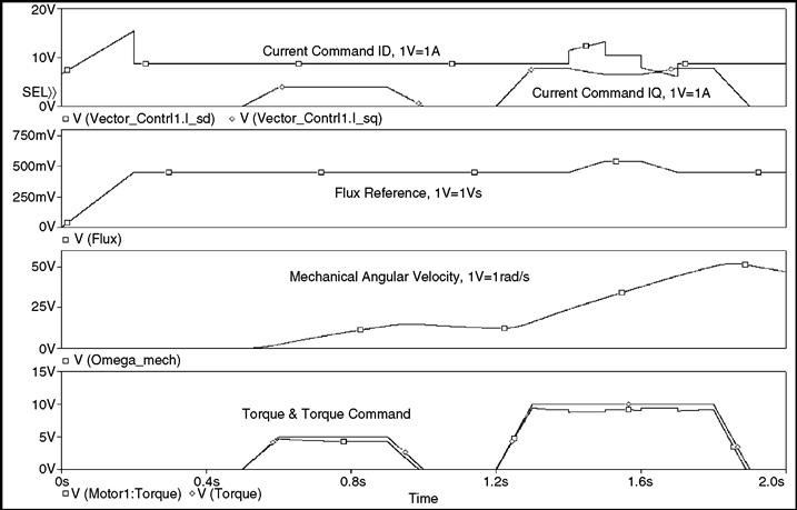
FIGURE 43.16 Results for indirect vector control with 125% rotor resistance.
43.6 Simulation of Sensorless Vector Control Using PSpice®
In the previous example, the advantages of vector control have been shown. However, for the implementation of the control scheme a sensor for the mechanical speed was necessary. This could pose a problem for applications, where a vector control unit is to be retrofitted into existing equipment. The motor installation may not easily allow the installation of a mechanical speed sensor. Therefore engineers have thought to replace the mechanical speed sensor with a speed observer, which is a mathematical model that is evaluated by the control processor (typically a DSP), which is performing the standard vector control computations anyway. The algorithm for the observer would use the measured stator voltages and currents for the D- and Q-axes as input parameters. It would also rely on the knowledge of the machine model and on the correct machine parameters (rotor and stator resistance, mutual and leakage inductance, etc.). The following example shows such an arrangement. It could be derived from the previous example with the only difference being that the speed sensor signal is replaced by a speed observer. However, careful examination of the derivation [2] of the speed observer reveals, that it is easier to calculate the synchronous angular velocity, which is ultimately desired anyway, than the angular velocity of the rotor. Therefore, the observer was modified and the calculation of the rotor speed and the subsequent addition of the slip speed was foregone. The speed observer used here basically solves the D, Q equation system of the induction machine shown in Eq. (43.3), with the only difference that some of the dependent variables are now independent and vice versa. In addition to the synchronous angular velocity, the observer provides the values of the rotor flux, which are used in the D-axis signal path. The advantage of this is that the compensator with the differentiation function, which is problematic from a numerical stability standpoint, can be eliminated.
Figure 43.17 shows the top level of a simulation project for sensorless vector control. The top view of this circuit is very similar to the circuit for the indirect vector control represented by Figs. 43.12 and 43.14 except for the missing motor-speed feedback. The model for the motor and the motor's parameters are precisely the same as in the example for the indirect vector control. Selecting the “Sensorless Vector Control” block and choosing “Descend Hierarchy” reveals the associated subcircuit, which is shown in Fig. 43.18. This subcircuit is similar to the subcircuit for the indirect vector control with two exceptions: first and foremost, the motor-speed feedback signal is replaced by the speed observer. In this case the speed observer directly provides the synchronous angular velocity. Therefore, it is not necessary to calculate the slip speed and add it to the rotor speed to obtain the synchronous speed. Second, the values of the rotor flux, which are available from the speed observer, are used to calculate the reference value for the torque producing current (Q) component. Therefore, the compensation term, which contains a differentiator in the D-axis of the controller shown in Fig. 43.13 can be eliminated. The purpose of the compensation term is to ensure that the flux is equal to the flux command at all times with no delay. If that is assured, the command signal can be chosen in place of the real flux to calculate how much torque producing current is necessary to obtain the desired torque.
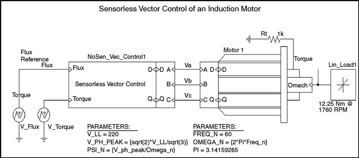
FIGURE 43.17 Top level of simulation circuit for sensorless vector control.
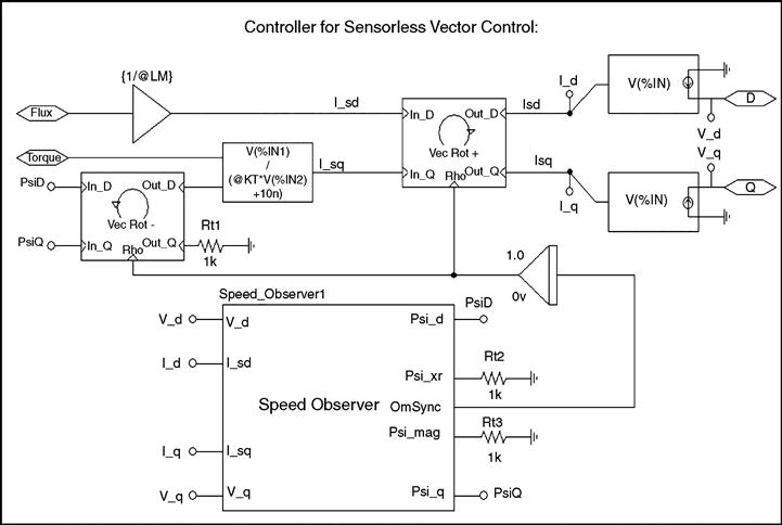
FIGURE 43.18 Subcircuit for sensorless vector controller.
In order to demonstrate how to obtain a more compact motor model, the extensive subcircuit of the induction motor model (see Fig. 43.9) has been replaced by a number of additional attributes which have been added to the motor symbol using the symbol editor.
However, if the actual flux is known (observed), this value can be used instead. Since the flux observer is fed by the D- and Q-axes voltages and currents for the stationary reference frame, the flux components need to be transformed back into the synchronous reference frame. This is done with the “Negative Vector Rotator” located above and to the left of the speed observer in Fig. 43.18.
The easiest way to start the symbol editor and to open the appropriate library is to select the symbol by clicking into it and then select the “Edit Symbol” function. The additional attributes of the modified motor symbol will enter the equivalent to the subcircuit represented by Fig. 43.9 into the netlist. The netlist is a compilation of the schematic pages into a textual description in ASCII format. From a usability standpoint, a “self-contained” symbol like this is a very elegant solution, since the file for the subcircuit is no longer required.
Since the PSpice® simulation engine always uses the netlist as the input, the circuit works identically. For the PSpice® simulation it makes no difference, where the netlist or part of it comes from. This also means that even the most recent release of PSpice® can still simulate legacy files that have been created before the introduction of schematic editors. The introduction of netlist entries is done via the “TEMPLATE” attribute. This attribute is a system attribute and a part of every symbol. Therefore, the TEMPLATE attribute is of course present in the attribute list for the motor symbols in the previous examples. These attribute lists are shown in Tables 43.1 and 43.2. In these tables the TEMPLATE attribute has no value since the netlist entries are made by the symbols in the associated subcircuit. To give a reader a better understanding of the self-contained machine symbol, the format of some common netlist entries and the syntax of the value of the TEMPLATE attribute is discussed. It is also very helpful to examine the TEMPLATE attributes of existing symbols.
Figure 43.19 shows the screen view of the symbol for the induction motor in the symbol editor in PSpice®/Cadence Release 9.1, which was used for the development of this part. Figure 43.20 shows a similar view; however, here the window for entry and editing of attributes is also visible. This screen can be invoked using the “Options/Part Properties…” dialog.
The format of the netlist entries for some common elements is:
[] denotes space holder for name extension specific for a symbol to avoid duplicate names.
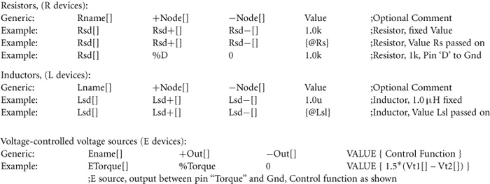

FIGURE 43.19 Screen view of motor symbol in the symbol editor.
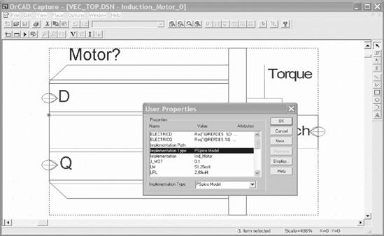
FIGURE 43.20 Screen view of symbol editor with user properties input window.
The attributes, that create the netlist entries, which insert the previously discussed model for the motor are entered here. A complete list of all attributes, extracted from a working example, is given in Table 43.3. Therefore, the reader should be able to enter the attributes exactly as printed and obtain a working model.
TABLE 43.3 List of all attributes used for the self-contained induction motor symbol
| Attributes: |
| REFDES = Motor? |
| PART = Ind_Motor |
| MODEL = Ind_Motor |
| TEMPLATE = @ElectricD @ElectricQ @Mechanical |
| R_Stat = 0.48 |
| R_Rot = 0.358 |
| Lm = 51.25mH |
| Lsl = 2.18mH |
| Lrl = 2.89mH |
| J_mot = 0.1 |
| Omega_init = 0.0 |
| Poles = 4 |
| ElectricD = Rsd |
|
Lsld |
|
Lmd |
|
Lrld |
|
Rrd |
|
Erotd |
|
+ +(V(ErotQ |
| ElectricQ=Rsq |
|
Lslq |
|
Lmq |
|
Lrlq |
|
Rrq |
|
Erotq |
|
+ +(V(ErotD |
| Mechanical=ETorque |
| + VALUE { (1.5*@Lm*@Poles/2) * ( |
|
+ ((V(%Q, 3 |
|
+ ((V(%D, 1 |
|
EOme |
|
VLd |
| @Omega_init} |
According to Table 43.3, the value for the TEMPLATE attribute is as follows:
TEMPLATE = @ElectricD @ElectricQ @Mechanical
This statement will insert the expression for “ElectricD,” i.e. the T-equivalent circuit for the D-axis, two carriage returns “ ,” the expression for “ElectricQ,” i.e. the T-equivalent circuit for the Q-axis, two more carriage returns “ ,” and finally the expression for “Mechanical,” i.e. the mechanical model into the netlist. The expressions for “ElectricD,” “ElectricQ,” and “Mechanical” are defined in separate attributes. Careful examination of the values of the “ElectricD,” “ElectricQ,” and “Mechanical” attributes reveals a number of repetitive terms. The meaning of these terms are explained below:
| @Name | –Substitutes what is defined for “@Name” at the current place. |
| –Inserts the path “ | |
| –new line (carriage return) is inserted into the netlist, however the value of the attribute does not have a carriage return in it. This means everything listed after “ElectricD” until “ElectricQ” goes on one line. If the symbol definition is printed however, it is shown as in Table 43.3. | |
| + | –new line and continuation of expression. |
| + + | –new line, continuation of expression, numerical operator “+.” |
Figure 43.21 shows a subcircuit for the speed observer. This schematic shows the structure and all the details of the implementation in the form of a block diagram. The speed observer uses the stator voltages and currents for the D- and the Q-axis as input variables. After subtracting the voltage drop across the winding resistance and the leakage inductance of the stator from the stator input voltage and scaling the result by Lr/Lm, the observer calculates the D and Q components of the rotor flux by integration. Since the input values are in the stationary reference frame, so are the results. The observer also calculates the magnitude of the rotor flux (Eq. (43.9)) and then calculates the synchronous angular velocity (Eq. (43.10)) by evaluating the rate of change of the ratio of the D and Q components. The mathematical relationships are given by the Eqs. (43.9) and 43.10 [2].
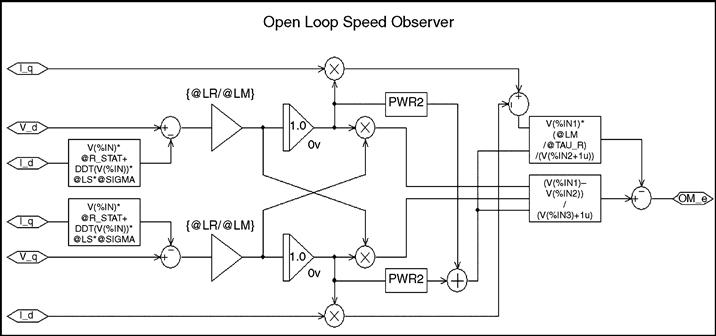
FIGURE 43.21 Subcircuit for speed observer for sensorless vector controller.
 (43.9)
 (43.10)
Since the observer shown in Fig. 43.21 has a large number of elements, this subcircuit has also been integrated into a custom part by creating an appropriate TEMPLATE and other supporting attributes. A complete listing, which was extracted from thoroughly tested part, is given in Table 43.4. Using this table, the reader should be able to create this very complex part with relative ease.
TABLE 43.4 List of all attributes for the speed observer symbol
| Attributes: |
| REFDES = Speed_Observer? |
| PART = Speed_Obs |
| MODEL = Speed_Obs |
| TEMPLATE = Ed |
| + @EXP_d2 + @EXP_d3 } |
|
Eq |
| + @EXP_q2 + @EXP_q3 } |
|
Emag |
|
Exr |
| + @EXP_x2 + @EXP_x3 + @EXP_x4 } |
|
EOmSync |
| SIMULATIONONLY = |
| EXP_d1 = @Ini_d + |
| EXP_d2 = SDT((@Lr/@Lm)*(V(%V_d) - V(%I_sd)*@R_Stat |
| EXP_d3 = -DDT(V(%I_sd))*@Ls*@Sigma)) |
| EXP_q1 = @Ini_q + |
| EXP_q2 = SDT((@Lr/@Lm)*(V(%V_q) - V(%I_sq)*@R_Stat |
| EXP_q3 = -DDT(V(%I_sq))*@Ls*@Sigma)) |
| Ini_d = 0.0V |
| Ini_q = 0.0V |
| EXP_x1 = (V(%Psi_d)*(@Lr/@Lm)* |
| EXP_x2 = (V(%V_q) - V(%I_sq)*@R_Stat - DDT(V(%I_sq))*@Ls*@Sigma)) |
| EXP_x3 = -(V(%Psi_q)*(@Lr/@Lm)* |
| EXP_x4 = (V(%V_d) - V(%I_sd)*@R_Stat - DDT(V(%I_sd))*@Ls*@Sigma)) |
| EXP_om1 = (V(%Psi_xr)/(V(%Psi_mag) + lu)) |
Figure 43.22 shows the output for the speed sensorless vector control project as it presents itself in the PSpice® 9.1/ORCAD evaluation version.
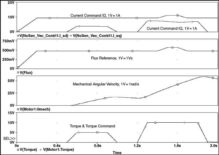
FIGURE 43.22 Simulation results for sensorless vector control.
A comparison of the traces for the torque and the torque command (they are perfectly on top of each other) shows that the scheme works extremely well. It even works for a start from zero speed, which is typically not the case in real systems. The reason is, that the uncertainties of the winding resistance values (note that they change with temperature) create errors in observers like this one. The problem is worst at low speeds, because at low speeds and associated low stator frequencies, the uncertain winding resistance represents the largest part of the total machine impedance.
43.7 Simulations Using Simplorer®
In the following, some examples of simulations with the evaluation version of Simplorer® [11], Release 4.1 are shown. It should be acknowledged at this point that these examples have been created by Ali Ricardo Buendia, who obtained M.S.E.E degree from Texas Tech University. The advantages of Simplorer® are that it has a lot of models for power electronics devices and machines built-in, since it is specialized for this type of simulation. Also, no numerical convergence problems have been noticed thus far. Figure 43.23 shows the schematic for a three-phase diode rectifier. The input is a balanced three-phase source with a reactive source impedance. An exponential characteristic, closely resembling real diodes, has been chosen as a model for the diodes.
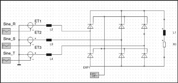
FIGURE 43.23 Simplorer® schematics for three-phase rectifier.
Figure 43.24 shows a circuit, which transforms the load currents from a three-phase to a two-phase system. Here the D and Q components are called alpha and beta components respectively. The results of the simulation are shown on the same page that is used for the schematic diagrams shown by the previous two figures. Figure 43.25 shows a plot of the line currents during the start-up of the rectifier, where the initial load current is zero. The next graph shows a plot of the line currents that have been transformed by the circuit shown in Fig. 43.26. The components of the line currents are the variables of the axes. The plot shows the typical hexagonal trace that can be expected for this type of line-commutated rectifier (six step operation). If the converted source voltages were plotted in this fashion, a perfect circle would be the result.
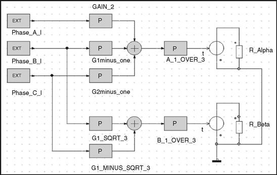
FIGURE 43.24 Three-phase to two-phase conversion for load currents.
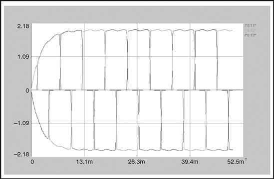
FIGURE 43.25 Simplorer® plot of load currents for the three-phase rectifier.
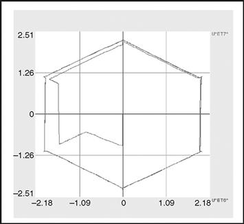
FIGURE 43.26 Plot of converted load currents for the three-phase rectifier.
The last two graphs demonstrate a Simplorer® simulation of the start of an induction motor. As previously mentioned, the symbol and the model for the induction motor is built into the code. Figure 43.27 shows the schematic with the source and the induction motor as well as a graph that shows the rotational speed as a function of time. The graph below shows plots of the stator and rotor flux components, which are available from the machine model. Like the plot of the current components for the rectifier, the flux components are the variables of the axes in the graphs of Fig. 43.28.
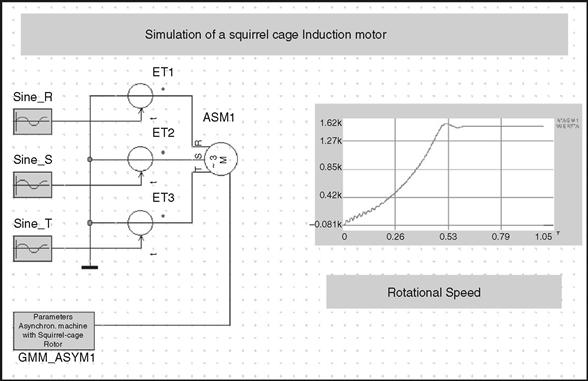
FIGURE 43.27 Simplorer® schematics for induction motor start.
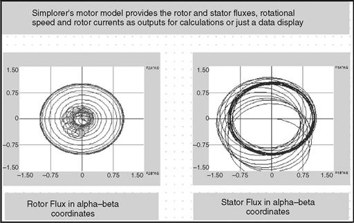
FIGURE 43.28 Simplorer® plots of machine fluxes for induction motor start.
43.8 Conclusions
In this chapter, the capabilities of PSpice® [12] and Simplorer® [11] have been used to simulate a number of projects from the power electronics, machines, and drives area. The advantage of PSpice® is that it is based on the almost universal Spice simulation language, which can be seen as the worldwide de facto standard. On the other hand, Simplorer® has the advantage of built-in machine models. If both programs are used, comparisons and mutual validations of models can be performed. The reader should always validate any model before it is used for critical engineering decisions. It was pointed out in the introduction, that model validation often means verification that the limitations of the model are not exceeded.
In addition to the detailed examples, some general guidelines on the uses of simulation for analysis and design have been developed. All tested programs yielded excellent results. The simulation time for each project shown is typically less than a minute on a typical (2005) PC. The author hopes, that the reader has gotten an insight and appreciation of the power of these modern simulation codes and some useful ideas and inspirations for projects of his own.
REFERENCES
1. Mohan N, Undeland T, Robbins W. Power Electronics, Converters, Applications, and Design. 2nd edition New York: John Wiley & Sons; 1995.
2. Trzynadlowski AM. The Field Orientation Principle in Control of Induction Motors. Boston, MA: Kluwer Academic Publishers, Inc.; 1994.
3. Krause PC, Wasynczuk O, Sudhoff SD. Analysis of Electric Machinery. Hoboken, NJ: IEEE Press; 1995.
4. Giesselmann MG. Averaged and Cycle by Cycle Switching Models for Buck, Boost, Buck-Boost and Cuk Converters with common Average Switch Model. Proceedings of the 32nd Intersociety Energy Conversion Engineering Conference. 1997; 01.
5. Giesselmann M. A PSpice® Tutorial for Demonstrating Digital Logic. IEEE Transactions on Education. Nov. 1999; [http://coeweb.engr.unr.edu/eee/59/CDROM/Begin.htm].
6. Novotny DW, Lipo TA. Vector Control and Dynamics of AC Drives. New York, NY: Oxford Science Publications; 1996.
7. Vas P. Vector Control of AC Machines. Oxford Science Publications 1990.
8. Von Jouanne A, Rendusara D, Enjeti P, Gray W. Filtering Techniques to Minimize the Effect of Long Motor Leads on PWM Inverter Fed AC Motor Drive Systems. IEEE Transactions on Industry Applications. July/Aug. 1996; 919–926.
9. K. Hasse, “Zur Dynamik Drehzahlgeregelter Antriebe mit Stromrichter gespeisten Asynchron-Kurzschlussl′ ‘aufermachinen,” (On the Dynamics of Adjustable Speed Drives with converter-fed Squirrel Cage Induction Machines), Ph.D. Dissertation, Technical University of Darmstadt, 1969.
10. ACI3_4: Sensor-less Direct Flux Vector Control of 3-phase ACI Motor, Data Sheet, Texas Instruments Incorporated, 12500 TI Boulevard, Dallas, TX 75243-4136, 800-336-5236.
11. Simplorer®, Technical Documentation, Ansoft Corporate Headquarters, 225 West Station Square Drive, Suite 200, Pittsburgh, PA 15219, USA, (412) 261-3200, http://www.ansoft.com/products/em/simplorer/.
12. PSpice® Documentation, 2655 Seely Avenue, San Jose, California 95134, USA, (408) 943-1234, http://www.cadence.com/.