5

Load–Strength Interference

5.1 Introduction

In Chapter 1 we set out the premise that a common cause of failure results from the situation when the applied load exceeds the strength. Load and strength are considered in the widest sense. ‘Load’ might refer to a mechanical stress, a voltage, a cyclical load, or internally generated stresses such as temperature. ‘Strength’ might refer to any resisting physical property, such as hardness, strength, melting point or adhesion. Please note that the Load-Strength concept is often referred in the literature as ‘Stress-Strength’.

Examples are:

1. A bearing fails when the internally generated loads (due perhaps to roughness, loss of lubricity, etc.) exceed the local strength, causing fracture, overheating or seizure.
2. A transistor gate in an integrated circuit fails when the voltage applied causes a local current density, and hence temperature rise, above the melting point of the conductor or semiconductor material.
3. A hydraulic valve fails when the seal cannot withstand the applied pressure without leaking excessively.
4. A shaft fractures when torque exceeds strength.
5. Solder joints inside a vehicle radio develop cracks before the intended service life due to temperature cycling fatigue caused by the internal heating.

Therefore, if we design so that strength exceeds load, we should not have failures. This is the normal approach to design, in which the designer considers the likely extreme values of load and strength, and ensures that an adequate safety factor is provided.

Additional factors of safety may be applied, for example as defined in pressure vessel design codes or electronic component derating rules. This approach is usually effective. Nevertheless, some failures do occur which can be represented by the load-strength model. By our definition, either the load was then too high or the strength too low. Since load and strength were considered in the design, what went wrong?

5.2 Distributed Load and Strength

For most products neither load nor strength are fixed, but are distributed statistically. This is shown in Figure 5.1(a). Each distribution has a mean value, denoted by or , and a standard deviation, denoted by σ_L or σ_S. If an event occurs in which the two distributions overlap, that is an item at the extreme weak end of the strength distribution is subjected to a load at the extreme high end of the load distribution, such that the ‘tails’ of the distributions overlap, failure will occur. This situation is shown in Figure 5.1(b).

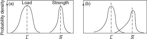
Figure 5.1 Distributed load and strength: (a) non-overlapping distributions, (b) overlapping distributions.

For distributed load and strength, we define two factors, the safety margin (SM),

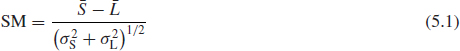
and the loading roughness (LR),

The safety margin is the relative separation of the mean values of load and strength and the loading roughness is the standard deviation of the load; both are relative to the combined standard deviation of the load and strength distributions.

The safety margin and loading roughness allow us, in theory, to analyse the way in which load and strength distributions interfere, and so generate a probability of failure. By contrast, a traditional deterministic safety factor, based upon mean or maximum/minimum values, does not allow a reliability estimate to be made. On the other hand, good data on load and strength properties are very often not available. Other practical difficulties arise in applying the theory, and engineers must always be alert to the fact that people, materials and the environment will not necessarily be constrained to the statistical models being used. The rest of this chapter will describe the theoretical basis of load-strength interference analysis. The theory must be applied with care and with full awareness of the practical limitations. These are discussed later.

Some examples of different safety margin/loading roughness situations are shown in Figure 5.2. Figure 5.2(a) shows a highly reliable situation: narrow distributions of load and strength, low loading roughness and a large safety margin. If we can control the spread of strength and load, and provide such a high safety margin, the design should be intrinsically failure-free. (Note that we are considering situations where the mean strength remains constant, i.e. there is no strength degradation with time. We will cover strength degradation later.) This is the concept applied in most designs, particularly of critical components such as civil engineering structures and pressure vessels. We apply a safety margin which experience shows to be adequate; we control quality, dimensions, and so on, to limit the strength variations, and the load variation is either naturally or artificially constrained.

Figure 5.2(b) shows a situation where loading roughness is low, but due to a large standard deviation of the strength distribution the safety margin is low. Extreme load events will cause failure of weak items. However, only a small proportion of items will fail when subjected to extreme loads. This is typical of a situation where quality control methods cannot conveniently reduce the standard deviation of the strength distribution (e.g. in electronic device manufacture, where 100% visual and mechanical inspection is seldom feasible). In this case deliberate overstress can be applied to cause weak items to fail, thus leaving a population with a strength distribution which is truncated to the left (Figure 5.3). The overlap is thus eliminated and the reliability of the surviving population is increased. This is the justification for high stress burn-in of electronic devices, proof-testing of pressure vessels, and so on. Note that the overstress test not only destroys weak items, it may also cause weakening (strength degradation) of good items. Therefore the burn-in test should only be applied after careful engineering and cost analysis.

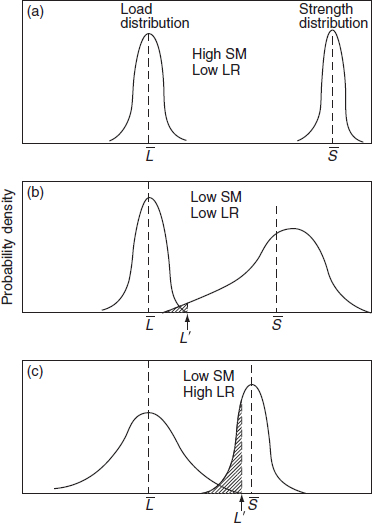
Figure 5.2 Effect of safety margin and loading roughness. Load L’ causes failure of a proportion of items indicated by the shaded area.

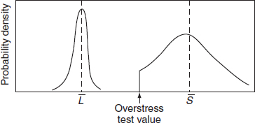
Figure 5.3 Truncation of strength distribution by screening.

Figure 5.2 (c) shows a low safety margin and high loading roughness due to a wide spread of the load distribution. This is a difficult situation from the reliability point of view, since an extreme stress event could cause a large proportion of the population to fail. Therefore, it is not economical to improve population reliability by screening out items likely to fail at these stresses. The options left are to increase the safety margin by increasing the mean strength, which might be expensive, or to devise means to curtail the load distribution. This is achieved in practice by devices such as current limiters and fuses in electronic circuits or pressure relief valves and dampers in pneumatic and hydraulic systems.

5.3 Analysis of Load–Strength Interference

The reliability of a part, for a discrete load application, is the probability that the strength exceeds the load:

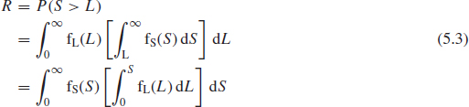
where f_S(S) is the pdf of strength and f_L(L) is the pdf of load.

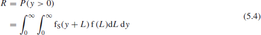
Also, if we define y = S – L, where y is a random variable such that

5.3.1 Normally Distributed Strength and Load

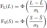
If we consider normally distributed strength and load, so that the cdfs are

if y = S − L, then = − and σ_y = ( + )^1/2. So

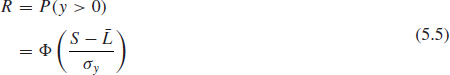
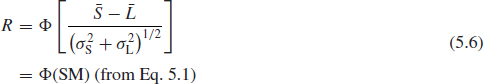
Therefore, the reliability can be determined by finding the value of the standard cumulative normal variate from the normal distribution tables or statistical calculators. The reliability can be expressed as

Example 5.1

A component has a strength which is normally distributed, with a mean value of 5000 N and a standard deviation of 400 N. The load it has to withstand is also normally distributed, with a mean value of 3500N and a standard deviation of 400 N. What is the reliability per load application?

The safety margin is

From Appendix 1,

5.3.2 Other Distributions of Load and Strength

The integrals for other distributions of load and strength can be derived in a similar way. For example, we may need to evaluate the reliability of an item whose strength is Weibull distributed, when subjected to loads that are extreme-value distributed. These integrals are somewhat complex and most of the time cannot be solved analytically. Therefore, Monte Carlo simulation, covered in Chapter 4, can be used to randomly select a sample from each distribution and compare them. After a sufficient number of runs, the probability of failure can be estimated from the results, which is demonstrated later in this chapter.

5.4 Effect of Safety Margin and Loading Roughness on Reliability (Multiple Load Applications)

For multiple load applications:

where n is the number of load applications.

Reliability now becomes a function of safety margin and loading roughness, and not just of safety margin. This complex integral cannot be reduced to a formula as Eq. (5.6), but can be evaluated using computerized numerical methods.

Figure 5.4 shows the effects of different values of safety margin and loading roughness on the failure probability per load application for large values of n, when both load and strength are normally distributed. The dotted line shows the single load application case (from Eq. 5.6). Note that the single load case is less reliable per load application than is the multiple load case.

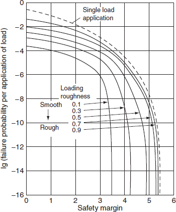
Figure 5.4 Failure probability–safety margin curves when both load and strength are normally distributed (for large n and n = 1) (Carter, 1997).

Since the load applications are independent, reliability over n load applications is given by

where p is the probability of failure per load application.

For small values of p the binomial approximation allows us to simplify this to

The reliability for multiple load applications can then be derived, if we know the number of applications, having used Figure 5.4 to derive the value of p. Once the safety margin exceeds a value of 3 to 5, depending upon the value of loading roughness, the failure probability becomes infinitesimal. The item can then be said to be intrinsically reliable. There is an intermediate region in which failure probability is very sensitive to changes in loading roughness or safety margin, whilst at low safety margins the failure probability is high. Figure 5.5 shows these characteristic regions. Similar curves can be derived for other distributions of load and strength. Figure 5.6 and Figure 5.7 show the failure probability – safety margin curves for smooth and rough loading situations for Weibull-distributed load and strength. These show that if the distributions are skewed so that there is considerable interference, high safety margins are necessary for high reliability. For example, Figure 5.6 shows that, even for a low loading roughness of 0.3, a safety margin of at least 5.5 is required to ensure intrinsic reliability, when we have a right-skewed load distribution and a left-skewed strength distribution. If the loading roughness is high (Figure 5.7), the safety margin required is 8. These curves illustrate the sensitivity of reliability to safety margin, loading roughness and the load and strength distributions.

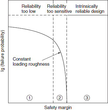
Figure 5.5 Characteristic regions of a typical failure probability–safety margin curve (Carter, 1997).

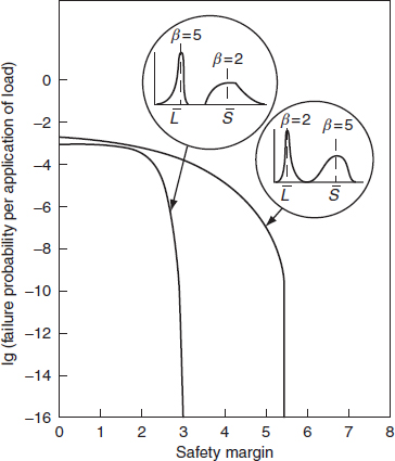
Figure 5.6 Failure probability–safety margin curves for asymmetric distributions (loading roughness = 0.3) (Carter, 1997).

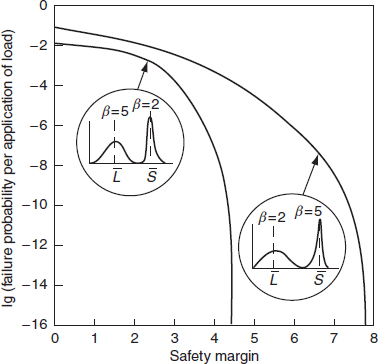
Figure 5.7 Failure probability–safety margin curves for asymmetric distributions (loading roughness = 0.9) (Carter, 1997).

Two examples of Load-Strength analysis application to design are given to illustrate the application to electronic and mechanical engineering.

Example 5.2 (electronic)

A design of a power amplifier uses a single transistor in the output. It is required to provide an intrinsically reliable design, but in order to reduce the number of component types in the system the choice of transistor types is limited. The amplifier must operate reliably at 50°C.

An analysis of the load demand on the amplifier based on customer usage gives the results in Figure 5.8. The mean ranking of the load test data is given in Table 5.1. A type 2N2904 transistor is selected. For this device the maximum rated power dissipation is 0.6 W at 25°C.

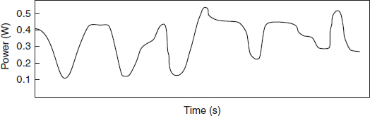
Figure 5.8 Load data (sampled at 10s intervals).

Table 5.1 Mean ranking of load test data.

Power (W)	Cumulative percentage time (cdf)
0.1	5%
0.2	25%
0.3	80%
0.4	98.5%
0.5	99.95%

The load test data shown in Table 5.1 can be analysed to find the best fitting distribution. There is a variety of commercial software packages with best fit capability including Weibull++¯ and @Risk¯ mentioned in the previous chapters. After applying the Weibull++ Distribution Wizard¯ program (see Chapter 3, Figure 3.17) we can see that the top three choices include Weibull, Normal and Gamma in that order. To simplify the calculations, let us select the normal, which has the parameters for the load distribution:

Alternatively, this could have been obtained by plotting the data from Table 5.1 on a normal distribution paper.

However, in this case we must consider the combined effects of power dissipation and elevated temperature. The temperature derating guidelines for the 2N2904 transistor advise 3.43 mW/K linear derating. Since we require the amplifier to operate at 50°C, the equivalent combined load distribution is normal, with the same SD, but with a mean which is (25 × 3.43) mW = 0.086 W higher. The mean load is now 0.238 + 0.086 = 0.324 W, with an unchanged standard deviation of 0.0783 W.

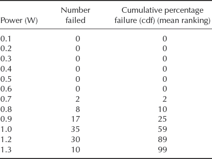
To derive the strength distribution, 100 transistors were tested at 25°C ambient, for 10 s at each power level (step stress), giving failure data as shown in Table 5.2. Similarly to the load in Table 5.1 these data are processed with Weibull++, indicating a normal distribution with mean power at failure (strength) of 0.9897 W and SD of 0.142 W.

Table 5.2 Failure data for 100 transistors.

Combining the load–strength data gives

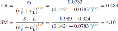
Therefore

This is the reliability per application of load for a single load application. Figure 5.4 shows that for multiple load applications (large n), the failure probability per load application (p) is about 10⁻¹¹(zone 2 of Figure 5.5). Over 10⁶ load applications the reliability would be about 0.999 99 (from Eq. 5.6).

In practice, in a case of this type the temperature and load derating guidelines described in Chapter 9 would normally be used. In fact, to use a transistor at very nearly its maximum temperature and load rating (in this case the measured highest load is 0.5 W at 25°C, equivalent to nearly 0.6 W at 50°C) is not good design practice, and derating factors of 0.5 to 0.8 are typical for transistor applications. The example illustrates the importance of adequate derating for a typical electronic component. The approach to this problem can also be criticised on the grounds that:

1. The failure (strength) data are sparse at the ‘weak’ end of the distribution. It is likely that batch-to-batch differences would be more important than the test data shown, and screening could be applied to eliminate weak devices from the population.
2. The extrapolation of the load distribution beyond the 0.5 W recorded peak level is dangerous, and this extrapolation would need to be tempered by engineering judgement and knowledge of the application.

Example 5.3 (mechanical fatigue)

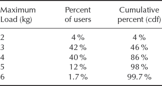
Customer usage data often come handy in obtaining the stress distribution of a load applied to the system. A washing machine manufacturer is trying to estimate the electric motor warranty cost due to fatigue failure for the first year of operation, which on average amounts to 100 cycles for the motor. The actual washing load sizes for the motors will vary depending on the way that the user runs each machine. In order to calculate warranty cost the manufacturer wants to estimate the percentage of returns that can be expected during the first year of operation. Even though the motor was designed to operate at the stresses exceeding the maximum allowable load of 6 kg, the life of the motor is clearly dependent on the applied load. That load varies based on customer usage patterns, so the question to be answered is which load size should be used in predicting the percentage of returns during warranty. At first step, the manufacturer decides to obtain the customer usage information by conducting a survey on a representative sample of customers and recording the sizes of the loads that they placed into their washing machines.

From this data set in Table 5.3 the distribution that gives the percentage of users operating washers at different loads can be determined. The cdf values in the third column can be processed similarly to the way it is done in Example 5.2. Using Weibull++ Distribution Wizard¯ (Section 3.7.1) it was determined that this data is best fitted with the lognormal distribution with μ = 1.12 and σ = 0.243.

Table 5.3 Maximum loads vs. percentages of the users applying those loads.

At the next step the manufacturer needs to obtain information on the life of the motor at different loads (or stress levels). Representative samples of the motor were tested to failure at five different loads. Then Weibull analysis (Section 3.4) was performed and the percentages of a population failing at 100 cycles at each load were determined and summarised in Table 5.4.

With the help of software the three parameter Weibull distribution was fitted to this data set and the following parameters were obtained: β = 1.69, η = 6.67, γ = 3.2.

Plotting two pdf functions in the same graph produces the diagram Figure 5.9 showing the overlapping area, where failures are expected to occur.

Now the last step is to calculate the area where the two distributions overlap. Since neither of the obtained distributions is normal (thus no closed form solution) the manufacturer decided to use Monte Carlo simulation to find the percentage of the cases where values from the load distribution exceed the value from the strength distribution. As mentioned in Chapter 4 there is a variety of commercial packages designed to run Monte Carlo simulations including the ‘Stress-Strength’ option imbedded in Weibull++¯. However, for simplicity the Excel spreadsheet solution similar to that in Chapter 4, Example 4.2 has been used. The lognormal load distribution can be simulated by the Excel¯ function = LOGINV(RAND(), 1.12, 0.243) (see Chapter 4, Table 4.1) and the 3-parameter Weibull Strength by = (6.67*(-LN(RAND()))^∧(1/1.69)) + 3.2. The manufacturer has conducted 10 000 simulation runs (Excel rows) and found that the number of rows where the load exceeded the strength was on average 1.2% of the total number of rows (10 000). Based on this analysis the manufacturer set aside the amount sufficient to cover 1.2% motor failures of the production volume during the warranty period.

Table 5.4 Washing machine loads vs.percent of motors failing at 100 cycles.

Maximum Load (kg)	Percent failed at 100 cycles (cdf)
4	2.73%
5	10.32%
6	20.6%
7	32.0%
9	54.6%

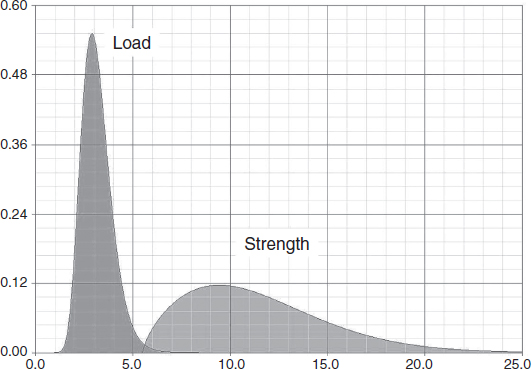
Figure 5.9 Load-Strength distribution chart generated with Weibull++¯ for Example 5.3 (Reproduced by permission of ReliaSoft).

5.5 Practical Aspects

The examples illustrate some of the advantages and limitations of the statistical engineering approach to design. The main difficulty is that, in attempting to take account of variability, we are introducing assumptions that might not be tenable, for example by extrapolating the load and strength data to the very low probability tails of the assumed population distributions. We must therefore use engineering knowledge to support the analysis, and use the statistical approach to cater for engineering uncertainty, or when we have good statistical data. For example, in many mechanical engineering applications good data exist or can be obtained on load distributions, such as wind loads on structures, gust loads on aircraft or the loads on automotive suspension components. We will call such loading situations ‘predictable’.

On the other hand, some loading situations are much more uncertain, particularly when they can vary markedly between applications. Electronic circuits subject to transient overload due to the use of faulty procedures or because of the failure of a protective system, or a motor bearing used in a hand power drill, represent cases in which the high extremes of the load distribution can be very uncertain. The distribution may be multimodal, with high loads showing peaks, for instance when there is resonance. We will call this loading situation ‘unpredictable’. Obviously it will not always be easy to make a definite classification; for example, we can make an unpredictable load distribution predictable if we can collect sufficient data. The methods described above are meaningful if applied in predictable loading situations. (Strength distributions are more often predictable, unless there is progressive strength reduction, which we will cover later.) However, if the loading is very unpredictable the probability estimates will be very uncertain. When loading is unpredictable we must revert to traditional methods. This does not mean that we cannot achieve high reliability in this way. However, evolving a reliable design is likely to be more expensive, since it is necessary either to deliberately overdesign or to improve the design in the light of experience. The traditional safety factors derived as a result of this experience ensure that a new design will be reliable, provided that the new application does not represent too far an extrapolation.

Moreover, the customer usage data utilized in both examples sometimes requires an additional layer of statistical treatment. Specifically, in Example 5.3 the manufacturer assumed the average of 100 motor cycles for the first year of operation. In reality, the number of cycles in the first year of motor operation should also be described by a statistical distribution due to differences in washing habits of the end users. This aspect of usage data will be discussed later in Chapter 7 covering variations in product usage and distribution environment.

Alternatively, instead of considering the distributions of load and strength, we can use discrete maximum/minimum values in appropriate cases. For example, we can use a simple lowest strength value if this can be assured by quality control. In the case of Example 5.2, we could have decided that in practice the transistors would not fail if the power is below 0.7 W, which would have given a safety factor of 1.4 above the 99.95% load cdf In other cases we might also assume that for practical purposes the load is curtailed, as in situations where the load is applied by a system with an upper limit of power, such as a hydraulic ram or a human operator. If the load and strength distributions are both curtailed, the traditional safety factor approach is adequate, provided that other constraints such as weight or cost do not make a higher risk design necessary.

The statistical engineering approach can lead to overdesign if it is applied without regard to real curtailment of the distributions. Conversely, traditional deterministic safety factor approaches can result in overdesign when weight or cost reduction must take priority.

In many cases, other design requirements (such as for stiffness) provide intrinsic reliability. The techniques described above should therefore be used when it is necessary to assess the risk of failure in marginal or critical applications.

As the examples in this chapter show, the ability to fit data into a distribution is important to a successful load-strength analysis. As mentioned before there is a variety of commercial software packages (Weibull++¯, @Risk¯, Minitab¯, Crystal Ball¯, etc.) with capability of finding the best fit distribution for sampled and/or cumulative percentage data.

In this chapter we have taken no account of the possibility of strength reduction with time or with cyclic loading. The methods described above are only relevant when we can ignore strength reduction, for instance if the item is to be operated well within the safe fatigue life or if no weakening is expected to occur. Reliability and life analysis in the presence of strength degradation is covered in Chapters 8 and 14.

Finally, it is important that reliability estimates that are made using these methods are treated only as very rough, order-of-magnitude figures.

Questions

1. Describe the nature of the load and strength distributions in four practical engineering situations (use sketches to show the shapes and locations of the distributions). Comment on each situation in relation to the predictability of failures and reliability, and in relation to the methods that can be used to reduce the probabilities of failure.
2. 1. Give the formulae for safety margin and loading roughness in situations where the load applied to an item and the strength of the item are assumed to be normally distributed.
   2. Sketch the relationship between failure probability and safety margin for different values of loading roughness, indicating approximate values for the parameters.
3. 1. If loads are applied randomly to randomly selected items, when both the loads and strengths are normally distributed, what is the expression for the reliability per load application?
   2. Describe and comment on the factors that influence the accuracy of reliability predictions made using this approach.
4. Describe two examples each from mechanical and electronic engineering by which extreme load and strength values are curtailed, in practical engineering design and manufacture.
5. If the tests described in Example 5.2 were repeated, and
   1. One transistor failed at 0.5 W, how would you re-interpret the results?
   2. The first 10 failures occurred at 0.8 W, how would you re-interpret the results?
6. Calculate the reliability (Eq. (5.3)) in the case where both random load and random strength are distributed exponentially. The pdfs are given by:

   

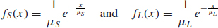
   where μ_L is the mean load and μ_S is the mean strength.

7. Electrolytic capacitor leads are designed to withstand a repetitive load applied to a circuit board mounted on a moving platform. The lead's yield stress is normally distributed with the mean of 100 MPa and the standard deviation of 20 MPa. The stress generated as a result of the repetitive load during the capacitor's life time is also normally distributed with the mean of 60 MPa and the standard deviation of 15 MPa:
   1. Calculate the safety margin, SM.
   2. Calculate the loading roughness, LR.
   3. Calculate the expected reliability of the capacitor.
8. A connecting rod must transmit a tension load which trials show to be lognormally distributed, with the following parameters: μ = 9.2 and σ = 1.1. Tests on the material to be used show a lognormal strength distribution as follows: μ = 11.8 and σ = 1.3. A large number of components are to be manufactured, so it is not feasible to test each one. Calculate the expected reliability of the component using Monte Carlo simulation.

Bibliography

Carter, A. (1997) Mechanical Reliability and Design, Wiley.

Kapur K. and Lamberson L. (1977) Reliability in Engineering Design, Wiley.

Palisade Corporation (2005) Guide to Using @Risk. Advanced Risk Analysis for Spreadsheets’ Palisade Corporation. Newfield, New York. Available at http://www.palisade.com.

ReliaSoft (2002) Prediction Warranty Returns Based on Customer Usage Data. Reliability Edge, Quarter 1: Volume 3, Issue 1. Available at http://www.reliasoft.com/newsletter/1q2002/usage.htm (Accessed 22 March 2011).

ReliaSoft (2008) Weibull++¯ User's Guide, ReliaSoft Publishing.

Wasserman, G. (2003) Reliability Verification, Testing and Analysis in Engineering Design, Marcel Dekker.