14

Reliability Demonstration and Growth

14.1 Introduction

As described in Chapter 12, reliability testing is the cornerstone of a reliability engineering programme. Chapter 12 emphasized the importance of reliability testing being planned primarily to improve reliability by showing up potential weaknesses. However, a properly designed series of tests can also generate data that would be useful in determining if the product meets specified requirements to operate without failure during its mission life, or to achieve a specified level of reliability. Many product development programmes require a series of environmental tests to be completed to demonstrate that the reliability requirements are met by the manufacturer and then demonstrated to the customer.

Reliability demonstration testing is usually performed at the stage where hardware (and software when applicable) is available for test and is either fully functional or can perform all or most of the intended product functions. While it is desirable to be able to test a large population of units to failure in order to obtain information on a product's or design's reliability, time and resource constraints sometimes make this impossible. In cases such as these, a test can be run on a specified number of units, or for a specified amount of time, that will demonstrate that the product has met or exceeded a given reliability at a given confidence level. In the final analysis, the actual reliability of the units will of course remain unknown, but the reliability engineer will be able to state that certain specifications have been met. This chapter will discuss those requirements and different ways of achieving them in the industrial setting.

14.2 Reliability Metrics

Most product design specifications come with some form of reliability requirements, which are expressed as reliability metrics. If the system is complex those requirements may come from reliability apportionment activities (Chapter 6) or other requirements generated at the system, subsystem or component level.

Probably the most common reliability metric is the simple reliability function R(t). For example a product specification may state that the expected reliability over a 5-yr life should be no less than 98.0% meaning R(5 yrs) = 0.98. A reliability requirement often comes with a specified confidence level based on a test sample size. This will be covered in the next section.

Another popular metric is mean time between failures (MTBF) (Section 2.6.3). MTBF is a characteristic of a repairable system with constant failure rate (see the exponential distribution Eq. (2.27)). MTBF is often misinterpreted by non-reliability engineers as an average time between consecutive failures in all of the product population even though those could be failures of different units. Therefore it is recommended to use other reliability demonstration metrics whenever possible. For non-repairable systems with constant failure rate mean time to failure (MTTF) is used in place of MTBF (see Chapters 1 and 2). Consequently, the failure rate λ can also be used as a reliability metric for both repairable and non repairable systems.

B_X-life (Section 3.4.5) is another common reliability metric, which is often used as B₁₀ specification, the product life at which 10% of the population is expected to fail (i.e. 90% reliability).

PPM (parts per million) can also be used as a reliability metric, although it is more often used to measure manufacturing quality in production. In the case of reliability, PPM would be a function of time, which would represent the number of parts per million failed during the time interval [0; t], therefore:

One form of reliability metric can often be converted to the other and used interchangeably.

Example 14.1

The initial product requirement defines B₁₀ life of 5 years. Convert this requirement to other reliability metrics. Under the assumption of exponentially distributed failures:

Solving (14.2) we obtain MTTF = 47.5 years. Failure rate λ = 1/MTTF = 0.021 failures per year or assuming 24 hours per day operation λ = 0.0210/(365 × 24) = 2.4 × 10⁻⁶ failures per hour. Also, based on (14.1) R(5yrs) = 0.9 would mean 100 000 PPM at 5 yrs.

14.3 Test to Success (Success Run Method)

Test to success, where failures are undesirable has been covered in Chapter 12. Industry dependent, it is also referred as success run testing, attribute test, zero failure substantiation test or mission life test. Under those conditions a product is subject to a test, often accelerated representing an equivalent to one field life (test to a bogey), which is expected to be completed without failure by all the units in the test sample. Methods of estimating the test equivalent of one field or mission life were discussed in Section 13.6.

14.3.1 Binomial Distribution Approach

Success run test statistics are most often based on the binomial distribution presented in Section 2.10.1. The binomial pdf is described by Chapter 2 Eq. (2.37) which can be applied to the test situations with only two possible outcomes: pass or fail. Therefore, assuming that reliability R = p in (2.37) the probability of a product to survive (based on the binomial cdf) can be presented in the form of:

where: R = unknown reliability.

Table 14.1 Required test sample sizes for reliability demonstration at 50 and 90% confidence.

If k = 0 (no failures) (14.3) turns into a simple equation for success run testing:

(14.4) can be solved for the test sample size N as:

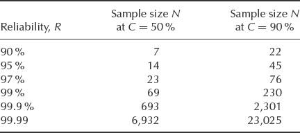
When demonstrated reliability R approaches 1.0 the required sample size N based on Eq. (14.5) approaches infinity. Table 14.1 shows the required test sample sizes for statistical confidence of 50 and 90% based on (14.5).

Product design and validation requirements often explicitly specify reliability and confidence level for their reliability demonstration programmes. For example, a common requirement in the automotive industry is to demonstrate reliability of 97.0% with 50% confidence. According to Table 14.1 this would require 23 units to be tested without failure to an equivalent of one field life.

14.3.2 Success Run Test with Undesirable Failures

When undesirable failures occur during test to success, reliability can still be estimated using Eq. (14.3). However (14.3) can be difficult to solve for R, especially when k > 2, therefore an approximation chi-square formula can be used instead:

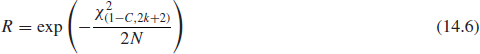
The derivation of (14.6) is based on the estimates for the MTBF confidence intervals covered later in Section 14.6. χ² values can be found in Appendix 2 or calculated using the Excel function CHIINV(1-C, 2k + 2).

14.4 Test to Failure Method

Testing to demonstrate reliability when failures occur during test can be analysed using the life data analysis methods described in detail in Chapter 3. Based on results of life data analysis we can model the reliability function R(t) based on the chosen distribution and generate confidence bounds (Section 3.6) corresponding to the confidence level required for the demonstrated reliability. The two or three-parameter Weibull distribution (Section 3.4) is probably the most common choice for reliability practitioners to model the R(t) function. The value of the Weibull slope β also gives insight into the product's bathtub curve (infant mortality, useful life, or wearout mode).

The downside of the test to failure method is longer test times compared to equivalent success run tests. Whereas success run testing requires test durations equivalent to one product field life (or its accelerated equivalent), a test to failure requires at least twice that in order to allow time to generate enough failures for the life data analysis. Additionally, test to failure requires some form of monitoring equipment to record failure times. Therefore, due to ever-increasing pressure to reduce development cycles, project managers often opt for success run testing instead of testing to failure.

14.5 Extended Life Test

Cost consideration is always an important part of a test planning process. Test sample size carries the cost of producing each test sample (which can be quite high in some industries), equipping each sample with monitoring equipment and providing an adequate test capacity to accommodate all the required samples. A large sample may also require additional floor space for additional test equipment, such as temperature/humidity chambers or vibration shakers, which can be quite costly.

Test duration can be used as a factor to reduce the cost of reliability demonstration. In the cases where test samples are expensive it may be advantageous to test fewer units, though for longer periods of time.

14.5.1 Parametric Binomial Method

Combining the success run formulae (14.4) with 2-parameter Weibull reliability, Eq. (2.31) Lipson and Sheth (1973) developed the relationship between two test sets with (N₁, t₁) and (N₂, t₂) characteristics needed to demonstrate the same reliability and confidence level.

where: β = Weibull slope for primary failure mode (known or assumed).

Therefore it is possible to extend test duration in order to reduce test sample size. Therefore if t₁ is equivalent to one mission life t₂ = Lt₁, where L is the life test ratio. Thus combining this with (14.7).

With the use of (14.8) the success run formula (14.4) will transform into:

Relationship (14.9) is often referred as the parametric binomial model. Test sample size reduction at the expense of longer testing can also be beneficial in the cases with limited test capacities. For example, if an environmental chamber can accommodate only 18 test samples, while 23 are required for the reliability demonstration, test time can be extended to demonstrate the same reliability with only 18 units.

The required number of test samples can be reduced L^β times in the cases of extended life testing (L > 1).

Therefore this approach allows additional flexibility to minimize the cost of testing by adjusting test sample size up or down to match the equipment capacity.

Example 14.2

The design specification requirement is 97.0% reliability with 50% confidence for the 1000 hours temperature test corresponding to one product field life. A temperature chamber equipped with a test monitoring rack has a capacity of only 15 units. Calculate the test time required to meet the above reliability requirement, assuming the Weibull slope β = 2.0.

According to (14.5) and Table 14.1 the sample size of 23 would be required to demonstrate 97% reliability with 50% confidence. Thus solving (14.9) for L and substituting R = 97.0%, C = 50%, N = 15, and β = 2.0 produces:

Therefore the original test duration of 1000 hours should be extended to Lt = 1.232 × 1000 = 1232 hours without failure in order to demonstrate the required reliability with 15 samples instead of 23 (see also Figure 14.2).

14.5.2 Limitations of the Parametric Binomial Model

This method has been successfully applied to both extended and reduced life testing. However it is not recommended to change the test to a bogey time by more than ±50%, because it may violate the assumptions of the parametric binomial model. Since (14.9) uses Weibull slope β it assumes a particular trend in the hazard rate. For example if β = 3.0 the model reflects the wear-out rate corresponding to the Weibull slope of 3.0. Significantly extending test time may accelerate the wear out process where β > 3.0, thus increasing the probability of failure beyond the model's assumptions. The reverse is also true. Shortening test time may shift the failure pattern from the wear-out phase on the bathtub curve to the useful life. That would effectively reduce the β -value to 1.0, again violating the assumptions of the parametric binomial model.

14.6 Continuous Testing

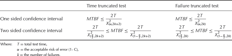
During continuous testing, the mean time between failures can be calculated as the total test time T amongst all tested units divided by the number of failures k (MTBF = T/k). When a product's failure rate is considered constant, the χ² distribution may be used to calculate confidence intervals around MTBF, and therefore demonstrated reliability.

The lower and upper confidence limits for data which are generated by a homogeneous Poisson process are given in Table 14.2. It shows the one-sided and two-sided limits for the conditions where the test is stopped at the kth failure, that is a failure truncated test, and for a time truncated test, (i.e. test is stopped after a predetermined time). Values of χ² for different risk factors α and degrees of freedom are given in Appendix 2 or can be calculated using Excel statistical function CHIINV.

In the case of non-repairable systems MTBF becomes MTTF.

Table 14.2 MTBF confidence limits.

Example 14.3

Ten units were tested for a total of 2000 h and 3 failures occurred. The test was time-truncated. Assuming a CFR, what is the demonstrated 90% lower confidence limit on reliability at 100 operating hours?

Using the appropriate equation from Table 14.2 and the Excel function CHIINV (or Appendix 2):

Therefore, based on the exponential distribution:

14.7 Degradation Analysis

Product testing takes time and it may take too long for the product to fail operating under normal or even accelerated stress conditions. Test to success may also take a prohibitively long time when simulating long field lives (e.g. 15–30 years). Degradation analysis introduced in Chapter 7 is one way of demonstrating reliability within a relatively short period of time. Many failure mechanisms can be directly linked to the degradation of part of the product, and degradation analysis allows the user to extrapolate to a failure time based on the measurements of degradation or change in performance over time. Examples of product degradation include the wear of brake pads, crack propagation due to material fatigue, decrease in conductivity, loss of product performance such as generated power, and so on.

For effective degradation analysis it is necessary to be able to define a level of degradation or performance which constitutes a failure. Once this failure threshold is established it is a relatively simple matter to use basic mathematical models to extrapolate the performance measurements over time to the point where the failure is expected to occur. Once the extrapolated failure times have been determined, it is a matter of conducting life data analysis to model and analyse the demonstrated reliability of the tested items.

Figure 14.1 demonstrates the concept of degradation analysis, where the measurements were taken at 0, 250 and 500 hours. This data was then extrapolated to estimate the point in time where the degradation parameter crosses the ‘failure threshold’ and becomes a failure. Most commonly used extrapolation models include linear (y = bx+c), exponential (y = be^axe) and power (y = bx^a). Other models are also available in commercial data analysis software packages (see ReliaSoft, 2006).

Figure 14.1 Degradation analysis diagram.

Before conducting reliability demonstration based on degradation analysis the following should be considered:

• The chosen degradation parameter has to be critical to the product failure and represent the dominant failure mechanism.
• Verify that the chosen parameter is affected by the test. This parameter may in reality degrade due to other causes, such as poor quality or be unrelated to the test altogether.
• The chosen parameter should exhibit a clear degradation trend. It would invalidate the test if the product exhibits fluctuations in the parameter value over time.
• As with any sort of extrapolation, one must be careful not to extrapolate too far beyond the actual range of data in order to avoid large inaccuracies.

Simple degradation analysis can be done with an Excel spreadsheet by extrapolating data points and estimating the time when the degradation value reaches the threshold. However it is always more efficient to use software specifically designed for that purpose.

14.8 Combining Results Using Bayesian Statistics

It can be argued that the result of a reliability demonstration test is not the only information available on a product, but that information is available prior to the start of the test, from component and subassembly tests, previous tests on the product and even intuition based upon experience. Why should this information not be used to supplement the formal test result? Bayes theorem (Chapter 2) states (Eq. 2.9):

enabling us to combine such probabilities. Eq. (2.9) can be extended to cover probability distributions:

where λ is a continuous variable and φ represents the new observed data: p(λ) is the prior distribution of λ; p(λ|φ) is the posterior distribution of λ, given φ; and f (φ|λ) is the sampling distribution of φ, given λ.

Let λ denote failure rate and t denote successful test time. Let the density function for λ be gamma distributed with

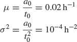
If the prior parameters are a₀, t₀, then the prior mean failure rate is μ = a₀/t₀ and the prior variance is σ² = a₀/ (appropriate symbol changes in Eq. 2.28). The posterior will also be gamma distributed with parameters a₁ and t₁ where a₁ = a₀ + n and t₁ = t₀ + t and n is the number of events in the interval from 0 to t. The confidence limits on the posterior mean are /2t₁.

Example 14.4

The prior estimate of the failure rate of an item is 0.02, with a standard deviation of 0.01. A reliability demonstration test results in n = 14 failures in t = 500 h. What is the posterior estimate of failure rate and the 90% lower confidence limit?

The prior mean failure rate is

Therefore,

The posterior estimate for failure rate is

This compares with the traditional estimate of the failure rate from the test result of 14/500 = 0.028 h⁻¹.

The 90% lower confidence limit on the mean is

compared with the traditional estimate (from Table 14.2) of

In Example 14.4 use of the prior information has resulted in a failure rate estimate lower than that given by the test, and closer confidence limits.

The Bayesian approach is somewhat controversial in reliability engineering, particularly as it can provide a justification for less reliability testing. For example, Kleyner et al. (1997) proposed a method to reduce sample size required for a success run test in order to demonstrate target reliability with a specified confidence. Choosing a prior distribution based on subjective judgement, expert opinion, or other test or field experience can also be contentious. Combining subassembly test results in this way also ignores the possibility of interface problems.

Another downside of the method is that an unfavourable prior can actually have the opposite effect on reliability demonstration, that is increase the required test time or sample size. The Bayesian approach is not normally part of a product validation program; however there have been efforts to incorporate it in reliability standards. For example Yates (2008) describes the work on an Australian defense standard for Bayesian reliability demonstration.

14.9 Non-Parametric Methods

Non-parametric statistical techniques (Section 2.13) can be applied to reliability measurement. They are arithmetically very simple and so can be useful as quick tests in advance of more detailed analysis, particularly when no assumption is made of the underlying failure distribution.

14.9.1 The C-Rank Method

If n items are tested and k fail, the reliability of the sample is

where C denotes the confidence level required, using the appropriate rank (for median ranks see Chapter 3, Eq. (3.5) and Appendix 4 for 5% and 95% ranks).

Example 14.5

Twenty items were subjected to a 100 h test in which three failed. What is the reliability at the 50% and 95% lower confidence levels?

From Eq. (3.5) and Appendix 4, the median and 95% rank tables, the C-rank of four items in a sample of 21 is:

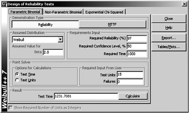
Figure 14.2 Solution to Example 14.2 using Weibull++¯ reliability demonstration calculator DRT (reproduced by permission of ReliaSoft).

14.10 Reliability Demonstration Software

Various software packages are available to conduct quick reliability demonstration calculations according to the methods covered above. For example, Weibull++¯ has a built-in calculator called DRT (Design of Reliability Tests) allowing the user to expeditiously estimate the required test durations, sample sizes, confidence limits, and so on based on the available information. Figure 14.2 shows the solution to Example 14.2 using the DRT option. It calculates the extended test time using the parametric binomial model. Some of those calculation features are available in Minitab¯, CARE¯ by BQR, WinSMITH¯, Reliass¯ and others.

14.11 Practical Aspects of Reliability Demonstration

In the industrial setting involving suppliers and customers, test and validation programmes including reliability demonstration often require customer approvals, which sometimes become a source of contention. In some instances the customer may set the reliability targets to a level which is not easy to demonstrate by a reasonable amount of testing.

It is important to remember that demonstrating high reliability is severely limited by the test sample size required (see Table 14.1) no matter which method is chosen and therefore by the amount of money available to spend on testing activities. Moreover, the issue of reliability demonstration gets even more confused when the customer directly links it with reliability prediction (see Kleyner and Boyle (2004) on reliability demonstration vs. reliability prediction). As mentioned in Chapter 6 most reliability prediction methods are based on generic component failure rates and therefore can generate values that have large uncertainty. Also, there is often uncertainty with regard to demonstrated reliability. Therefore discrepancies between the two can be expected. In order to clarify some of those issues, following are the arguments against attempting to demonstrate high reliability by testing a statistically significant number of units.

Firstly, for example a reliability demonstration of R = 99.9% implies 0.1% accuracy, which cannot possibly be obtained economically or practically with the methods described. Most of the tests performed by reliability engineers are accelerated tests with all the uncertainties associated with testing under conditions different from those in the field, the greatest contributor to which would be the field to test correlation. In other words, based on a test lasting from several hours to several weeks, we are trying to draw conclusions about the behaviour of the product in the field for the next 10–15 years. With so many unknown factors the overall uncertainty well exceeds 0.1% .

Secondly, system interaction problems contribute heavily to warranty claims. The analysis of warranties (Chapter 13, Figure 13.9) shows that reliability related problems comprise only part of the field problems, thus even if such a high reliability is demonstrated, it would not nearly guarantee that kind of performance in the field, since many other failure factors would be present.

Thirdly, calculations involving reliability demonstration are usually based on lower confidence bounds, therefore by demonstrating 95% reliability at a lower confidence bound we are in fact demonstrating R ≥ 0.95. Therefore the actual field reliability will most likely be higher than the demonstrated number. Demonstration testing of more units will not generally make the product more reliable, but designing for reliability will.

Fourthly, test requirements are often developed based on stresses corresponding to environmental conditions and user profiles well above average severity (see Section 7.3.2.1). Therefore the demonstrated reliability will be much higher when test results are applied to the population of users from all segments of the usage distribution.

And lastly, when very high reliability is specified (e.g. R > 0.999 in safety-related applications), reliability demonstration by test may be totally impracticable. Due to the test sample size limitations, analysis methods such as reliability modelling and simulation, finite element analysis, FMECA and others should be emphasized.

All of these points are reasons why quantitative reliability demonstrations should be used with care. It is essential that possible points of contention, such as definitions of failures, what can and cannot be demonstrated by test, and others, are agreed in advance.

14.12 Standard Methods for Repairable Equipment

This section describes standard methods of test and analysis which are used to demonstrate compliance with reliability requirements.

The standard methods are not substitutes for the statistical analysis methods described earlier in this chapter. They may be referenced in procurement contracts, particularly for government equipment, but they may not provide the statistical engineering insights given, for example, by life data analysis. Therefore the standards should be seen as complementary to the statistical engineering methods and useful (or mandatory) for demonstrating and monitoring reliability of products which are into or past the development phase.

14.12.1 Probability Ratio Sequential Test (PRST) (US MIL-HDBK-781)

The best known standard method for formal reliability demonstration testing for repairable equipment which operates for periods of time, such as electronic equipment, motors, and so on, is US MIL-HDBK-781: Reliability Testing for Engineering Development, Qualification and Production (see Bibliography). It provides details of test methods and environments, as well as reliability growth monitoring methods (see Section 14.13).

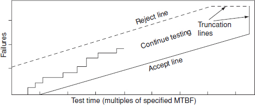
Figure 14.3 Typical probability ratio sequential test (PRST) plan.

MIL HDBK-781 testing is based on probability ratio sequential testing (PRST), the results of which (failures and test time) are plotted as in Figure 14.3. Testing continues until the ‘staircase’ plot of failures versus time crosses a decision line. The reject line (dotted) indicates the boundary beyond which the equipment will have failed to meet the test criteria. Crossing the accept line denotes that the test criteria have been met. The decision lines are truncated to provide a reasonable maximum test time. Test time is stated as multiples of the specified MTBF. British and international standards for reliability demonstration are based on MIL-HDBK-781 (see Bibliography).

14.12.2 Test Plans

MIL-HDBK-781 contains a number of test plans, which allow a choice to be made between the statistical risks involved (i.e. the risk of rejecting an equipment with true reliability higher than specified or of accepting an equipment with true reliability lower than specified) and the ratio of minimum acceptable to target reliability. The risk of a good equipment (or batch) being rejected is called the producer's risk and is denoted by α. The risk of a bad equipment (or batch) being accepted is called the consumer's risk, denoted by β. MIL-HDBK-781 test plans are based upon the assumption of a constant failure rate, so MTBF is used as the reliability index. Therefore MIL-HDBK-781 tests are appropriate for equipment where a constant failure rate is likely to be encountered, such as fairly complex maintained electronic equipment, after an initial burn-in period. Such equipment in fact was the original justification for the development of the precursor to MIL-HDBK-781, the AGREE report (Section 1.8). If predominating failure modes do not occur at a constant rate, tests based on the methods described in Chapter 2 should be used. In any case it is a good idea to test the failure data for trend, as described in Section 2.15.1.

The criteria used in MIL-HDBK-781 are:

1. Upper test MTBF, θ₀. This is the MTBF level considered ‘acceptable’.
2. Lower test MTBF, θ₁. This is the specified, or contractually agreed, minimum MTBF to be demonstrated.
3. Design ratio, d = θ₀/θ₁.
4. Producer's risk, α (the probability that equipment with MTBF higher than θ₁ will be rejected).
5. Consumer's risk β (the probability that equipment with MTBF lower than θ₀ will be accepted).

Table 14.3 MIL-HDBK-781 PRST plans.

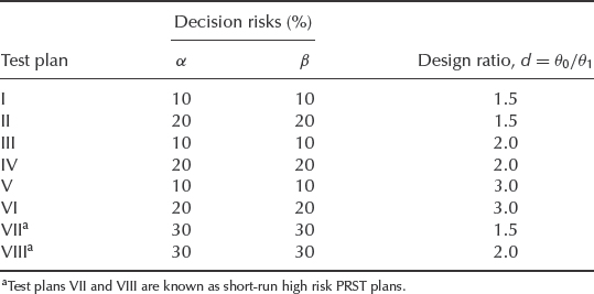
The PRST plans available in MIL-HDBK-781 are shown in Table 14.3. In addition, a number of fixed-length test plans are included (plans IX–XVI), in which testing is required to be continued for a fixed multiple of design MTBF. These are listed in Table 14.4. A further test plan (XVII) is provided, for production reliability acceptance testing (PRAT), when all production items are to be tested. The plan is based on test plan III. The test time is not truncated by a multiple of MTBF but depends upon the number of equipments produced.

14.12.3 Statistical Basis for PRST Plans

PRST is based on the statistical principles described in Section 14.6 and the assumption of a constant failure rate. The decision risks are based upon the risks that the estimated MTBF will not be more than the upper test MTBF (for rejection), or not less than the lower test MTBF (for acceptance).

We thus set up two null hypotheses:

Table 14.4 MIL-HDBK-781 fixed length test plans.

The probability of accepting H₀ is (1 − α), if = θ₁; the probability of accepting H₁ is β, if = θ₀. The time at which the i^th failure occurs is given by the exponential distribution function f (t_i) = (1/θ) exp(−t_i/θ). The sequential probability ratio, or ratio of the expected number of failures given θ = θ₀ or θ₁, is

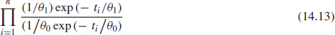
where n is the number of failures.

The upper and lower boundaries of any sequential test plan specified in terms of θ₀, θ₁, α and β can be derived from the sequential probability ratio. However, arbitrary truncation rules are set in MIL-HDBK-781 to ensure that test decisions will be made in a reasonable time. The truncation alters the accept and reject probabilities somewhat compared with the values for a non-truncated test, and the α and β rules given in MIL-HDBK-781 are therefore approximations. The exact values can be determined from the operating characteristic (OC) curve appropriate to the test plan and are given in MIL-HDBK-781. The OC curves are described in the next section.

14.12.4 Operating Characteristic Curves and Expected Test Time Curves

An operating characteristic (OC) curve can be derived for any sequential test plan to show the probability of acceptance (or rejection) for different values of true MTBF. Similarly, the expected test time (ETT – time to reach an accept or reject decision) for any value of θ can be derived. OC and ETT curves are given in MIL-HDBK-781 for the specified test plans. Typical curves are shown in Figure 14.4 and Figure 14.5.

14.12.5 Selection of Test Criteria

Selection of which test plans to use depends upon the degrees of risk which are acceptable and upon the cost of testing. For example, during development of new equipment, when the MTBF likely to be achieved might be uncertain, a test plan with 20% risks may be selected. Later testing, such as production batch acceptance testing, may use 10% risks. A higher design ratio would also be appropriate for early development reliability testing. The higher the risks (i.e. the higher the values of α and β) and the lower the design ratio, the longer will be the expected test duration and therefore the expected cost.

Figure 14.4 Operating characteristic (OC) curve. Test plan 1: α = 10%, β = 10% and d = 1.5.

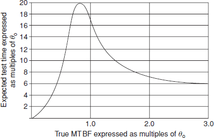
Figure 14.5 Expected test time (ETT) curve. Test plan 1: α = 10%, β = 10% and d = 1.5.

The design MTBF should be based upon reliability prediction, development testing and previous experience. MIL-HDBK-781 requires that a reliability prediction be performed at an early stage in the development programme and updated as development proceeds. We discussed the uncertainties of reliability prediction in Chapter 6. However, this should only apply to the first reliability test, since the results of this can be used for setting criteria for subsequent tests.

The lower test MTBF may be a figure specified in a contract, as is often the case with military equipment, or it may be an internally generated target, based upon past experience or an assessment of market requirements.

14.12.6 Test Sample Size

MIL-HDBK-781 provides recommended sample sizes for reliability testing. For a normal development programme, early reliability testing (qualification testing) should be carried out on at least two equipments. For production reliability acceptance testing the sample size should be based upon the production rate, the complexity of the equipment to be tested and the cost of testing. Normally at least three equipments per production lot should be tested.

14.12.7 Burn-In

If equipment is burned-in prior to being submitted to a production reliability acceptance test, MIL-HDBK-781 requires that all production equipments are given the same burn-in prior to delivery.

14.12.8 Practical Problems of PRST

Reliability demonstration testing using PRST is subject to severe practical problems and limitations, which cause it to be a controversial method. We have already covered one fundamental limitation: the assumption of a constant failure rate. However, it is also based upon the implication that MTBF is an inherent parameter of a system which can be experimentally demonstrated, albeit within confidence limits. In fact, reliability measurement is subject to the same fundamental constraint as reliability prediction: reliability is not an inherent physical property of a system, as is mass or electric current. The mass or power consumption of a system is measurable (also within statistical bounds, if necessary). Anyone could repeat the measurement with any copy of the system and would expect to measure the same values. However, if we measure the MTBF of a system in one test, it is unlikely that another test will demonstrate the same MTBF, quite apart from considerations of purely statistical variability. In fact there is no logical or physical reason to expect repeatability of such experiments. This can be illustrated by an example.

Suppose a system is subjected to a PRST reliability demonstration. Four systems are tested for 400 hours and show failure patterns as follows:

No. 1	2 memory device failures (20 h, 48 h)
	1 connector intermittent (150 h)
	1 capacitor short circuit (60 h)
No. 2	1 open-circuit PCB track (40 h)
	1 IC socket failure (200 h)
No. 3	No failures
No. 4	1 shorted connector (trapped on assembly) (0 h)
Total failures: 6
Total running time: 1600 h.
Observed MTBF = 267 h

Note that these failures are quite typical. However, if the experiment were repeated with another four systems, there would be no reason to expect the same number or pattern of failures. If the same four systems were tested for another 1600 hours the pattern of failures would almost certainly be different. The pattern of failures and their likelihood can be influenced by quality control of manufacture and repair. Therefore the MTBF measured in this test is really no more than historical data, related to those four systems over that period of their lives. It does not predict the MTBF of other systems or of those four over a subsequent period, any more than four sales in one day would be a prediction of the next day's sales. If any design or process changes are made as a result of the test, forecasting becomes even more uncertain.

Of course, if a large number of systems were tested we would be able to extrapolate the results with rather greater credibility and to monitor trends (e.g. average failures per system). However, PRST can seldom be extended to such large quantities because of the costs involved.

PRST is often criticized on the grounds that in-service experience of MTBF is very different to the demonstrated figure. From the discussion above this should not surprise anyone. In addition, in-service conditions are almost always very different to the environments of MIL-HDBK-781 testing, despite attempts to simulate realistic conditions in CERT.

PRST is not consistent with the reliability test philosophy described in Chapter 12, since the objective is to count failures and to hope that few occur. An effective reliability test programme should aim at generating failures, since they provide information on how to improve the product. Failure-counting should be a secondary consideration to failure analysis and corrective action. Also, a reliability test should not be terminated solely because more than a predetermined number of failures occur. PRST is very expensive, and the benefit to the product in terms of improved reliability is sometimes questionable.

14.12.9 Reliability Demonstration for One-Shot Items

For equipment which operate only once, or cyclically, such as pyrotechnic devices, missiles, fire warning systems and switchgear, the sequential method of testing based on operating time may be inappropriate. Statistical acceptance sampling methods can be used for such items, as described in Chapter 15. Alternatively, a MIL-HDBK-781 test could be adapted for items which operate cyclically, using a baseline of mean cycles to failure, or MTBF assuming a given cycling rate.

14.13 Reliability Growth Monitoring

14.13.1 The Duane Method

It is common for new products to be less reliable during early development than later in the programme, when improvements have been incorporated as a result of failures observed and corrected. Similarly, products in service often display reliability growth. This was first analysed by J. T. Duane, who derived an empirical relationship based upon observation of the MTBF improvement of a range of items used on aircraft. Duane observed that the cumulative MTBF θ_c(total time divided by total failures) plotted against total time on log–log paper gave a straight line. The slope (α) gave an indication of reliability (MTBF) growth, that is

where θ₀ is the cumulative MTBF at the start of the monitoring period T₀. Therefore,

The relationship is shown plotted in Figure 14.6.

The slope α gives an indication of the rate of MTBF growth and hence the effectiveness of the reliability programme in correcting failure modes. Duane observed that typically α ranged between 0.2 and 0.4, and that the value was correlated with the intensity of the effort on reliability improvement.

The Duane method is applicable to a population with a number of failure modes which are progressively corrected, and in which a number of items contribute different running times to the total time. Therefore it is not appropriate for monitoring early development testing, and it is common for early test results to show a poor fit to the Duane model. The method is also not consistent with the use of accelerated tests during development, since the objective of these is to force failures, not to generate reliability statistics, as described in Chapter 12.

Figure 14.6 Duane reliability growth.

We can derive the instantaneous MTBF θ_i of the population by differentiation of Eq. (14.14)

where k is the number of failures. Therefore,

(/θ₀) is a constant. Differentiation gives

So

θ_i is shown in Figure 14.6. The plot of θ_i is parallel to that for θ_c. A reliability monitoring programme may be directed towards a target either for cumulative or instantaneous MTBF.

After the end of a development programme in which MTBF growth is being managed, the anticipated MTBF of production items is θ_i, measured at the end of the programme. This assumes that the development testing accurately simulated the expected in-use stresses of the production items and that the standard of items being tested at the end of the development programme fully represents production items. Of course, these assumptions are often not valid and extrapolations of reliability values from one set of conditions to another must always be considered to be tentative approximations. Nevertheless, the empirical Duane method provides a reasonable approach to monitoring and planning MTBF growth for complex systems.

The Duane method can also be used in principle to assess the amount of test time required to attain a target MTBF. If the MTBF is known at some early stage, the test time required can be estimated if a value is assumed for α. The value chosen must be related to the expected effectiveness of the programme in detecting and correcting causes of failure. Knowledge of the effectiveness of past reliability improvement programmes operated by the organization can provide guidance in selecting a value for α. The following may be used as a guide:

• α = 0.4 − 0.6. Programme dedicated to the elimination of failure modes as a top priority. Use of accelerated (overstress) tests. Immediate analysis and effective corrective action for all failures.
• α = 0.3 − 0.4. Priority attention to reliability improvement. Normal (typical expected stresses) environment test. Well-managed analysis and corrective action for important failure modes.
• α = 0.2. Routine attention to reliability improvement. Testing without applied environmental stress. Corrective action taken for important failure modes.
• α = 0.2–0. No priority given to reliability improvement. Failure data not analysed. Corrective action taken for important failure modes, but with low priority.

Example 14.6

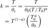
The first reliability qualification test on a new electronic test equipment generates 11 failures in 600 h, with no one type of failure predominating. The requirement set for the production standard equipment is an MTBF of not less than 500 h in service. How much more testing should be planned, assuming values for α of 0.3 and 0.5?

When θ_i = 500,

Using θ₀ = 54.4, from Eq. (14.14),

Graphical construction can be used to derive the same result, as shown in Figure 14.7 [tan⁻¹(0.3) = 17° tan⁻¹(0.5) = 27° θ_i = θ_c/(1 − α)].

Obviously nearly 300 000 h of testing is unrealistic, and therefore in this case a value for α of 0.5 would have to be the objective to achieve the MTBF requirement of 500 h in a further (12 670 − 600) ≈ 12 000 h of testing.

Example 14.6 shows that the results of a Duane analysis are very sensitive to the starting assumptions. If θ₀ was 54.4 h at T₀ = 200h, the test time required for a 500 h MTBF would be 4200 h. The initial reliability figure is usually uncertain, since data at the early stage of the programme are limited. It might be more appropriate to use a starting reliability based upon a combination of data and engineering judgement. If in the previous example immediate corrective action was being taken to remove some of the causes of earlier failures, a higher value of θ₀ could have been used. It is important to monitor early reliability growth and to adjust the plan accordingly as test results build up.

Figure 14.7 Duane plot for Example 14.6.

The Duane model is criticized as being empirical and subject to wide variation. It is also argued that reliability improvement in development is not usually progressive but occurs in steps as modifications are made. However, the model is simple to use and it can provide a useful planning and monitoring method for reliability growth. Difficulties can arise when results from different types of test must be included, or when corrective action is designed but not applied to all models in the test programme. These can be overcome by common-sense approaches. A more fundamental objection arises from the problem of quantifying and extrapolating reliability data. The comments made earlier about the realism of reliability demonstration testing apply equally to reliability growth measurement. As with any other failure data, trend tests as described in Chapter 2 should be performed to ascertain whether the assumption of a constant failure rate is valid.

Other reliability growth models are also used, some of which are described in MIL-HDBK-781, which also describes the management aspects of reliability growth monitoring. Reliability growth monitoring for one-shot items can be performed similarly by plotting cumulative success rate. Statistical tests for MTBF or success rate changes can also be used to confirm reliability growth, as described in Chapter 2. Example 14.7 shows a typical reliability growth plan and record of achievement.

Example 14.7

Reliability growth plan:

Office Copier Mk 4

Specification:

In-use call rate: 2 per year max. (at end of development)

1 per year max. (after first year)

Average copies per machine per year: 40 000

Assumptions:

Notes to Duane plot (Figure 14.8)

1. Prototype reliability demonstration: models 2 and 3:10 000 copies each.
2. First interim reliability demonstration: models 6–8, 10:10 000 copies each.
3. Accelerated and ageing tests (data not included in θ_c).
4. Second interim reliability demonstration: models 8, 10, 12, 13:10 000 copies each.
5. Accelerated and ageing tests (data not included in θ_c).
6. Final reliability demonstration: models 12, 13:10 000 copies each. Models 8, 10:20 000 copies each.

Reliability demonstration test results give values for θ_i.

Note that in Example 14.7 the accelerated stress test results are plotted separately, so that the failures during these tests will not be accumulated with those encountered during tests in the normal operating environment. Therefore, accelerated stress failure data will be obtained to enable potential in-use failure modes to be highlighted, without confusing the picture as far as measured reliability achievement is concerned. The improvement from the first to the second accelerated stress test has a higher Duane slope than the main reliability growth line, indicating effective improvement. The example also includes a longevity test, to show up potential wearout failure modes, by having two of the first reliability demonstration units continue to undergo test in the second interim and final reliability demonstrations. These units will have been modified between tests to include all design improvements shown to be necessary. A lower value for α is assumed for the in-service phase, as improvements are more difficult to implement once production has started.

14.13.2 The M(t) Method

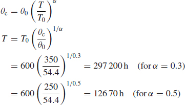
The M(t) method of plotting failure data is a simple and effective way of monitoring reliability changes over time. It is most suitable for analysing the reliability performance of equipment in service. Figure 14.9(a) shows a typical situation in which new equipment is introduced to service over a period (calendar time), and suffer failures which incur down time (repair, delays, etc.). Figure 14.9(b) shows the same population, but now with operating time (calendar time minus down time, or operating hours, as appropriate) as the horizontal scale. The population graph (Figure 14.9(c)) shows the systems at risk as a function of operating time.

M(t) is calculated at each failure from the formula

where: M(t_i) is the value of M at operating time t_i.

Figure 14.8 Duane plot for Example 14.7.

Figure 14.9 The M(t) analysis method (Courtesy J. Møltoft).

Figure 14.9(d) is the M(t) graph. The slope of the line indicates the proportion per time unit failing at that time, or the failure intensity. Reliability improvement (either due to a decreasing instantaneous failure rate pattern or to reliability improvement actions) will reduce the slope. A straight line indicates a constant (random) pattern. An increasing slope indicates an increasing pattern, and vice versa Changes in slope indicate changing trends: for example, Figure 14.9(d) is typical of an early ‘infant mortality’ period, caused probably by manufacturing problems, followed by a constant failure intensity. The failure intensity over any period can be calculated by measuring the slope. The proportions failing over a period can be determined by reading against the M(t) scale.

The M(t) method can be used to monitor reliability trends such as the effectiveness of improvement actions. Example 14.8 illustrates this.

Example 14.8

Table 14.5 shows data on systems in service. Figure 14.10a and Figure 14.10b show Δ r(t) and N(t) respectively, and Figure 14.10c is the M(t) plot.

From the M(t) graph we can determine that:

1. Over the first 400 h no failures occur, but then failures occur at a fairly high and increasing intensity thereafter. This could indicate a failure-free period for the population.
2. The failure intensity continues at a roughly constant level (about 2.5 failures/unit/1000 h), until 1400 h, when it drops to about 1 failure/unit/1000 h. This might be due to the weeding out of the flaws (latent defects) in the systems, modification to units in service, improved maintenance, and so on.
3. By extrapolating the asymptotic part of the curve back to the M(t) axis, we see that on average each system has failed and been repaired about twice.

The M(t) method can be useful for identifying and interpreting failure trends. It can also be used for evaluating logistics and warranty policies. For example, if the horizontal scale represents calendar time, the expected number of failures over selected periods can be determined by reading the intercepts on the M(t) scale (e.g. in Example 14.8 a linear extrapolation of the final slope would indicate about 1 failure/unit/1000 h of the matured systems and about 12% flaws). The method is described in Møltoft (1994).

Table 14.5 Service data.

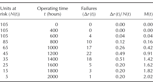
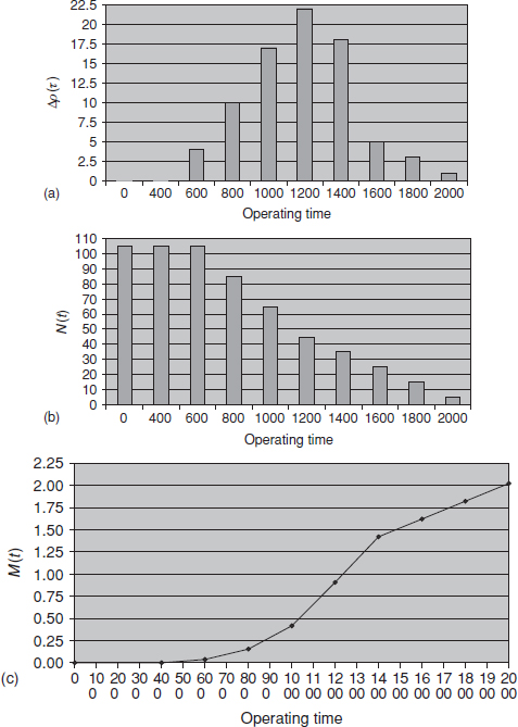
Figure 14.10 M(t) graph of Table 14.5.

14.13.3 Reliability Growth Estimation by Failure Data Analysis

Reliability growth can be estimated by considering the failure data and the planned corrective action. No empirical model is used and the method takes direct account of what is known and planned, so it can be easier to sell. However, it can only be applied when sufficient data are available, well into a development programme or when the product is in service.

If we know that 20% of failures are caused by failure modes for which corrective action is planned and we are sure that the changes will be effective, we can simply estimate that the improvement in failure rate will be 20%. Alternatively, we could assign an effectiveness value to the changes, say 80%, in which case the failure rate improvement will be 16%.

This approach should be used whenever failure data and failure investigations are comprehensive enough to support a Pareto analysis, as described in Section 13.2. The method can be used in conjunction with a Duane plot. If known failure modes can be corrected, reliability growth can be anticipated. However, if reliability is below target and no corrective action is planned, the reliability growth forecast will not have much meaning.

14.14 Making Reliability Grow

In this chapter we have covered methods for measuring reliability achievement and growth. Of course it is not enough just to measure performance. Effort must be directed towards maximizing reliability. In reliability engineering this means taking positive action to unearth design and production shortfalls which can lead to failure, to correct these deficiencies and to prove that the changes are effective. In earlier chapters we have covered the methods of stress analysis, design review, testing and failure data analysis which can be used to ensure a product's reliability. To make these activities as effective as possible, it is necessary to ensure that they are all directed towards the reliability achievement which has been specified.

There is a dilemma in operating such a programme. There will be a natural tendency to try to demonstrate that the reliability requirements have been met. This can lead to reluctance to induce failures by increasing the severity of tests and to a temptation to classify failures as non-relevant or unlikely to recur. On the other hand, reliability growth is maximized by deliberate and aggressive stress-testing, analysis and corrective action as described in Chapter 12. Therefore, the objective should be to stimulate failures during development testing and not to devise tests and failure-reporting methods whose sole objective is to maximize the chances of demonstrating that a specification has been satisfied. Such an open and honest programme makes high demands on teamwork and integrity, and emphasizes the importance of the project manager understanding the aims and being in control of the reliability programme.¹ The reliability milestones should be stated early in the programme and achievement should be monitored against this statement.

14.14.1 Test, Analyse and Fix

Reliability growth programmes as described above have come to be known as test, analyse and fix (TAAF). It is very important in such programmes that:

1. All failures are analysed fully, and action taken in design or production to ensure that they should not recur. No failure should be dismissed as being ‘random’ or ‘non-relevant’ during this stage, unless it can be demonstrated conclusively that such a failure cannot occur on production units in service.
2. Corrective action must be taken as soon as possible on all units in the development programme. This might mean that designs have to be altered more often, and can cause programme delays. However, if faults are not corrected reliability growth will be delayed, potential failure modes at the ‘next weakest link’ may not be highlighted, and the effectiveness of the corrective action will not be adequately tested.

Action on failures should be based on a disciplined FRACAS (Section 12.6) and Appendix 5.

Whenever failures occur, the investigation should refer back to the reliability predictions, stress analyses and FMECAs to determine if the analyses were correct. Discrepancies should be noted and corrected to aid future work of this type.

14.14.2 Reliability Growth in Service

The same principles as described above should be applied to reliability growth in service. However, there are three main reasons why in-service reliability growth is more difficult to achieve than during the development phase:

1. Failure data are often more difficult to obtain. Warranty or service contract repair reports are a valuable source of reliability data, but they are often harder to control, investigation can be more difficult with equipment in the users’ hands and data often terminate at the end of the warranty period. (Use of warranty data was covered in detail in Chapter 13). Some companies make arrangements with selected dealers to provide comprehensive service data. Military and other government customers often operate their own in-use failure data systems. However, in-use data very rarely match the needs of a reliability growth programme.
2. It is much more difficult and much more expensive to modify delivered equipment or to make changes once production has started.
3. A product's reputation is made by its early performance. Reliance on reliability growth in use can be very expensive in terms of warranty costs, reputation and markets.

Nevertheless, a new product will often have in-service reliability problems despite an intensive development programme. Therefore reliability data must be collected and analysed, and improvements designed and implemented. Most products which deserve a reliability programme have a long life in service and undergo further evolutionary development, and therefore a continuing reliability improvement programme is justifiable. When evolutionary development takes place in-use data can be a valuable supplement to further reliability test data, and can be used to help plan the follow-on development and test programme. The FRACAS described in Appendix 5 can be used for in-service failures.

Another source of reliability data is that from production test and inspection. Many products are tested at the end of the production line and this includes burn-in for many types of electronic equipment. Whilst data from production test and inspection are collected primarily to monitor production quality costs and vendor performance, they can be a useful supplement to in-use reliability data. Also, as the data collection and the product are still under the manufacturer's control, faster feedback and corrective action can be accomplished.

The manufacturer can run further tests of production equipment to verify that reliability and quality standards are being maintained. Such tests are often stipulated as necessary for batch release in government production contracts. As in-house tests are under the manufacturer's control, they can provide early warning of incipient problems and can help to verify that the reliability of production units is being maintained or improved.

Questions

1. Compare the B₅-life of 10 years and MTBF = 150 years. Which metric gives the higher reliability at 10 years?
2. How many test units are required to demonstrate 97.5% reliability at 50% confidence if no failures are allowed?
3. You are planning to conduct a success run test with 50 samples:
   1. What reliability can you demonstrate with 90% confidence?
   2. What would be your demonstrated reliability if during the test you experience two failures?
4. The cost of product validation is $ 1600 per test sample (includes the cost to produce, test, monitor and analyse the unit). How much extra cost will be incurred if the reliability demonstration requirement changes from R = 95.0% to 97.0% at the same 90% confidence level?
5. Reliability specification calls for reliability demonstration of R = 95.0% with the confidence C = 90%. The accelerated thermal cycling test equivalent to one field life consists of 1000 cycles. Calculate the following:
   1. How many samples need to be tested without failures in order to meet this requirement?
   2. If your chamber can only fit 30 units, how many cycles you would need to run to meet this requirement with this quantity of units? From the past test experience with this product you know the Weibull slope β = 2.5.
6. Three electric transformers were tested under high temperature and humidity conditions. The test units were inspected at the beginning of the test (time = 0), at 500 hours, and at the end of the test (time = 1000 hours). The unit is considered failed if the inductance falls below 32 μH. The inductance values are presented below:

   

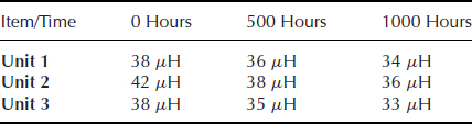
   Determine:

   1. The expected failure times for each unit using the linear extrapolation.
   2. Conduct life data analysis (2-parameter Weibull) and determine β and η parameters.
   3. Calculate the B₁₀ life.
   4. Explore the exponential and power extrapolations. Compare with the results obtained in (a), (b) and (c).
7. 1. Explain why and under what circumstances it might be valid to assume the exponential distribution for interfailure times of a complex repairable system even though it may contain ‘wearout’ components.
   2. Such a system has, on test, accumulated 1053 h of running during which there have been two failures. Estimate the MTBF of the system, and its lower 90% confidence limit.
   3. On the assumption that no more failures occur, how much more testing is required to demonstrate with 90% confidence that the true MTBF is not less than 500 h? Comment on the implications of your answer.
8. 1. In a complex repairable system 1053 h of testing have been accumulated, with failures at 334 h and 891 h. Assuming constant failure rate, calculate (i) the current estimate of the system failure rate; (ii) the current estimate of the mean time between failures (MTBF); and (iii) the lower 90% confidence limit for the MTBF.
   2. For the above system, if there is a specification requirement that the MTBF shall be at least 500 h, and this must be demonstrated at 90% confidence, how much more test running of the system, without further failure, is required?
9. Five engines are tested to failure. Failure times are 628 hours, 3444 hours, 822 hour, 846 hours, and 236 hours. Assuming a constant failure rate, what is the two-sided 90% confidence interval for the MTBF?
10. You are running a continuous operation of five turbines for 1000 hours. During that test one turbine has failed at 825 hours and was removed from the test. What is the one-sided 90% confidence limit on the failure rate?
11. Explain the principles of probability ratio sequential testing (PRST) to demonstrate MTBF. What are the main limitations of the method?
12. Explain what is the design ratio in PRST? How is it linked with the risks and the expected test duration?
13. If a Duane growth model has a slope of 0.4 with a cumulative MTBF of 40 000 hours, what is the instantaneous MTBF?
14. What is the major contributor to reliability growth and continuous product and process improvement?
15. A prototype of a repairable system was subjected to a test programme where engineering action is supposedly taken to eliminate causes of failure as they occur. The first 500 h of running gave failures at 12, 36, 80, 120, 200, 360, 400, 440 and 480 hours:
    1. Use a Duane plot to discover whether reliability growth is occurring.
    2. Calculate the trend statistic (Eq. 2.46) and see whether it gives results consistent with (a).

Bibliography

British Standard, BS 5760. Reliability of Systems, Equipments and Components, Part 2. British Standards Institution, London.

Kleyner, A. and Boyle, J. (2004) The Myths of Reliability Demonstration Testing! TEST Engineering and Management, August/ September 2004, pp. 16–17.

Kleyner, A., Bhagath, S., Gasparini, M. et al. (1997) Bayesian Techniques to Reduce the Sample Size in Automotive Electronics Attribute Testing. Microelectronics and Reliability, 37(6), 879–883.

Lipson, C. and Sheth, N. (1973) Statistical Design and Analysis of Engineering Experiments, McGraw-Hill.

Møltoft, J. (1994) Reliability Engineering Based on Field Information: The Way Ahead. Quality and Reliability Engineering International, 10, 399–409.

ReliaSoft (2006) Degradation Analysis. Web reference. Available at: http://www.weibull.com/LifeDataWeb/degradation_analysis.htm.

US MIL-HDBK-781. Reliability Testing for Equipment Development, Qualification and Production. Available from the National Technical Information Service, Springfield, Virginia.

Wasserman, G. (2003) Reliability Verification, Testing, and Analysis in Engineering Design, Marcel Dekker.

Yates, S. (2008) Australian Defense Standard for Bayesian Reliability Demonstration. Proceedings of the Annual Reliability and Maintainability Symposium (RAMS), pp. 103–107.