2

Reliability Mathematics

2.1 Introduction

The methods used to quantify reliability are the mathematics of probability and statistics. In reliability work we are dealing with uncertainty. As an example, data may show that a certain type of power supply fails at a constant average rate of once per 10⁷ h. If we build 1000 such units, and we operate them for 100 h, we cannot say with certainty whether any will fail in that time. We can, however, make a statement about the probability of failure. We can go further and state that, within specified statistical confidence limits, the probability of failure lies between certain values above and below this probability. If a sample of such equipment is tested, we obtain data which are called statistics.

Reliability statistics can be broadly divided into the treatment of discrete functions, continuous functions and point processes. For example, a switch may either work or not work when selected or a pressure vessel may pass or fail a test—these situations are described by discrete functions. In reliability we are often concerned with two-state discrete systems, since equipment is in either an operational or a failed state. Continuous functions describe those situations which are governed by a continuous variable, such as time or distance travelled. The electronic equipment mentioned above would have a reliability function in this class. The distinction between discrete and continuous functions is one of how the problem is treated, and not necessarily of the physics or mechanics of the situation. For example, whether or not a pressure vessel fails a test may be a function of its age, and its reliability could therefore be treated as a continuous function. The statistics of point processes are used in relation to repairable systems, when more than one failure can occur in a time continuum. The choice of method will depend upon the problem and on the type of data available.

2.2 Variation

Reliability is influenced by variability, in parameter values such as resistance of resistors, material properties, or dimensions of parts. Variation is inherent in all manufacturing processes, and designers should understand the nature and extent of possible variation in the parts and processes they specify. They should know how to measure and control this variation, so that the effects on performance and reliability are minimized.

Variation also exists in the environments that engineered products must withstand. Temperature, mechanical stress, vibration spectra, and many other varying factors must be considered.

Statistical methods provide the means for analysing, understanding and controlling variation. They can help us to create designs and develop processes which are intrinsically reliable in the anticipated environments over their expected useful lives.

Of course, it is not necessary to apply statistical methods to understand every engineering problem, since many are purely deterministic or easily solved using past experience or information available in sources such as databooks, specifications, design guides, and in known physical relationships such as Ohm's law. However, there are also many situations in which appropriate use of statistical techniques can be very effective in optimizing designs and processes, and for solving quality and reliability problems.

2.2.1 A Cautionary Note

Whilst statistical methods can be very powerful, economic and effective in reliability engineering applications, they must be used in the knowledge that variation in engineering is in important ways different from variation in most natural processes, or in repetitive engineering processes such as repeated, in-control machining or diffusion processes. Such processes are usually:

• Constant in time, in terms of the nature (average, spread, etc.) of the variation.
• Distributed in a particular way, describable by a mathematical function known as the normal distribution (which will be described later in this chapter).

In fact, these conditions often do not apply in engineering. For example:

• A component supplier might make a small change in a process, which results in a large change (better or worse) in reliability. The change might be deliberate or accidental, known or unknown. Therefore the use of past data to forecast future reliability, using purely statistical methods, might be misleading.
• Components might be selected according to criteria such as dimensions or other measured parameters. This can invalidate the normal distribution assumption on which much of the statistical method is based. This might or might not be important in assessing the results.
• A process or parameter might vary in time, continuously or cyclically, so that statistics derived at one time might not be relevant at others.
• Variation is often deterministic by nature, for example spring deflection as a function of force, and it would not always be appropriate to apply statistical techniques to this sort of situation.
• Variation in engineering can arise from factors that defy mathematical treatment. For example, a thermostat might fail, causing a process to vary in a different way to that determined by earlier measurements, or an operator or test technician might make a mistake.
• Variation can be discontinuous. For example, a parameter such as a voltage level may vary over a range, but could also go to zero.

These points highlight the fact that variation in engineering is caused to a large extent by people, as designers, makers, operators and maintainers. The behaviour and performance of people is not as amenable to mathematical analysis and forecasting as is, say, the response of a plant crop to fertilizer or even weather patterns to ocean temperatures. Therefore the human element must always be considered, and statistical analysis must not be relied on without appropriate allowance being made for the effects of factors such as motivation, training, management, and the many other factors that can influence reliability.

Finally, it is most important to bear in mind, in any application of statistical methods to problems in science and engineering, that ultimately all cause and effect relationships have explanations, in scientific theory, engineering design, process or human behaviour, and so on. Statistical techniques can be very useful in helping us to understand and control engineering situations. However, they do not by themselves provide explanations. We must always seek to understand causes of variation, since only then can we really be in control. See the quotations on the flyleaf, and think about them.

2.3 Probability Concepts

Any event has a probability of occurrence, which can be in the range 0–1. A zero probability means that the event will not occur; a probability of 1 means that it will occur. A coin has a 0.5 (even) probability of landing heads, and a die has a 1/6 probability of giving any one of the six numbers. Such events are independent, that is, the coin and the die logically have no memory, so whatever has been thrown in the past cannot affect the probability of the next throw. No ‘system’ can beat the statistics of these situations; waiting for a run of blacks at roulette and then betting on reds only appears to work because the gamblers who won this way talk about it, whilst those who lost do not.

With coins, dice and roulette wheels we can predict the probability of the outcome from the nominal nature of the system. A coin has two sides, a die six faces, a roulette wheel equal numbers of reds and blacks. Assuming that the coin, die and wheel are fair, these outcomes are also unbiased, that is, they are all equally probable. In other words, they occur randomly.

With many systems, such as the sampling of items from a production batch, the probabilities can only be determined from the statistics of previous experience.

We can define probability in two ways:

1. If an event can occur in N equally likely ways, and if the event with attribute A can happen in n of these ways, then the probability of A occurring is

   

2. If, in an experiment, an event with attribute A occurs n times out of N experiments, then as n becomes large, the probability of event A approaches n/N, that is,

   

   The first definition covers the cases described earlier, that is, equally likely independent events such as rolling dice. The second definition covers typical cases in quality control and reliability. If we test 100 items and find that 30 are defective, we may feel justified in saying that the probability of finding a defective item in our next test is 0.30, or 30%.

However, we must be careful in making this type of assertion. The probability of 0.30 of finding a defective item in our next test may be considered as our degree of belief, in this outcome, limited by the size of the sample. This leads to a third, subjective, definition of probability. If, in our tests of 100 items, seven of the defectives had occurred in a particular batch of ten and we had taken corrective action to improve the process so that such a problem batch was less likely to occur in future, we might assign some lower probability to the next item being defective. This subjective approach is quite valid, and is very often necessary in quality control and reliability work. Whilst it is important to have an understanding of the rules of probability, there are usually so many variables which can affect the properties of manufactured items that we must always keep an open mind about statistically derived values. We must ensure that the sample from which statistics have been derived represents the new sample, or the overall population, about which we plan to make an assertion based upon our sample statistics.

Figure 2.1 Samples with defectives (black squares).

A sample represents a population if all the members of the population have an equal chance of being sampled. This can be achieved if the sample is selected so that this condition is fulfilled. Of course in engineering this is not always practicable; for example, in reliability engineering we often need to make an assertion about items that have not yet been produced, based upon statistics from prototypes.

To the extent that the sample is not representative, we will alter our assertions. Of course, subjective assertions can lead to argument, and it might be necessary to perform additional tests to obtain more data to use in support of our assertions. If we do perform more tests, we need to have a method of interpreting the new data in relation to the previous data: we will cover this aspect later.

The assertions we can make based on sample statistics can be made with a degree of confidence which depends upon the size of the sample. If we had decided to test ten items after introducing a change to the process, and found one defective, we might be tempted to assert that we have improved the process, from 30% defectives being produced to only 10%. However, since the sample is now much smaller, we cannot make this assertion with as high confidence as when we used a sample of 100. In fact, the true probability of any item being defective might still be 30%, that is, the population might still contain 30% defectives.

Figure 2.1 shows the situation as it might have occurred, over the first 100 tests. The black squares indicate defectives, of which there are 30 in our batch of 100. If these are randomly distributed, it is possible to pick a sample batch of ten which contains fewer (or more) than three defectives. In fact, the smaller the sample, the greater will be the sample-to-sample variation about the population average, and the confidence associated with any estimate of the population average will be accordingly lower. The derivation of confidence limits is covered later in this chapter.

2.4 Rules of Probability

In order to utilize the statistical methods used in reliability engineering, it is necessary to understand the basic notation and rules of probability. These are:

1. The probability of obtaining an outcome A is denoted by P(A), and so on for other outcomes.
2. The joint probability that A and B occur is denoted by P(AB).
3. The probability that A or B occurs is denoted by P(A + B).
4. The conditional probability of obtaining outcome A, given that B has occurred, is denoted by P(A | B).
5. The probability of the complement, that is, of A not occurring, is P(Ā) = 1 – P(A)
6. If (and only if) events A and B are independent, then

   

   and

   

   that is, P(A) is unrelated to whether or not B occurs, and vice versa.

7. The joint probability of the occurrence of two independent events A and B is the product of the individual probabilities:

   

   This is also called the product rule or series rule. It can be extended to cover any number of independent events. For example, in rolling a die, the probability of obtaining any given sequence of numbers in three throws is

   

8. If events A and B are dependent, then

   

   that is, the probability of A occurring times the probability of B occurring given that A has already occurred, or vice versa.

   If P(A) ≠ 0, (2.3) can be rearranged to

   

9. The probability of any one of two events A or B occurring is

   

10. The probability of A or B occurring, if A and B are independent, is

    

    The derivation of this equation can be shown by considering the system shown in Figure 2.2, in which either A or B, or A and B, must work for the system to work. If we denote the system success probability as P_s, then the failure probability, P_f = 1 – P_s. The system failure probability is the joint probability of A and B failing, that is,

    

11. If events A and B are mutually exclusive, that is, A and B cannot occur simultaneously, then

    

    and

    

12. If multiple, mutually exclusive probabilities of outcomes B_i jointly give a probability of outcome A, then

    

13. Rearranging Eq. (2.3)

    

    we obtain

    

    This is a simple form of Bayes' theorem. A more general expression is

    

where E_i is the ith event.

Figure 2.2 Dual redundant system.

Example 2.1

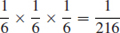
The reliability of a missile is 0.85. If a salvo of two missiles is fired, what is the probability of at least one hit? (Assume independence of missile hits.)

Let A be the event ‘first missile hits’ and B the event ‘second missile hits’. Then

There are four possible, mutually exclusive outcomes, AB, A, ĀB; Ā. The probability of both missing, from Eq. (2.2), is

Therefore the probability of at least one hit is

We can derive the same result by using Eq. (2.6):

Another way of deriving this result is by using the sequence tree diagram:

The probability of a hit is then derived by summing the products of each path which leads to at least one hit. We can do this since the events defined by each path are mutually exclusive.

(Note that the sum of all the probabilities is unity.)

Example 2.2

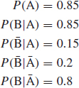
In Example 2.1 the missile hits are not independent, but are dependent, so that if the first missile fails the probability that the second will also fail is 0.2. However, if the first missile hits, the hit probability of the second missile is unchanged at 0.85. What is the probability of at least one hit?

The probability of at least one hit is

Since A, B and A are independent,

and

Since Ā and B are dependent, from Eq. (2.3),

and the sum of these probabilities is 0.97.

This result can also be derived by using a sequence tree diagram:

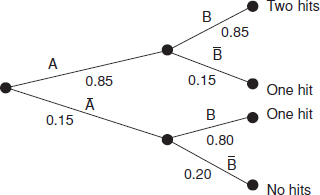
As in Example 2.1, the probability of at least one hit is calculated by adding the products of each path leading to at least one hit, that is,

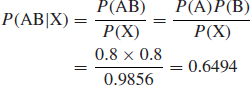
Example 2.3

In the circuit shown, the probability of any switch being closed is 0.8 and all events are independent. (a) What is the probability that a circuit will exist? (b) Given that a circuit exists, what is the probability that switches a and b are closed?

Let the events that a, b, c and d are closed be A, B, C and D. Let X denote the event that the circuit exists.

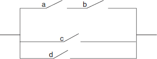
(a) X = AB + (C + D)

Therefore

P(X) = 0.64 + 0.96 − (0.96 × 0.64) = 0.9856

(b)From Eq. (2.4),

A and B jointly give X. Therefore, from Eq. (2.8),

P(ABX) = P(AB)

So

Example 2.4

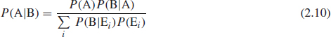
A test set has a 98% probability of correctly classifying a defective item and a 4% probability of classifying a good item as defective. If in a batch of items tested 3% are actually defective, what is the probability that when an item is classified as defective, it is truly defective?

Let D represent the event that an item is defective and C represent the event that an item is classified defective. Then

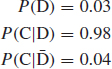
We need to determine P(D|C). Using Eq. (2.10),

This indicates the importance of a test equipment having a high probability of correctly classifying good items as well as bad items.

More practical applications of the Bayesian statistical approach to reliability can be found in Martz and Waller (1982) or Kleyner et al. (1997).

2.5 Continuous Variation

The variation of parameters in engineering applications (machined dimensions, material strengths, transistor gains, resistor values, temperatures, etc.) are conventionally described in two ways. The first, and the simplest, is to state maximum and minimum values, or tolerances. This provides no information on the nature, or shape, of the actual distribution of values. However, in many practical cases, this is sufficient information for the creation of manufacturable, reliable designs.

The second approach is to describe the nature of the variation, using data derived from measurements. In this section we will describe the methods of statistics in relation to describing and controlling variation in engineering.

If we plot measured values which can vary about an average (e.g. the diameters of machined parts or the gains of transistors) as a histogram, for a given sample we may obtain a representation such as Figure 2.3(a).

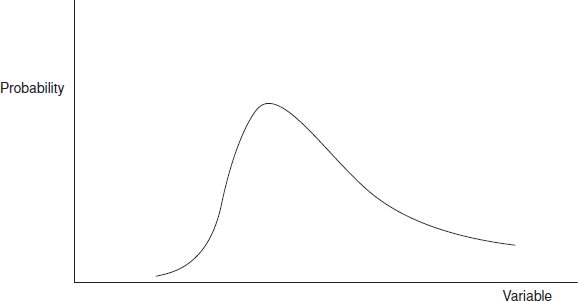
In this case 30 items have been measured and the frequencies of occurrence of the measured values are as shown. The values range from 2 to 9, with most items having values between 5 and 7. Another random sample of 30 from the same population will usually generate a different histogram, but the general shape is likely to be similar, for example, Figure 2.3(b). If we plot a single histogram showing the combined data of many such samples, but this time show the values in measurement intervals of 0.5, we get Figure 2.3(c). Note that now we have used a percentage frequency scale. We now have a rather better picture of the distribution of values, as we have more information from the larger sample. If we proceed to measure a large number and we further reduce the measurement interval, the histogram tends to a curve which describes the population probability density function (pdf) or simply the distribution of values. Figure 2.4 shows a general unimodal probability distribution, f(x) being the probability density of occurrence, related to the variable x. The value of x at which the distribution peaks is called the mode. Multimodal distributions are encountered in reliability work as well as unimodal distributions. However, we will deal only with the statistics of unimodal distributions in this book, since multimodal distributions are usually generated by the combined effects of separate unimodal distributions.

Figure 2.3 (a) Frequency histogram of a random sample, (b) frequency histogram of another random sample from the same population, (c) data of many samples shown with measurement intervals of 0.5.

The area under the curve is equal to unity, since it describes the total probability of all possible values of x, as we have defined a probability which is a certainty as being a probability of one. Therefore

The probability of a value falling between any two values x₁ and x₂ is the area bounded by this interval, that is,

To describe a pdf we normally consider four aspects:

1. The central tendency, about which the distribution is grouped.
2. The spread, indicating the extent of variation about the central tendency.
3. The skewness, indicating the lack of symmetry about the central tendency. Skewness equal to zero is a characteristic of a symmetrical distribution. Positive skewness indicates that the distribution has a longer tail to the right (see for example Figure 2.5) and negative skewness indicates the opposite.

   

   Figure 2.4 Continuous probability distribution.

   

   Figure 2.5 Measures of central tendency.

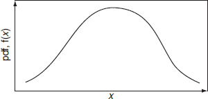
4. The kurtosis, indicating the ‘peakedness’ of the pdf In general terms kurtosis characterizes the relative peakedness or flatness of a distribution compared to the normal distribution. Positive kurtosis indicates a relatively peaked distribution. Negative kurtosis indicates a relatively flat distribution.

2.5.1 Measures of Central Tendency

For a sample containing n items the sample mean is denoted by :

The sample mean can be used to estimate the population mean, which is the average of all possible outcomes. For a continuous distribution, the mean is derived by extending this idea to cover the range −∞ to + ∞.

The mean of a distribution is usually denoted by μ. The mean is also referred to as the location parameter, average value or expected value, E(x).

This is analogous to the centre of gravity of the pdf The estimate of a population mean from sample data is denoted by .

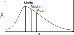
Other measures of central tendency are the median, which is the mid-point of the distribution, that is, the point at which half the measured values fall to either side, and the mode, which is the value (or values) at which the distribution peaks. The relationship between the mean, median and mode for a right-skewed distribution is shown in Figure 2.5. For a symmetrical distribution, the three values are the same, whilst for a left-skewed distribution the order of values is reversed.

2.5.2 Spread of a Distribution

The spread, or dispersion, that is, the extent to which the values which make up the distribution vary, is measured by its variance. For a sample size n the variance, Var (x) or E(x – )², is given by

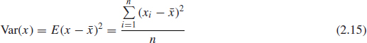
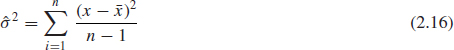
Where sample variance is used to estimate the population variance, we use (n – 1) in the denominator of Eq. (2.15) instead of n, as it can be shown to provide a better estimate. The estimate of population variance from a sample is denoted ² where

The population variance σ², for a finite population N, is given by

For a continuous distribution it is:

σ is called the standard deviation (SD) and is frequently used in practice instead of the variance. It is also referred to as the scale parameter. σ² is the second moment about the mean and is analogous to a radius of gyration.

The third and fourth moments about the mean give the skewness and kurtosis mentioned before. Since we will not make use of these parameters in this book, the reader is referred to more advanced statistical texts for their derivation (e.g. Hines and Montgomery, 1990).

2.5.3 The Cumulative Distribution Function

The cumulative distribution function (cdf), F(x), gives the probability that a measured value will fall between −∞ and x:

Figure 2.6 shows the typical ogive form of the cdf with F(x) → 1 as x → ∞.

Figure 2.6 Typical cumulative distribution function (cdf).

2.5.4 Reliability and Hazard Functions

In reliability engineering we are concerned with the probability that an item will survive for a stated interval (e.g. time, cycles, distance, etc.), that is, that there is no failure in the interval (0 to x). This is the reliability, and it is given by the reliability function R(x). From this definition, it follows that

The hazard function or hazard rate h(x) is the conditional probability of failure in the interval x to (x + dx), given that there was no failure by x:

The cumulative hazard function H(x) is given by

Figure 2.7 illustrates the relationship between the failure probability density function (pdf), reliability R(t), and failure function F(t). At any point of time the area under the curve left of t would represent the fraction of the population expected to fail F(t) and area to the right the fraction expected to survive R(t).

Please note, that in engineering we do not usually encounter measured values below zero and the lower limit of the definite integral is then 0.

2.5.5 Calculating Reliability Using Microsoft Excel¯ Functions

In the past decades the Microsoft Excel¯ spreadsheet software became a widely utilized tool to perform a multitude of engineering and non-engineering tasks including statistical calculations. This book will illustrate how to perform some statistical analysis including reliability calculations utilizing Excel spreadsheet functions. Excel applications will cover both continuous and discrete statistical distributions.

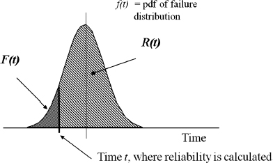
Figure 2.7 Probability Density Function (pdf) and its application to reliability.

2.6 Continuous Distribution Functions

2.6.1 The Normal (or Gaussian) Distribution

By far the most widely used ‘model’ of the nature of variation is the mathematical function known as the normal (or Gaussian) distribution. The normal data distribution pattern occurs in many natural phenomena, such as human heights, weather patterns, and so on. However, there are limitations inherent in using this model in many engineering applications (see the comments in Section 2.8.1).

The normal pdf is given by

where μ is the location parameter, equal to the mean. The mode and the median are coincident with the mean, as the pdf is symmetrical. σ is the scale parameter, equal to the SD.

A population which conforms to the normal distribution has variations which are symmetrically disposed about the mean (Figure 2.8) (i.e. the skewness is zero). Since the tails of the normal distribution are symmetrical, a given spread includes equal values in the left-hand and right-hand tails.

For normally distributed variables, about 68% of the population fall between ± 1 SD. About 95% fall between ± 2 SD, and about 99.7% between ± 3 SD.

An important reason for the wide applicability of the normal distribution is the fact that, whenever several random variables are added together, the resulting sum tends to normal regardless of the distributions of the variables being added. This is known as the central limit theorem. It justifies the use of the normal distribution in many engineering applications, including quality control. The normal distribution is a close fit to most quality control and some reliability observations, such as the sizes of machined parts and the lives of items subject to wearout failures. Appendix 1 gives values for Φ(z), the standardized normal cdf, that is, μ = 0 and σ = 1. z represents the number of SDs displacement from the mean. Any normal distribution can be evaluated from the standardized normal distribution by calculating the standardized normal variate z, where

Figure 2.8 The normal (Gaussian) distribution.

and finding the appropriate value of Φ (z).

The pdf of a normal distribution with parameters μ and σ can be calculated using Excel as f(x) = NORMDIST(x, μ, σ, FALSE) and reliability as R(x) =1-NORMDIST(x, μ, σ, TRUE). The standardized normal cdf can be calculated as Φ (z) = NORMSDIST(z).

Example 2.5

The life of an incandescent lamp is normally distributed, with mean 1200 h and SD 200 h. What is the probability that a lamp will last (a) at least 800 h? (b) at least 1600 h?

a z (x – μ)/σ, that is, the distance of x from μ expressed as a number of SDs. Then

Appendix 1 shows that the probability of a value not exceeding 2 SD is 0.977. Figure 2.9(a) shows this graphically, on the pdf (the shaded area).

b The probability of a lamp surviving more than 1600 h is derived similarly:

This represents the area under the pdf curve beyond the +2 SD point. (Figure 2.9(a)) or 1− (area under the curve to the left of +2 SD) on the cdf (Figure 2.9(b)). Therefore the probability of surviving beyond 1600h is (1 - 0.977) = 0.023.

The answers can also be obtained using Excel functions as follows:

Figure 2.9 (a) The pdf f(x) versus x; (b) the cdf F(x) versus x (see Example 2.5).

2.6.2 The Lognormal Distribution

The lognormal distribution is based on the normal distribution. A random variable is lognormally distributed if the logarithm of the random variable is normally distributed. The lognormal distribution is a more versatile distribution than the normal as it has a range of shapes, and therefore is often a better fit to reliability data, such as for populations with wearout characteristics. Also, it does not have the normal distribution's disadvantage of extending below zero to −∞. Outside reliability applications the lognormal is often used to model usage data, such as vehicle mileage per year, count of switch operations, repair time of a maintained system, and so on. The lognormal pdf is

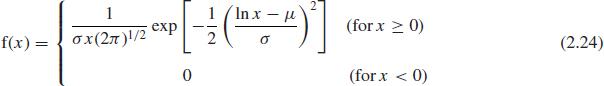
As mentioned before, it is the normal distribution with ln x as the variate. The mean and SD of the lognormal distribution are given by

where μ and σ are the mean and SD of the ln data.

When μ » σ, the lognormal distribution approximates to the normal distribution. The normal and lognormal distributions describe reliability situations in which the hazard rate increases from x = 0 to a maximum and then decreases.

The cdf and reliability of the system following lognormal distribution with parameters μ and σ can also be calculated using Excel functions.

For example, R(x) = 1-LOGNORMDIST(x, μ, σ).

2.6.3 The Exponential Distribution

The exponential distribution describes the situation wherein the hazard rate is constant. A Poisson process (Section 2.10.2) generates a constant hazard rate. The pdf is

This is an important distribution in reliability work, as it has the same central limiting relationship to life statistics as the normal distribution has to non-life statistics. It describes the constant hazard rate situation. As the hazard rate is often a function of time, we will denote the independent variable by t instead of x. The constant hazard rate is denoted by λ. The mean life, or mean time to failure (MTTF), is 1/λ. The pdf is then written as

The probability of no failures occurring before time t is obtained by integrating Eq. (2.26) between 0 and t and subtracting from 1:

The Excel functions for the exponential distribution are: pdf f(t) = EXPONDIST(t, λ, FALSE) and reliability R(t) =1-EXPONDIST(t, λ, TRUE).

R(t) is the reliability function (or survival probability). For example, the reliability of an item with an MTTF of 500 h over a 24 h period is

For items which are repaired, λ is called the failure rate, and 1/λ is called the mean time between failures (MTBF) (also referred as θ). Please note from Eq. (2.27) that 63.2% of items will have failed by t = MTBF.

2.6.4 The Gamma Distribution

In statistical terms the gamma distribution represents the sum of n exponentially distributed random variables. The gamma distribution is a flexible life distribution model that may offer a good fit to some sets of failure data. In reliability terms, it describes the situation when partial failures can exist, that is, when a given number of partial failure events must occur before an item fails, or the time to the ath failure when time to failure is exponentially distributed. The pdf is

where λ is the failure rate (complete failures) and a the number of partial failures per complete failure, or events to generate a failure. Γ(a) is the gamma function:

When (a – 1) is a positive integer, Γ(a) = (a – 1)! This is the case in the partial failure situation. The exponential distribution is a special case of the gamma distribution, when a = 1, that is,

The gamma distribution can also be used to describe a decreasing or increasing hazard rate. When a < 1, h(x) will decrease whilst for a > 1, h(x) increases.

Utilizing Excel functions, pdf f(x) = GAMMADIST(x, a, λ, FALSE) and reliability

R(x) = 1-GAMMADIST(x, a, 1, TRUE)

2.6.5 The χ² Distribution

The χ² (chi-square) distribution is a special case of the gamma distribution, where λ = , and v = a/2, where v is called the number of degrees of freedom and must be a positive integer. This permits the use of the χ² distribution for evaluating reliability situations, since the number of failures, or events to failure, will always be positive integers. The χ² distribution is really a family of distributions, which range in shape from that of the exponential to that of the normal distribution. Each distribution is identified by the degrees of freedom.

In statistical theory, the χ² distribution is very important, as it is the distribution of the sums of squares of n, independent, normal variates. This allows it to be used for statistical testing, goodness-of-fit tests and evaluating confidence. These applications are covered later. The cdf for the χ² distribution is tabulated for a range of degrees of freedom in Appendix 2. The Excel function corresponding to Appendix 2 tables is = CHIINV(α, ν) with α being a risk factor.

2.6.6 The Weibull Distribution

The Weibull distribution is arguably the most popular statistical distribution used by reliability engineers. It has the great advantage in reliability work that by adjusting the distribution parameters it can be made to fit many life distributions. When Walloddi Weibull delivered his famous American paper in 1951, the first reaction to his statistical distribution was negative, varying from skepticism to rejection. However the US Air Force recognized the merit of Weibull's method and funded his research until 1975.

The Weibull pdf is (in terms of time t)

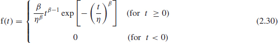
The corresponding reliability function is

The hazard rate is

Mean or MTTF:

Standard deviation:

β is the shape parameter and η is the scale parameter, or characteristic life—it is the life at which 63.2% of the population will have failed (see Eq. (2.31) substituting t = η).

When β = 1, the exponential reliability function (constant hazard rate) results, with

η = mean life (1/λ).

When β < 1, we get a decreasing hazard rate reliability function.

When β > 1, we get an increasing hazard rate reliability function.

When β = 3.5, for example, the distribution approximates to the normal distribution. Thus the Weibull distribution can be used to model a wide range of life distributions characteristic of engineered products. The Excel function for pdf is f(t) = WEIBULL(t, β, η, FALSE) and reliability R(t) = 1-WEIBULL(t, β, η, TRUE).

So far we have dealt with the two-parameter Weibull distribution. If, however, failures do not start at t = 0, but only after a finite time γ, then the Weibull reliability function takes the form

that is, a three-parameter distribution. γ is called the failure free time, location parameter or minimum life. More on the Weibull distribution will be presented in Chapter 3.

2.6.7 The Extreme Value Distributions

In reliability work we are often concerned not with the distribution of variables which describe the bulk of the population but only with the extreme values which can lead to failure. For example, the mechanical properties of a semiconductor wire bond are such that under normal operating conditions good wire bonds will not fracture or overheat. However, extreme high values of electrical load or extreme low values of bond strength can result in failure. In other words, we are concerned with the implications of the tails of the distributions in load–strength interactions. However, we often cannot assume that, because a measured value appears to be, say, normally distributed, that this distribution necessarily is a good model for the extremes. Also, few measurements are likely to have been made at these extremes. Extreme value statistics are capable of describing these situations asymptotically.

Extreme value statistics are derived by considering the lowest or highest values in each of a series of equal samples. For example, consider the sample data in Table 2.1, taken randomly from a common population. The overall data can be plotted as shown in Figure 2.10 as f(x). However, if we plot separately the lowest values and the highest values in each sample, they will appear as g_L(x) and g_H(x). g_L(x) is the extreme value distribution of the lowest extreme whilst g_H(x) is the extreme value distribution of the highest extreme in each sample. For many distributions the distribution of the extremes will be one of three types:

Type I—also known as the extreme value or Gumbel distribution.

Type II—also known as the log extreme value distribution.

Type III—for the lowest extreme values. This is the Weibull distribution.

Table 2.1 Sample data taken randomly from a common population.

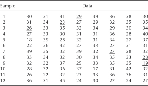
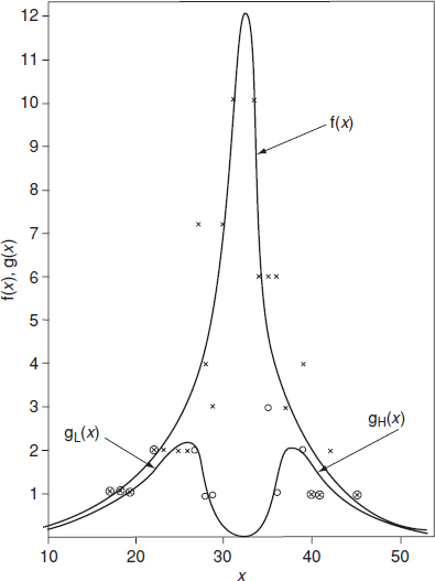
Figure 2.10 Extreme value distributions.

2.6.7.1 Extreme Value Type I

The type I extreme value distributions for maximum and minimum values are the limiting models for the right and left tails of the exponential types of distribution, where this is defined as any distribution whose cumulative probability approaches unity at a rate which is equal to or greater than that for the exponential distribution. This includes most reliability distributions, such as the normal, lognormal and exponential distributions.

The probability density functions for maximum and minimum values, respectively, are

The reduced variate is given by

Substituting in Eqs. (2.33) and (2.34), we can derive the cdf in terms of the reduced variate y. For maximum values:

For minimum values:

The distribution of maximum values is right-skewed and the distribution of minimum values is left-skewed. The hazard function of maximum values approaches unity with increasing x, whilst that for minimum values increases exponentially.

For maximum values:

For minimum values:

The standard deviation μ_ev is 1.283σ in both cases.

2.6.7.2 Extreme Value Type II

The extreme type II distribution does not play an important role in reliability work. If the logarithms of the variables are extreme value distributed, then the variable is described by the extreme value type II distribution. Thus its relationship to the type I extreme value distribution is analogous to that of the lognormal to the normal distribution.

2.6.7.3 Extreme Value Type III

The type III extreme value distribution for minimum values is the limiting model for the left-hand tail for distributions which are bounded at the left. In fact, the Weibull distribution is the type III extreme value distribution for minimum values, and although it was initially derived empirically, its use for describing the strength distribution of materials has been justified using extreme value theory.

2.6.7.4 The Extreme Value Distributions Related to Load and Strength

The type I extreme value distribution for maximum values is often an appropriate model for the occurrence of load events, when these are not bounded to the right, that is, when there is no limiting value.

It is well known that engineering materials possess strengths well below their theoretical capacity, mainly due to the existence of imperfections which give rise to non-uniform stresses under load. In fact, the strength will be related to the effect of the imperfection which creates the greatest reduction in strength, and hence the extreme value distribution for minimum values suggests itself as an appropriate model for strength.

The strength, and hence the time to failure, of many types of product can be considered to be dependent upon imperfections whose extent is bounded, since only very small imperfections will escape detection by inspection or process control, justifying use of a type III (Weibull) model. On the other hand, a type I model might be more representative of the strength of an item which is mass-produced and not 100% inspected, or in which defects can exist whose extent is not bounded, but which are not detected, for example, a long wire, whose strength will then be a function of length.

For a system consisting of many components in series, where the system hazard rate is decreasing from t = 0 (i.e. bounded) a type III (Weibull) distribution will be a good model for the system time to failure.

2.7 Summary of Continuous Statistical Distributions

Figure 2.11 is a summary of the continuous distributions described above.

2.8 Variation in Engineering

Every practical engineering design must take account of the effects of the variation inherent in parameters, environments, and processes. Variation and its effects can be considered in three categories:

1. Deterministic, or causal, which is the case when the relationship between a parameter and its effect is known, and we can use theoretical or empirical formulae, for example, we can use Ohm's law to calculate the effect of resistance change on the performance of a voltage divider. No statistical methods are required. The effects of variation are calculated by inserting the expected range of values into the formulae.
2. Functional, which includes relationships such as the effect of a change of operating procedure, human mistakes, calibration errors, and so on. There are no theoretical formulae. In principle these can be allowed for, but often are not, and the cause and effect relationships are not always easy to identify or quantify.
3. Random. These are the effects of the inherent variability of processes and operating conditions. They can be considered to be the variations that are left unexplained when all deterministic and functional causes have been eliminated. For example, a machining process that is in control will nevertheless produce parts with some variation in dimensions, and random voltage fluctuations can occur on power supplies due to interference. Note that the random variations have causes. However, it is not always possible or practicable to predict how and when the cause will arise. The statistical models described above can be used to describe random variations, subject to the limitations discussed later.

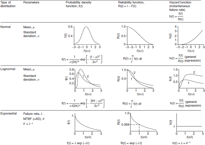
Figure 2.11 Shapes of common failure distributions, reliability and hazard rate functions (shown in relation to t).

Variation can also be progressive, for example due to wear, material fatigue, change of lubricating properties, or electrical parameter drift.

2.8.1 Is the Variation Normal?

The central limit theorem, and the convenient properties of the normal distribution, are the reasons why this particular function is taught as the basis of nearly all statistics of continuous variation. It is a common practice, in most applications, to assume that the variation being analysed is normal, then to determine the mean and SD of the normal distribution that best fits the data.

However, at this point we must stress an important limitation of assuming that the normal distribution describes the real variation of any process. The normal pdf has values between +∞ and −∞. Of course a machined component dimension cannot vary like this. The machine cannot add material to the component, so the dimension of the stock (which of course will vary, but not by much) will set an upper limit. The nature of the machining process, using gauges or other practical limiting features, will set a lower limit. Therefore the variation of the machined dimension would more realistically look something like Figure 2.12. Only the central part might be approximately normal, and the distribution will have been curtailed. In fact all variables, whether naturally occurring or resulting from engineering or other processes, are curtailed in some way, so the normal distribution, while being mathematically convenient, is actually misleading when used to make inferences well beyond the range of actual measurements, such as the probability of meeting an adult who is 1 m tall.

There are other ways in which variation in engineering might not be normal. These are:

• There might be other kinds of selection process. For example, when electronic components such as resistors, microprocessors, and so on are manufactured, they are all tested at the end of the production process. They are then ‘binned’ according to the measured values. Typically, resistors that fall within ±2% of the nominal resistance value are classified as precision resistors, and are labelled, binned and sold as such. Those that fall outside these limits, but within ±10% become non-precision resistors, and are sold at a lower price. Those that fall outside ±10% are scrapped. Because those sold as ±10% will not include any that are ±2%, the distribution of values is as shown in Figure 2.13. Similarly, microprocessors are sold with different operating speeds depending on the maximum speed at which they function correctly on test, having all been produced on the same process. The different maximum operating speeds are the result of the variations inherent in the process of manufacturing millions of transistors and capacitors and their interconnections, on each chip on each wafer. The technology sets the upper limit for the design and the process, and the selection criteria the lower limits. Of course, the process will also produce a proportion that will not meet other aspects of the specification, or that will not work at all.

  

  Figure 2.12 Curtailed normal distribution.

  

  Figure 2.13 Effect of selection.

• The variation might be unsymmetrical, or skewed, as shown in Figure 2.14. Distribution functions such as the lognormal and the Weibull can be used to model unsymmetrical variation. However, it is still important to remember that these mathematical models will still represent only approximations to the true variations, and the further into the tails that we apply them the greater will be the scope for uncertainty and error.

  

  Figure 2.14 Skewed distribution.

  

  Figure 2.15 Bi-modal distribution.

• The variation might be multimodal (Figure 2.15), rather than unimodal as represented by distribution functions like the normal, lognormal and Weibull functions. For example, a process might be centred on one value, then an adjustment moves this nominal value. In a population of manufactured components this might result in a total variation that has two peaks, or a bi-modal distribution. A component might be subjected to a pattern of stress cycles that vary over a range in typical applications, and a further stress under particular conditions, for example resonance, lightning strike, and so on.

Variation of engineering parameters is, to a large extent, the result of human performance. Factors such as measurements, calibrations, accept/reject criteria, control of processes, and so on are subject to human capabilities, judgements, and errors. People do not behave normally.

Walter Shewhart, in 1931 was the first to explain the nature of variation in manufacturing processes. Figure 2.16 illustrates four very different kinds of variation, which, however all have the same means and Figure 2.16 SDs. These show clearly how misleading it can be to assume that any manufacturing variation is normal and then to make assertions about the population based upon the assumption.

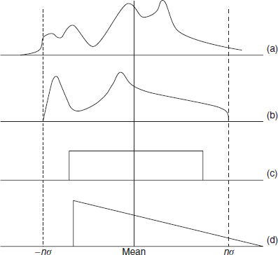
Figure 2.16 Four distributions with the same means and SDs (after W. A. Shewhart).

2.8.2 Effects and Causes

In engineering (and in many other applications) we are really much more concerned with the effects of variation than with the properties and parameters. If, for example, the output of a process varied as in Figure 2.16(c), and the ‘±σ’ lines denoted the allowable tolerance, 100% would be in tolerance. If, however, the process behaved as in (a) or (d), a proportion would be outside tolerance (only at the high end in the case of (d)). Variation can have other effects. A smaller diameter on a shaft might lead to higher oil loss or reduced fatigue life. Higher temperature operation might make an electronic circuit shut down. A higher proportion of fast microprocessors in a production batch would result in higher profit. We must therefore first identify the effects of variation (they are often starkly apparent), and determine whether and to what extent the effects can be reduced. This is not simply a matter of ‘reducing SD’.

The effects of variation can be reduced in two ways:

1. We can compensate for the variation, by methods such as gauging or ‘select on test’ (this curtails the original variation), by providing temperature compensating devices, and so on.
2. We can reduce the variation.

In both cases we must understand the cause, or causes, of the variation. Shewhart categorized manufacturing variation into ‘assignable’ and ‘non-assignable’ causes. (These are also referred to as ‘special causes’ and ‘common causes’.) Assignable variation is any whose cause can be practically and economically identified and reduced: deterministic and functional variation fall into this category. Non-assignable variation is that which remains when all of the assignable variation has been removed. A process in this state is ‘in control’, and will have minimal, random, variation. Note that these are practical criteria, with no strict mathematical basis. Shewhart developed the methods of statistical process control (SPC) around this thinking, with the emphasis on using the data and charting methods to identify and reduce assignable variation, and to keep processes in control. SPC methods are described in detail in Chapter 13.

2.8.3 Tails

People such as life insurance actuaries, clothing manufacturers, and pure scientists are interested in averages and SDs: the behaviour of the bulk of the data. Since most of the sample data, in any situation, will represent this behaviour, they can make credible assertions about these population parameters. However, the further we try to extend the assertions into the tails, the less credible they become, particularly when the assertions are taken beyond any of the data. In engineering we are usually more concerned about the behaviour of variation at the extremes, than that near the average. We are concerned by high stresses, high and low temperatures, slow processors, weak components, and so on. In other words, it is the tails of the distributions that concern us. We often have only small samples to measure or test. Therefore, using conventional mathematical statistics to attempt to understand the nature, causes and effects of variation at the extremes can be misleading. However, these situations can be analysed using the extreme value distributions presented earlier in this chapter.

2.9 Conclusions

These are the aspects that matter in engineering, and they transcend the kind of basic statistical theory that is generally taught and applied. Later teachers, particularly W. E. Deming (see Chapter 1) and Genichi Taguchi (Chapter 11) extended the ideas by demonstrating how reducing variation reduces costs and increases productivity, and by emphasizing the management implications.

Despite all of these reasons why conventional statistical methods can be misleading if used to describe and deal with variation in engineering, they are widely taught and used, and their limitations are hardly considered. Examples are:

• Most textbooks and teaching on SPC emphasise the use of the normal distribution as the basis for charting and decision-making. They emphasize the mathematical aspects, such as probabilities of producing parts outside arbitrary 2σ or 3σ limits, and pay little attention to the practical aspects discussed above.
• Typical design rules for mechanical components in critical stress application conditions, such as aircraft and civil engineering structural components, require that there must be a factor of safety (say 2) between the maximum expected stress and the lower σ value of the expected strength. This approach is really quite arbitrary, and oversimplifies the true nature of variations such as strength and loads, as described above. Why, for example, select 3σ? If the strength of the component were truly normally distributed, about 0.1% of components would be weaker than the 3-σ value. If few components are made and used, the probability of one failing would be very low. However, if many are made and used, the probability of a failure among the larger population would increase proportionately. If the component is used in a very critical application, such as an aircraft engine suspension bolt, this probability might be considered too high to be tolerable. Of course there are often other factors that must be considered, such as weight, cost, and the consequences of failure. The criteria applied to design of a domestic machine might sensibly be less conservative than for a commercial aircraft application.
• The ‘six sigma’ approach to achieving high quality is based on the idea that, if any process is controlled in such a way that only operations that exceed plus or minus 6σ of the underlying distribution will be unacceptable, then fewer than 3.4 per million operations will fail. The exact quantity is based on arbitrary and generally unrealistic assumptions about the distribution functions, as described above. (The ‘six sigma’ approach entails other features, such as the use of a wide range of statistical and other methods to identify and reduce variations of all kinds, and the training and deployment of specialists. It is described in Chapter 17.)

2.10 Discrete Variation

2.10.1 The Binomial Distribution

The binomial distribution describes a situation in which there are only two outcomes, such as pass or fail, and the probability remains the same for all trials. (Trials which give such results are called Bernoulli trials.) Therefore, it is obviously very useful in QA and reliability work. The pdf for the binomial distribution is

This is the probability of obtaining x good items and (n – x) bad items, in a sample of n items, when the probability of selecting a good item is p and of selecting a bad item is q. The mean of the binomial distribution (from Eq. 2.13) is given by

and the SD from (Eq. 2.17)

The binomial distribution can only have values at points where x is an integer. The cdf of the binomial distribution (i.e. the probability of obtaining r or fewer successes in n trials) is given by

Excel functions for the binomial distribution are: pdf f(x) =BINOMDIST(x, n, p, FALSE) and cdf F(r) =BINOMDIST(r, n, p, TRUE).

Example 2.6

A frequent application of the cumulative binomial distribution is in quality control acceptance sampling. For example, if the acceptance criterion for a production line is that not more than 4 defectives may be found in a sample of 20, we can determine the probability of acceptance of a lot if the production process yields 10% defectives.

From Eq. (2.40),

Utilising Excel spreadsheet F(4) = BINOMDIST(4, 20, 0.1, TRUE) = 0.9568.

Example 2.7

An aircraft landing gear has 4 tyres. Experience shows that tyre bursts occur on average on 1 landing in 1200. Assuming that tyre bursts occur independently of one another, and that a safe landing can be made if not more than 2 tyres burst, what is the probability of an unsafe landing?

If n is the number of tyres and p is the probability of a tyre bursting,

The probability of a safe landing is the probability that not more than 2 tyres burst.

Again, utilizing Excel function: F(2) = BINOMDIST(2, 4, 0.000 83, TRUE) = 0.999 999 997 714 Therefore the probability of an unsafe landing is

2.10.2 The Poisson Distribution

If events are Poisson-distributed they occur at a constant average rate, with only one of the two outcomes countable, for example, the number of failures in a given time or defects in a length of wire:

where μ is the mean rate of occurrence. Excel functions for the Poisson distribution are: pdf f(x) = POISSON(x, MEAN, FALSE) and cdf = POISSON(x, MEAN, TRUE). In this case, MEAN = μ × Duration (in time, length, etc.)

For example, if we need to know the probability of not more than 3 failures occurring in 1000 h of operation of a system, when the mean rate of failures is 1 per 1000 h, (μ = 1/1000, x = 3) we can calculate the MEAN = μ × 1000 h = 1.0.

Therefore P(x ≤ 3) = POISSON(3, 1, TRUE) = 0.981.

The Poisson distribution can also be considered as an extension of the binomial distribution, in which n is considered infinite or very large. Therefore it gives a good approximation to the binomial distribution, when p or q are small and n is large. This is useful in sampling work where the proportion of defectives is low (i.e. p < 0.1).

The Poisson approximation is

This approximation allows us to use Poisson tables or charts in appropriate cases and also simplifies calculations. However the applications of Poisson approximation became somewhat limited after computerized applications, such as Excel and various statistical programs became available.

It is also important to note, that if times to failure are exponentially distributed (see exponential distribution earlier this chapter), the probability of x failures is Poisson-distributed. For example, if the MTBF is 100 h, the probability of having more than 15 failures in 1000 h is derived as:

Probability of having 15 failures or less can be calculated using the Poisson Excel formula POISSON (15,10,TRUE) = 0.9513. Thus the probability of having more than 15 failures is 1 – 0.9513 = 0.0487.

Example 2.8

If the probability of an item failing is 0.001, what is the probability of 3 failing out of a population of 2000?

The binomial solution is

utilizing Excel: BINOMDIST(3, 2000, 0.001, FALSE) = 0.180 53.

As an alternative, the Poisson approximation can be applied. The Poisson approximation is evaluated as follows:

As the normal distribution represents a limiting case of the binomial and Poisson distributions, it can be used to provide a good approximation to these distributions. For example, it can be used when 0.1 > p > 0.9 and n is large.

Then

Example 2.9

What is the probability of having not more than 20 failures if n = 100, p = 0.14?

Using the binomial distribution,

Using the normal approximation

Referring to Appendix 1, P₂₀ = 0.9582 or Excel: = NORMSDIST(1.73) = 0.958 18.

As p → 0.5, the approximation improves, and we can then use it with smaller values of n. Typically, if p = 0.4, we can use the approximation with n = 50.

2.11 Statistical Confidence

Earlier in this chapter we mentioned the problem of statistical confidence. Confidence is the exact fraction of times the confidence interval will include the true value, if the experiment is repeated many times. The confidence interval is the interval between the upper and lower confidence limits. Confidence intervals are used in making an assertion about a population given data from a sample. Clearly, the larger the sample the greater will be our intuitive confidence that the estimate of the population parameter will be close to the true value. To illustrate this point, let's use the hypothetical example where we test 10 samples out of large population and 1 sample fails with 9 surviving. In this case we may infer a non-parametric reliability of 90%. If we test 100 samples from the same population and experience 10 failures, we may again similarly infer 90% reliability. However our confidence in that number will be much higher than that in the first case due to the larger sample in the second case.

Statistical confidence and engineering confidence must not be confused; statistical confidence takes no account of engineering or process knowledge or changes which might make sample data unrepresentative. Derived statistical confidence values must always be interpreted in the light of engineering knowledge, which might serve to increase or decrease our engineering confidence.

2.11.1 Confidence Limits on Continuous Variables

If the population value x follows a normal distribution, it can be shown that the means, , of samples drawn from it are also normally distributed, with variance σ²/n (SD = σ/n^1/2). The SD of the sample means is also called the standard error of the estimate, and is denoted S_x.

If x is not normally distributed, provided that n is large (> 30), will tend to a normal distribution. If the distribution of x is not excessively skewed (and is unimodal) the normal approximation for at values of n as small as 6 or 7 may be acceptable.

These results are derived from the central limit theorem, mentioned in Section 2.6.1. They are of great value in deriving confidence limits on population parameters, based on sample data. In reliability work it is not usually necessary to derive exact confidence limits and therefore the approximate methods described are quite adequate.

Example 2.10

A sample of 100 values has a mean of 27.56, with a standard deviation of 1.10. Derive 95% confidence limits for the population mean. (Assume that the sample means are normally distributed.)

In this case, the SD of the sample means, or standard error of the estimate, is

We can refer to the table of the normal cdf (Appendix 1) to obtain the 95% single-sided confidence limits. The closest tabulated value of z is 1.65.

Alternatively we can run Excel's Tools – Goal Seek for Z in NORMSDIST(Z) = 0.95 (see Figure 2.17) to calculate the Z-value approaching 1.65.

Therefore, approximately ±1.65 SDs are enclosed within the 95% single-sided confidence limits. Since the normal distribution is symmetrical, the 90% double-sided confidence interval will exclude 5% of values at either limit.

In the example, 1.65 SDs = 0.18. Therefore the 95% confidence limits on the population mean are 27.56 ± 0.18, and the 90% confidence interval is (27.56 − 0.18) to (27.56 + 0.18).

As a guide in confidence calculations, assuming a normal distribution see Figure 2.18:

± 1.65 SDs enclose approximately 90% confidence limits (i.e. 5% lie in each tail).

± 2.0 SDs enclose approximately 95% confidence limits (i.e. 2.5% lie in each tail).

± 2.5 SDs enclose approximately 99% confidence limits (i.e. 0.5% lie in each tail).

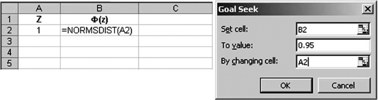
Figure 2.17 Utilizing Excel's Goal Seek to find Z-value corresponding to the 95% confidence interval.

Figure 2.18 Confidence levels for normal distribution.

2.12 Statistical Hypothesis Testing

It is often necessary to determine whether observed differences between the statistics of a sample and prior knowledge of a population, or between two sets of sample statistics, are statistically significant or due merely to chance. The variation inherent in sampling makes this distinction itself subject to chance. We need, therefore, to have methods for carrying out such tests. Statistical hypothesis testing is similar to confidence estimation, but instead of asking the question How confident are we that the population parameter value is within the given limits? (On the assumption that the sample and the population come from the same distribution), we ask How significant is the deviation of the sample?

In statistical hypothesis testing, we set up a null hypothesis, that is, that the two sets of information are derived from the same distribution. We then derive the significance to which this inference is tenable. As in confidence estimation, the significance we can attach to the inference will depend upon the size of the sample. Many significance test techniques have been developed for dealing with the many types of situation which can be encountered.

In this section we will cover a few of the simpler methods commonly used in reliability work. However, the reader should be aware that the methods described and the more advanced techniques are readily accessible on modern calculators and as computer programs. The texts listed in the Bibliography should be used to identify appropriate tests and tables for special cases.

2.12.1 Tests for Differences in Means (z Test)

A very common significance test is for the hypothesis that the mean of a set of data is the same as that of an assumed normal population, with known μ and σ. This is the z test. The z-statistic is given by

where n is the sample size, μ the population mean, the sample mean and σ the population SD. We then derive the significance level from the normal cdf table.

Example 2.11

A type of roller bearing has a time to failure which is normally distributed, with a mean of 6000h and an SD of 450h. A sample of nine, using a changed lubricant, gave a mean life of 6400h. Has the new lubricant resulted in a statistically significant change in mean life?

From Appendix 1, z = 2.67 indicates a cumulative probability of 0.996. This indicates that there is only 0.004 probability of observing this change purely by chance, that is, the change is significant at the 0.4% level. Thus we reject the null hypothesis that the sample data are derived from the same normal distribution as the population, and infer that the new lubricant does provide an increased life.

Significance is denoted by α. In engineering, a significance level of less than 5% can usually be considered to be sufficient evidence upon which to reject a null hypothesis. A significance of greater than 10% would not normally constitute sufficient evidence, and we might either reject the null hypothesis or perform further trials to obtain more data. The significance level considered sufficient will depend upon the importance of the decision to be made based on the evidence. As with confidence, significance should also be assessed in the light of engineering knowledge.

Instead of testing a sample against a population, we may need to determine whether there is a statistically significant difference between the means of two samples. The SD of the distribution of the difference in the means of the samples is

The SD of the distribution of the difference of the sampling means is called the standard error of the difference. This test assumes that the SDs are the population SDs. Then

Example 2.12

In Example 2.11, if the mean value of 6000 and SD of 450 were in fact derived from a sample of 60, does the mean of 6400, with an SD of 380 from a sample of 9 represent a statistically significant difference?

The difference in the means is

6400 – 6000 = 400

The standard error of the difference is

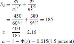
We can therefore say that the difference is highly significant, a similar result to that of Example 2.11.

2.12.2 Use of the z Test for Binomial Trials

We can also use the z test for testing the significance of binomial data. Since in such cases we are concerned with both extremes of the distribution, we use a two-sided test, that is, we use 2α instead of α.

Example 2.13

Two sets of tests give the results in Table 2.2. We need to know if the differences in test results are statistically significant.

The null hypothesis that the tests are without difference is examined by combining the test results:

The standard error of the difference in proportions is

Table 2.2 Results for tests in Example 2.13.

The proportion failed in test 1 is 16/217 = 0.074. The proportion failed in test 2 is 14/310 = 0.045. The difference in proportions is 0.074 – 0.045 = 0.029. Therefore z = 0.029/0.020 = 1.45, giving

With such a result, we would be unable to reject the null hypothesis and would therefore infer that the difference between the tests is not very significant.

2.12.3 χ² Test for Significance

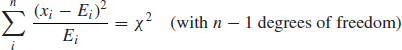
The χ² test for the significance of differences is used when we can make no assumptions about the underlying distributions. The value of the χ² statistic is calculated by summing the terms

where x_i and E_i are the ith observed and expected values, respectively. This value is compared with the χ² value appropriate to the required significance level.

Example 2.14

Using the data of Example 2.13, the χ² test is set up as follows:

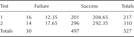
The first number in each column is the observed value and the second number is the expected value based upon the totals of the observations (e.g. expected failures in test 1 = 30/527 × 217 = 12.35).

The number of DF is one less than the number of different possibilities which could exist. In this case there is only one DF, since there are two possibilities – pass and fail. The value of χ² of 1.94 for 1 DF (from Appendix 2) occurs between 0.1 and 0.2 (alternatively, CHIDIST(1.94, 1) = 0.1636). Therefore a cumulative probability is between 80 and 90% (1- CHIDIST(1.94, 1) = 0.8363). The difference between the observed data sets is therefore not significant. This inference is the same as that derived in Example 2.13.

2.12.4 Tests for Differences in Variances. Variance Ratio Test (F Test)

The significance tests for differences in means described above have been based on the assumption in the null hypothesis that the samples came from the same normal distribution, and therefore should have a common mean. We can also perform significance tests on the differences of variances. The variance ratio, F, is defined as

Table 2.3 Life test data on two items.

Values of the F distribution are well tabulated against the number of degrees of freedom in the two variance estimates (for a sample size n, DF = n − 1) and can easily be found on the Internet (see for example NIST, 2011).

The Excel¯ function for the values of F-distribution is FINV(P, DF1, DF2). Where P is a probability (significance level), DF1 is degrees of freedom for the first population (numerator) and DF2 for the second population (denominator). When the value of F-distribution and degrees of freedom are known, the probability can be calculated using the other Excel function FDIST(F, DF1, DF2). The use of the F test is illustrated by Example 2.15.

Example 2.15

Life test data on two items give the results in Table 2.3.

Entering the tables of F values at 19 DF for the greater variance estimate and 9 DF for the lesser variance estimate, we see that at the 5% level our value for F is less than the tabulated value. Therefore the difference in the variances is not significant at the 5% level. The Excel solution would involve the Goal Seek function (similar to the example in Figure 2.17) for the value P as FINF(P, 19, 9) = 1.42 and would produce P = 0.3, which is much higher than the required 5% risk level.

2.13 Non-Parametric Inferential Methods

Methods have been developed for measuring and comparing statistical variables when no assumption is made as to the form of the underlying distributions. These are called non-parametric (or distribution-free) statistical methods. They are only slightly less powerful than parametric methods in terms of the accuracy of the inferences derived for assumed normal distributions. However, they are more powerful when the distributions are not normal. They are also simple to use. Therefore they can be very useful in reliability work provided that the data being analysed are independently and identically distributed (IID). The implications of data not independently and identically distributed are covered in Section 2.15 and in the next chapter.

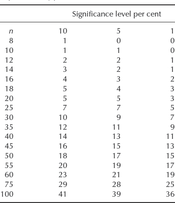
Table 2.4 Critical values of r for the sign test. Reproduced by permission of McGraw-Hill.

2.13.1 Comparison of Median Values

2.13.1.1 The Sign Test

If a null hypothesis states that the median values of two samples are the same, then about half the values of each sample should lie on either side of the median. Therefore about half the values of (x_i – ) should be positive and half negative. If the null hypothesis is true and r is the number of differences with one sign, then r has a binomial distribution with parameters n and p = 1/2. We can therefore use the binomial distribution to determine critical values of r to test whether there is a statistically significant difference between the median values. Table 2.4 gives critical values for r for the sign test where r is the number of less frequent signs. If the value of r is equal to or less than the tabulated value the null hypothesis is rejected.

Example 2.16

Ten items are tested to failure, with lives

98, 125, 141, 72, 119, 88, 64, 187, 92, 114

Do these results indicate a statistically significant change from the previous median life of 125? The sign test result is

−0+ -----+--

that is, r = 2, n = 9 (since one difference = 0, we discard this item).

Table 2.4 shows that r is greater than the critical value for n = 9 at the 10% significance level, and therefore the difference in median values is not statistically significant at this level.

2.13.1.2 The Weighted Sign Test

We can use the sign test to determine the likely magnitude of differences between samples when differences in medians are significant. The amount by which the samples are believed to differ are added to (or subtracted from) the values of one of the samples, and the sign test is then performed as described above. The test then indicates whether the two samples differ significantly by the weighted value.

2.13.1.3 Tests for Variance

Non-parametric tests for analysis of variance are given in Chapter 11.

2.13.1.4 Reliability Estimates

Non-parametric methods for estimating reliability values are given in Chapter 13.

2.14 Goodness of Fit

In analysing statistical data we need to determine how well the data fit an assumed distribution. The goodness of fit can be tested statistically, to provide a level of significance that the null hypothesis (i.e. that the data do fit the assumed distribution) is rejected. Goodness-of-fit testing is an extension of significance testing in which the sample cdf is compared with the assumed true cdf.

A number of methods are available to test how closely a set of data fits an assumed distribution. As with significance testing, the power of these tests in rejecting incorrect hypotheses varies with the number and type of data available, and with the assumption being tested.

2.14.1 The χ² Goodness-of-Fit Test

A commonly used and versatile test is the χ² goodness-of-fit test, since it is equally applicable to any assumed distribution, provided that a reasonably large number of data points is available. For accuracy, it is desirable to have at least three data classes, or cells, with at least five data points in each cell.

The justification for the χ² goodness-of-fit test is the assumption that, if a sample is divided into n cells (i.e. we have ν degrees of freedom where ν = n −1), then the values within each cell would be normally distributed about the expected value, if the assumed distribution is correct, that is, if x_i and E_i are the observed and expected values for cell i:

High values of χ² cast doubt on the null hypothesis. The null hypothesis is usually rejected when the value of χ² falls outside the 90th percentile. If χ² is below this value, there is insufficient information to reject the hypothesis that the data come from the supposed distribution. If we obtain a very low χ² (e.g. less than the 10th percentile), it suggests that the data correspond more closely to the supposed distribution than natural sampling variability would allow (i.e. perhaps the data have been ‘doctored’ in some way).

Table 2.5 Data from an overstress life test of transistors.

The application can be described by use of an example.

Example 2.17

Failure data of transistors are given in Table 2.5. What is the likelihood that failures occur at a constant average rate of 12 failures/1000 hours?

Referring to Appendix 2 for values of χ² with χ² with (n − 1) = 4 degrees of freedom, 6.67 lies between the 80th and 90th percentiles of the χ² distribution (risk factors between 0.1 and 0.2). CHIDIST (6.67, 4) = 0.1543. Therefore the null hypothesis that the data are derived from a constant hazard rate process cannot be rejected at the 90% level (risk factor needs to be less than 0.1).

If an assumed distribution gave expected values of 20, 15, 12, 10, 9 (i.e. a decreasing hazard rate), then

χ² = 1.11 lies close to the 10th percentile (CHIDIST(1.11, 4) = 0.8926). Therefore we cannot reject the null hypothesis of the decreasing hazard rate distribution at the 90% level.

Note that the E_i values should always be at least 5. Cells should be amalgamated if necessary to achieve this, with the degrees of freedom reduced accordingly. Also, if we have estimated the parameters of the distribution we are fitting to, the degrees of freedom should be reduced by the number of parameters estimated.

2.14.2 The Kolmogorov–Smirnov Test

Another goodness-of-fit test commonly used in reliability work is the Kolmogorov–Smirnov (K–S) test. It is rather simpler to use than the χ² test and can give better results with small numbers of data points. It is also convenient to use in conjunction with probability plots (see Chapter 3), since it is based upon cumulative ranked data, that is, the sample cdf. The procedure is:

1. Tabulate the ranked failure data. Calculate the values of |x_i – E_i| where x_i is the ith cumulative rank value and E_i the expected cumulative rank value for the assumed distribution.
2. Determine the highest single value.
3. Compare this value with the appropriate K–S value (Appendix 3).

Table 2.6 Failure data with ranked values of x_i.

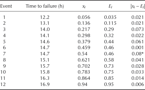
Example 2.18

Table 2.6 shows failure data with the ranked values of x_i. We wish to test the null hypothesis that the data do not fit a normal distribution with parameters which give the tabulated cumulative values of E_i. Therefore, in the E_i column we list the expected value of proportion failed at each failure time.

The largest value of |x_i – E_i| is 0.08 (shown in Table 2.6 by*). The Kolmogorov–Smirnov table (Appendix 3) shows that, for n = 12, the critical value of |x_i – E_i| is 0.338 at the 10% significance level. Therefore the null hypothesis is not rejected at this level, and we can accept the data as coming from the hypothesized normal distribution.

Example 2.18 shows quite a large difference between the critical K–S value and the largest value of |x_i – E_i|. When the parameters of the assumed cdf are being estimated from the sample data, as in this example, the critical K–S values are too large and give lower significance levels than are appropriate in the circumstances. In order to correct for this, the critical values should be multiplied by the factors:

where β is the Weibull shape parameter. Therefore, in Example 2.18, since the Weibull β value appropriate to the normal distribution is > 3.0, the corrected K–S critical value is 0.338 × 0.70 = 0.237.

2.15 Series of Events (Point Processes)

Situations in which discrete events occur randomly in a continuum (e.g. time) cannot be truly represented by a single continuous distribution function. Failures occurring in repairable systems, aircraft accidents and vehicle traffic flow past a point are examples of series of discrete events. These situations are called stochastic point processes. They can be analysed using the statistics of event series.

The Poisson distribution function (Eq. 2.41) describes the situation in which events occur randomly and at a constant average rate. This situation is described by a homogeneous Poisson process (HPP). A HPP is a stationary point process, since the distribution of the number of events in an interval of fixed length does not vary, regardless of when (where) the interval is sampled.

The Poisson distribution function is (from (2.41))

where λ is the mean rate of occurrence, so that λx is the expected number of events in (0, x).

In a non-homogeneous Poisson process (NHPP) the point process is non-stationary (rate of occurrence is a function of time), so that the distribution of the number of events in an interval of fixed length changes as x increases. Typically, the discrete events (e.g. failures) might occur at an increasing or decreasing rate.

Note that an essential condition of any homogeneous Poisson process is that the probabilities of events occurring in any period are independent of what has occurred in preceding periods. A HPP describes a sequence of independently and identically exponentially distributed (IIED) random variables. A NHPP describes a sequence of random variables which is neither independently nor identically distributed.

2.15.1 Trend Analysis (Time Series Analysis)

When analysing data from a stochastic point process it is important to determine whether the process has a trend, that is, to know whether a failure rate is increasing, decreasing or constant. We can test for trends by analysing the arrival values of the event series. The arrival values x₁, x₂, . . ., x_n are the values of the independent variables (e.g. time) from x = 0 at which each event occurs. The interarrival values X₁, X₂, . . .X_n are the intervals between successive events 1, 2, . . ., n, from x = 0. Figure 2.19 shows the distinction between arrival and interarrival values.

If x₀ is the period of observation, then the test statistic for trend is

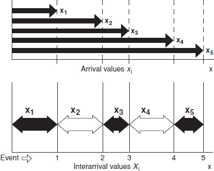
Figure 2.19 Arrival and interarrival values.

This is called the centroid test or the Laplace test. It compares the centroid of the observed arrival values with the mid-point of the period of observation. If U = 0 there is no trend, that is, the process is stationary. If U < 0 the trend is decreasing, that is, the interarrival values are tending to become larger. Conversely, when U > 0 the trend is increasing, that is, interarrival values are tending to become progressively smaller.

If the period of observation ends at an event, use (n − 1) instead of n and exclude the time to the last event from the summation Σx_i.

We can test the null hypothesis that there is no trend in the chronologically ordered data by testing the value of U against the values of the standard normal variate, z. For example, using Appendix 1 or Excel function, if U = 1.65, for z = 1.65, Φ(z) = 0.95. Therefore we can reject the null hypothesis at the 5% significance level.

The centroid test is theoretically adequate if n ≥ 4, when the observation interval ends with an event, and if n ≥ 3, when the interval is terminated at a predetermined time.

The method is also called time series analysis (TSA).

Example 2.19

Arrival values (x_i) and interarrival values (X_i) between 12 successive failures of a component are as follows (observation ends at the last failure):

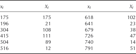
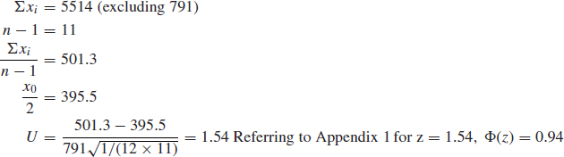
Therefore we can reject the null hypothesis that there is no trend at the 6% significance level. The interarrival times are becoming shorter, that is, the failure rate is increasing.

The existence of a trend in the data, as in Example 2.19, indicates that the interarrival values are not independently and identically distributed (IID). This is a very important point to consider in the analysis of failure data, as will be explained in Chapter 13.

2.15.2 Superimposed Processes

If a number of separate stochastic point process combine to form an overall process, for example, failure processes of individual components (or sockets) in a system, these are called superimposed processes. If the individual random variables are IID exponential then the overall process variable is also IID exponential and the process is HPP.

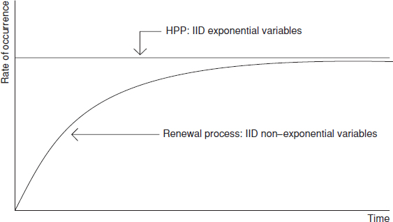
Figure 2.20 Rate of occurrence for superimposed processes.

If the individual variables are IID non-exponential, the overall process will tend to a HPP. Such a process is called a renewal process or ordinary renewal process (ORD). Figure 2.20 shows these processes. Renewal process analytics is often applied to describe the behaviour of a repairable system, where initial failures follow an exponential or any other statistical distribution and failed parts can be repaired to “as good as new” condition, returned to operation and experience secondary failures. None of the traditional statistical distribution covered in this chapter can be applied due to the fact that the failed units are not taken out of the total population, therefore the cdf can theoretically be greater than 1.0 in the cases where the total number of failures exceeds the size of the population. The renewal process can be described by the fundamental renewal equation:

Where Λ(t) is the renewal function, which would represent the number of replacements (repairs) per unit and F(t) is the cdf of the primary failures (as if there were no replacement of the failed parts).

2.16 Computer Software for Statistics

Computer software is available which can be used to carry out the analytical techniques described in this chapter and in later chapters which describe particular applications. As mentioned before, Microsoft Excel has a wide variety of statistical functions, covering most of the equations presented in this chapter. Among the software packages specializing in statistical analysis Minitab¯ statistical software and SAS¯ are probably most widely used around the world. Minitab is a comprehensive statistical package covering various aspects of data analysis, quality, design of experiments, and other engineering and non-engineering applications. SAS has more emphasis on business applications.

2.17 Practical Conclusions

Whilst the mathematical methods described in this chapter can be useful for providing insights and for forecasting, it is important that their limitations are appreciated. They are mathematical models, and they do not necessarily reflect reality in the way that deterministic, physics-based formulae do. The important points that must be borne in mind when applying statistical methods to engineering are:

• Real variation is seldom normal.
• The most important variation, as far as reliability is concerned, is usually that in the tails, where there is inevitably less (or no) data, the data are more uncertain, and where conventional statistical models can be most misleading.
• Variation can change over time, so that the patterns measured at one time might not represent the true situation at another. We will cover this aspect in more detail in later chapters.
• There might be interaction effects between variables, causing combined effects that are more significant than those of individual variations. This aspect will be covered in the later chapters.
• Variation in engineering is usually made or influenced by people. People do not behave in accordance with any credible mathematical models.
• Most engineering education in statistics covers only the mathematics, and few statisticians understand the practical aspects of the engineering problems they help to solve. This leads to inappropriate analyses and conclusions, and to a distrust of statistical methods among engineers.

We must strike an appropriate balance between using deterministic and statistical methods. For example, if we conduct a test in which an item is released from a height, and if it drops the test is a success, with results as follows:

items tested (0 failures): 0 1 10 20

then we could infer that the 80% confidence that the reliability is at least 0.9 would be:

0 0.90 0.98 0.99

This assumes that the data are entirely statistical, that is, we have no prior knowledge of the physics or engineering. On the other hand, if we are confident that we have such knowledge (in this case, that the force of gravity will always act on the released items), then we will have 100% confidence in 100% reliability, even without performing any tests. In such deterministic cases statistical tests and interpretations are inappropriate.

However, many engineering situations can range from deterministic to statistical. For example, there might be cases when the release mechanism fails to open properly. The causes and effects of variations are often uncertain (particularly when interactions exist), so we must make the best use of our knowledge and use the best methods to explore the uncertainties.

Statistical tests can, by themselves, generate misleading results. We have discussed this in the context of extrapolations beyond the range of measured data. Another example might be a series of tests that indicate that an item operated at high stress is more reliable than when operated at low stress. The results might be due to the items on the high-stress tests being manufactured using a better process, or the high stress may actually improve the reliability (e.g. a higher temperature might improve the performance of a seal), or the results might be due to chance and unrepresentative of future tests. The cause of the observed reliability difference must be ascertained and understood in engineering terms. Sometimes this can be difficult.

Ultimately, all of our understanding should be based upon real knowledge (scientific, human, etc.). The statistical methods can provide clues to help us to gain such knowledge. The quotation from Kendall and Stuart on the inside of the front cover should be the motto for all statistics applications.

Questions

1. In the test firing of a missile, there are some events that are known to cause the missile to fail to reach its target. These events are listed below; together with their approximate probabilities of occurrence during a flight:

   Event	Probability
   (A1) Cloud reflection	0.0001
   (A2) Precipitation	0.005
   (A3) Target evasion	0.002
   (A4) Electronic countermeasures	0.04

   The probabilities of failure if these events occur are:

   

   Use Bayes' theorem (Eq. 2.10) to calculate the probability of each of these events being the cause in the event of a missile failing to reach its target.

2. For a device with a failure probability of 0.02 when subjected to a specific test environment, use the binomial distribution to calculate the probabilities that a test sample of 25 devices will contain (a) no failures; (b) one failure; (c) more than one failure.
3. Repeat question 2 for a failure probability of 0.2.
4. Repeat questions 2 and 3 using the Poisson approximation to the binomial, and comment on the answers.
5. One of your suppliers has belatedly realized that about 10% of the batches of a particular component recently supplied to you have a manufacturing fault that has reduced their reliability. There is no external or visual means of identifying these substandard components. Batch identity has, however, been maintained, so your problem is to sort batches that have this fault (‘bad’ batches) from the rest (‘good’ batches). An accelerated test has been devised such that components from good batches have a failure probability of 0.02 whereas those from bad batches have a failure probability of 0.2. A sampling plan has been devised as follows:
   1. Take a random sample of 25 items from each unknown batch, and subject them to the test.
   2. If there are 0 or 1 failed components, decide that the batch is a good one.
   3. If there are two or more failures, decide that the batch is a bad one.

   There are risks in this procedure. In particular, there are (i) the risk of deciding that a good batch is bad; and (ii) the risk of deciding that a bad batch is good. Use Bayes' theorem and your answers to questions 2 and 3 to evaluate these risks.

6. 1. Explain the circumstances in which you would expect observed failure times to conform to an exponential distribution.
   2. Explain the relationship between the exponential and Poisson distributions in a reliability context.
   3. For equipment with an MTBF of 350 h calculate the probability of surviving a 200 h mission without failure.
7. A railway train is fitted with three engine/transmission units that can be assumed to exhibit a constant hazard with a mean life of 200 h. In a 15 h working day, calculate the probability of a train having: (a) no failed engine/transmission units, (b) not more than one failed unit, (c) not more than two failed units.
8. Assuming the exponential failure distribution, calculate the probability of a system surviving an operation time equal to twice the duration of the MTBF.
9. 1. Explain, using sketches where necessary, the meanings of the following terms used in describing the reliability behaviour of components; and show clearly how they are related to each other: (i) lifetime probability density function; (ii) cumulative distribution function; (iii) reliability function; (iv) hazard function.
   2. Write down the expression for the cumulative distribution function (cdf) of the two-parameter Weibull distribution. Define its parameters and produce sketches to show how changing their values influences the cdf and the hazard function.
10. Ten components were tested to failure. The ordered ages at failure (hours) were: 70.9; 87.2; 101.7; 104.2; 106.2; 111.4; 112.6; 116.7; 143.0; 150.9.
    1. On the assumption that these times to failure are normally distributed, estimate the component reliability and the hazard function (i) at age 100 h; and (ii) at age 150 h.
    2. Use a Kolmogorov–Smirnov test to see whether it is reasonable to assume normality.
11. A flywheel is retained on a shaft by five bolts, which are each tightened to a specified torque of 50 ± 5 Nm. A sample of 20 assemblies was checked for bolt torque. The results from the 100 bolts had a mean of 47.2 Nm and a standard deviation of 1.38 Nm.
    1. Assuming that torques are normally distributed, estimate the proportion below 45 Nm.
    2. For a given assembly, what is the probability of (i) there being no bolts below 45 Nm; (ii) there being at least one bolt below 45 Nm; (iii) there being fewer than two bolts above 45 Nm; (iv) all five bolts being below 45 Nm.
    3. In the overall sample of 100 bolts, four were actually found with torques below 45 Nm. (i) Comment on the comparison between this result and your answer to (a) above. (ii) Use this result to obtain a 90% two-sided confidence interval for the proportion below 45 Nm.
    4. Explain the meaning of the confidence interval in c (ii) above as you would to an intelligent, but non-technically-minded, manager.
    5. The lowest torque bolt in each assembly was identified. For these 20 bolts, the mean torque was 45.5 Nm and the standard deviation 0.88 Nm. Assuming an appropriate extreme-value distribution, calculate the probability that on a given assembly the lowest torque will be (i) below 45 Nm; (ii) below 44 Nm.
12. The following data are the times (hours) between successive failures in a machining centre: 96; 81; 105; 34; 92; 81; 89; 138; 75; 156; 205; 111; 177.

    Calculate the trend statistic (Eq. 2.46) and test its significance.

13. Describe four ways in which the variation of an engineering parameter might be different from that based upon assuming that the normal distribution function is the correct model. Give an example in each case.
14. In most statistical applications the results that matter most relate to the behaviour of the majority of the population being studied. Why is this not the case in most engineering applications?
15. Ten items are put on test, until all have failed. The first failure occurs at 35 000 operating cycles. Regression analysis of the times to failure shows a good fit to a two-parameter Weibull distribution, and the distribution parameters are derived. The specification states that the item should have a B₁₀ life of 30 000 cycles. Discuss the practical implications assuming that the test shows compliance with the specification.
16. In question 15, how might your judgment be influenced if the item is:
    1. A steel bolt subject to fatigue loading?
    2. A plastic component in a child's toy?
    3. A lighting unit?
    4. A bearing in a gearbox?
    5. A light-emitting diode?

    (You might like to try this question after studying Chapters 8 and 9.)

17. Explain what is meant by ‘statistical confidence’. How might statistical confidence derived from an experiment be modified in the light of engineering knowledge?
18. In Example 2.7 describe three factors that could invalidate the assumption that tyre failures occur independently of one another. In what ways might the assumption be more valid for car tyres?
19. What is the probability of having not more than 20 but not less than 10 failures if n = 100, p = 0.14 (Section 2.10)?
    1. Using the binomial distribution
    2. Using the normal approximation
20. The life of an electronic controller is distributed lognormally, with the parameters μ = 20 and σ = 10. What is the probability that a controller will last (a) at least 50 h? (b) at least 200 h?
21. A commercial washing machine has a non-repairable motor with a constant failure rate of 0.08 failure per year. The service organization has purchased two spare motors. If the design life of the washing machine is 7 years, what is the probability that two spares will be adequate. Hint: assume Poisson distribution.
22. Compare reliability values for the two products, Product A with exponentially distributed life and product B with Weibull distributed life. The parameters are MTBF_A = η_B = 1000 h. Compare the reliabilities at 300 hours for:

    β_B = 0.5

    β_B = 1.0

    β_B = 3.0

    How would you describe the effect of the Weibull shape parameter β on the reliability if the scale parameter remains the same?

23. Show the derivations of the hazard rate and cumulative hazard function for the Weibull distribution
24. Calculate the cumulative hazard rate for the Weibull distribution with the parameters β = 2.5 η = 200 h at time t = 100 h.

Bibliography

Helpful introductory sources

Chatfield, C. (1983) Statistics for Technology, 2nd edn, Chapman & Hall.

Conover, W. (1998) Practical Non-parametric Statistics, J. Wiley.

Hines, W. and Montgomery, D. (1990) Probability and Statistics in Engineering and Management Science, 3rd edn, Wiley.

Langley, R. (1979) Practical Statistics Simply Explained, 2nd edn, Pan.

Modarres, M. Kaminskiy, M. Krivtsov V. (1999) Reliability Engineering and Risk Analysis, 2nd edn, Marcel Dekker.

Montgomery, D., Runger, G., Hubele, M. (2006) Engineering Statistics, 4th edn, J. Wiley.

NIST (2011) Section 1.3.6.7.3 Upper Critical Values of the F Distribution. Engineering Statistics Handbook, published by NIST. Available at: http://www.itl.nist.gov/div898/handbook/eda/section3/eda3673.htm.

Ryan, T. (2000) Statistical Methods for Quality Improvement, Wiley.

More advanced works

Abernethy, R. (2003) The New Weibull Handbook, 5th edn, Dr. Robert Abernethy.

Duncan, A. (1986) Quality Control and Industrial Statistics, 5th edn, Irwin.

Hahn G., Meeker, W. (1991) Statistical Intervals, a Guide for Practitioners, J. Wiley.

Hollander, M., Wolfe, D. (1999) Non-parametric Statistical Methods, 2nd edn, J. Wiley.

Kleyner, A., Bhagath, S., Gasparini, M. et al. (1997) Bayesian techniques to reduce the sample size in automotive electronics attribute testing. Microelectronics and Reliability, 37(6), 879–883.

Martz, H. and Waller, A. (1982) Bayesian Reliability Analysis, J. Wiley.

Modarres, M., Kaminskiy, M. and Krivtsov, V. (1999) Reliability Engineering and Risk MINITAB (2011) (General purpose statistics training and application software). Minitab Inc. 3081 Enterprise Drive, PA 16801, USA. (The MINITAB Handbook (Duxbury Press, Boston) is an excellent introduction to basic statistics), www.mintab.com.

National Institute of Standards and Technology (NIST). NIST/SEMATECH e-Handbook of Statistical Methods http://www.itl.nist.gov/div898/handbook/October 2010.

Nelson, W. (2003) Applied Life Data Analysis, J. Wiley.

SAS Business Analytics Software Manual. http://www.sas.com/resources/.

Seitano, S. (2001) Engineering Uncertainty and Risk Analysis, Hydroscience Inc.

Wassreman, G. (2003) Reliability Verification Testing, and Analysis in Engineering Design, Marcel Dekker.