4

Monte Carlo Simulation

4.1 Introduction

Monte Carlo (MC) simulation is a useful tool for modelling phenomena with significant uncertainty in inputs and has a multitude of applications including reliability, availability and logistics forecasting, risk analysis, load-strength interference analysis (Chapter 5), random processes simulation including repairable systems (Chapter 13), probabilistic design, uncertainty propagation, geometric dimensioning and tolerancing, and a variety of business applications.

The concept of the Monte Carlo method comes from the gaming tables at the casinos of Monte Carlo. It is a class of probabilistic computational algorithms that rely on repeated sampling of random variables of interest to compute the results.

Simplistic simulation can be done with spreadsheet software, while more sophisticated modelling can be done with the use of software packages, like Palisade @Risk¯, Minitab¯, Crystal Ball¯ and many others.

4.2 Monte Carlo Simulation Basics

Monte Carlo simulation can be defined as a method for iteratively evaluating a deterministic model using sets of random numbers as inputs. It is a fairly simple mathematical procedure, with random inputs and random outputs: γ = f(x₁, x₂, . . ., x_n), where the input values are sampled and the output values are recorded and analysed as illustrated in Figure 4.1.

In order to run Monte Carlo simulation we need to generate random variables that follow an arbitrary statistical distribution. The inputs are randomly generated from probability distributions to simulate the process of sampling from an actual population, therefore we choose a distribution for each input that best represents our current state of knowledge. The data generated from a simulation can be represented in a basic statistic format, a histogram, fitted into a probability distribution function, or any other format needed for the analysis.

4.3 Additional Statistical Distributions

Before exploring the Monte Carlo simulation techniques we need to introduce here two additional statistical distributions, which are important to the Monte Carlo method, but were not covered in Chapter 2. Those distributions are not typically used to model failures, but are often utilised for engineering approximations and basic random number generations.

Figure 4.1 Simplified Monte Carlo simulation procedure with y = f(x₁, x₂, . . ., x_n).

4.3.1 Uniform Distribution

The ability to generate random numbers is a key to a successful Monte Carlo simulation. The Uniform distribution holds a special place in the Monte Carlo simulation arsenal because sampling any statistical distribution typically employs the uniformly distributed random variable. The continuous uniform distribution, sometimes also known as rectangular distribution, is a distribution that has constant probability on the interval [a; b], Figure 4.2 (a) and has the pdf of

Monte Carlo software programs use various tools to generate uniformly distributed random variables. For example, Microsoft Excel has a built-in uniform distribution function =RAND(), which is the most basic form of rectangular distribution with a = 0 and b = 1. When the formula =RAND() is entered into a cell, it generates a number, that is equally likely to assume any value between 0 and 1. The ability to generate a uniformly distributed random variable on the [0; 1] interval enables the practitioner to perform a wide range of simulation tasks.

4.3.2 Triangular Distribution

The Triangular distribution is often used in engineering approximations, where a random variable is defined by the minimum, most likely and maximum values, also referred as three-point estimator. Values around the most likely value have higher probability of occurrence.

Figure 4.2 (a) Rectangular and (b) Triangular distributions.

The generic (asymmetric) triangular distribution has the pdf of

and its geometric form is shown in Figure 4.2 (b).

The triangular distribution in its symmetrical form, where c = (b − a)/2 is listed in Table 4.1 and is often used as an engineering approximation of the normal distribution. This approximation would eliminate the effect of x = ±∞ tails of the normal pdf and would serve as a simplified form of the curtailed normal pdf (Figure 2.12, Chapter 2) in various engineering applications.

4.4 Sampling a Statistical Distribution

The Monte Carlo simulation procedure requires the capability to sample from arbitrary distributions. Once we have the ability to generate a uniformly distributed random variable on the interval [0; 1] we can extend this capability to any general form of distribution. Since the cdf of a statistical distribution F(x) belongs to the same range [0; 1], for most distributions solved closed-form analytical solution for x can be found in terms of the given uniform random number. This method is called the inverse transform sampling method, (see Wikipedia, 2010) and is used for generating sample numbers at random from any probability distribution given its cumulative distribution function cdf (see Hazelrigg, 1996).

4.4.1 Generating Random Variables Using Excel Functions

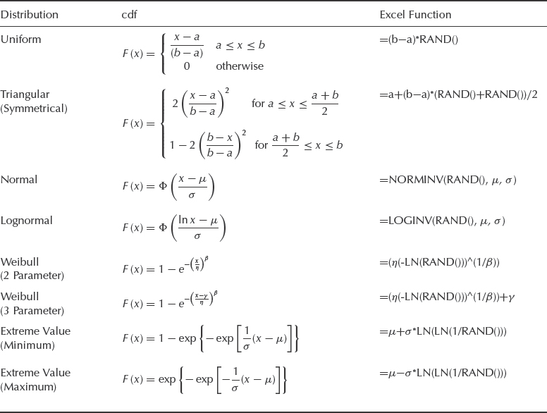
As mentioned before, a basic spreadsheet program can be used to run a Monte Carlo simulation. In this case the generation of random variables is implemented by propagating a basic formula as many times as the number of simulation runs required by the model. For that purpose we need a capability to generate random numbers following the distributions of interest associated with the input variables. Inverse transform sampling is efficient if the cdf can be analytically or computationally inverted, which can be easily done using Excel statistical functions. Even when a distribution does not have a closed-form mathematical expression for cdf, such as the normal or lognormal distributions, it can still be resolved using the Excel inverse statistical function as shown in Table 4.1.

Table 4.1 Statistical distributions sampling using Microsoft Excel¯.

4.4.2 Number of Simulation Runs and the Accuracy of Results

There is no simple way to estimate the number of Monte Carlo simulation runs needed to achieve the required accuracy. The number of runs (also referred as trials, simulations, iterations, or sample size) depends on the complexity of the deterministic model, variance of the input and the sought accuracy of the output. High variance of the input and high complexity of the model increases the variance of the output and thus necessitates more simulation runs to achieve ‘stability’ of the output.

Monte Carlo simulation is a statistical measure; therefore based on the central limit theorem and the confidence bounds estimate for the normal distribution (see Chapters 2 and 3) the standard error of the distribution mean can be expressed as:

where: Er(μ) = standard error of the mean.

Eq. (4.3) can estimate the required number of runs to reach a certain level of confidence in statistics of the simulated output. This equation clearly shows that in order to reduce the error by one order of magnitude the number of runs should be two orders. However Eq. (4.3) has limited applications because the value of σ is not known and can only be assumed a priori or estimated after the first simulation.

Example 4.1

An electric circuit current was modelled with 1000 Monte Carlo simulation runs. The mean value of the outputs is 20 A with the standard deviation of 10 A. Estimate the number of runs required to achieve 1% accuracy with 95% confidence.

For this analysis we need to convert Eq. (4.3) into the percentage format by dividing both sides by μ. This turns σ into the relative standard deviation of 10/20 = 0.5 (50% ) and the desired error of mean Er(μ)/μ into the percentage value of 0.01 (1.0%). For α = 1 − C = 0.05, Z_0.025 = 1.645 (= NORMSINV(0.95) in Excel). Therefore, based on Eq. (4.3) the number of required runs can be calculated as:

As mentioned before, Eq. (4.3) should only be used as an approximation, therefore the number above can only be considered as a rough estimate of the required number of runs.

In order to make the simulation faster and more efficient, MC practitioners often utilize stratified sampling (as opposed to pure random sampling). One popular approach to stratified sampling is called Latin Hypercube Sampling (LHS). In Latin Hypercube Sampling, the range of each input variable is divided into intervals (bins) of equal probability. Then the sampling is performed according to the algorithm where each bin is sampled once before repeating. This algorithm also defines the order in which the samples from the bins are combined between the different input variables. This strategy helps to produce more evenly distributed (in probability) random values and reduce the occurrence of less likely combinations, such as those where all the input variables come from the tails of their respective distributions. Overall LHS generates a set of samples that more precisely reflect the shape of a sampled distribution and the mean of a set of simulation results more quickly approaches the ‘true’ value. Many commercially available Monte Carlo software packages have an option to run Latin Hypercube sampling in addition to the random sampling. Furthermore some of the commercial packages, like @Risk¯ can automatically determine the sufficient number of runs by tracking the convergence of the output during the simulation, see, for example Palisade (2005). For more on LHS and other methods of stratified sampling see Rubinstein and Kroese (2008) and Roberts and Casella (2004).

4.5 Basic Steps for Performing a Monte Carlo Simulation

A Monte Carlo simulation study may be divided into different steps. Those steps could vary based on the scope of the problem, but some basic steps that should be included in any analysis are outlined below:

Step 1: Define the problem and the overall objectives of the study. Evaluate the available data and outcome expectations.

Step 2: Define the system and create a parametric model, γ = f (x₁, x₂, . . ., x_q).

Step 3: Design the simulation. Quantities of interest need to be collected, such as the probability distributions for each of the inputs. Define how many simulation runs should be used. The number of runs, m is affected by the complexity of the model and the sought accuracy of results (Section 4.4.2).

Step 4: Generate a set of random inputs, x_i1, x_i2, . . ., x_iq.

Step 5: Run the deterministic system model with the set of random inputs. Evaluate the model and store the results as y_i.

Step 6: Repeat steps 4 and 5 for i = 1 to m.

Step 7: Analyse the results statistics, confidence intervals, histograms, best fit distribution, or any other statistical measure.

These steps are summarized and depicted in the diagram Figure 4.3.

Example 4.2 Calculating the Probability of Exceeding Yield Strength

In order to illustrate the Monte Carlo method, let us consider a simple stress analysis problem, where a random force F is applied to a rectangular area with dimensions A × B. Based on the previously recorded data and the goodness of fit criteria, force F can be statistically described by the 2-parameter Weibull with β = 2.5 and η = 11 300 N (mean value 10 026 N). Dimension A has the mean value of 2.0 cm with the tolerance of ±1.0 mm and B has the mean of 3.0 cm with the tolerance of ±1.5 mm. The structure is expected to function properly while within the elastic strain range, therefore the probability of exceeding the yield strength of 30 MPa (30 × 10⁶ N/m²) needs to be estimated.

Uniaxial stress can be calculated as the force divided by the area it is acting on:

Despite the apparent simplicity of Eq. (4.4) it would be difficult to calculate analytically even the simplest statistics of the result, such as mean or standard deviation, let alone obtaining the statistical distribution of the resulting stress value. Monte Carlo simulation is perhaps the most efficient way to solve this problem. Following the process described in Section 4.5, the first two steps have defined the problem and created the parametric model (see the previous paragraphs and Eq. (4.4)). Step 3 involves designs of the simulation. While the distribution for the force F is already known, A and B still need to be modelled as random variables due to the dimensional tolerances. There is a number of ways to model a tolerance, and one of them is to use a triangular distribution with the minimum and maximum values corresponding to the minus and plus tolerances. Therefore, A can be defined by the three point estimator: [0.019 (min), 0.02 (most likely), 0.021 (max)] metres and B as [0.0285, 0.03, 0.0315] metres. Considering that there are only three variables in this model, we will start with the relatively low number of iterations m = 1000.

Figure 4.3 Monte Carlo simulation process.

Steps 4 and 5 involve using the Excel spreadsheet as a simulation tool, as shown in Figure 4.4. Let us start with entering the variables' names: A (m), B (m), F (m), and S (Pa) respectively in row 1. In row 2 we write the equations for their respective random variables.

Then each of the cells A2 through D2 is copied down through row 1001. Depending on the Excel calculation settings, it may be required to hit the ‘recalculate’ key (often F9 in Windows applications) to generate the random variables. At this point, the process of simulation (step 6) is complete and the output values are generated in column D. In order to estimate the probability of S exceeding 30 MPa we need to calculate the ratio of the cells with the stress values greater than 30 MPa (S > 30 000 000) to the total number of cells generated during the simulation. It can be easily done with the Excel formula:

Figure 4.4 Monte Carlo Simulation using Microsoft Excel¯.

One of the ways to assess the sufficiency of the number of runs (number or generated rows in this example) is to repeatedly hit ‘Recalculate’ (typically F9) and observe the value of the ratio (4.5). In this case, this procedure produced a random sequence of numbers (4.6; 3.7; 4.1; 3.95; 4.25; 4.05; 4.3; 4.55; 4.1; 3.5; 4.1; 4.05) with the average of 4.104%. To complete the analysis the generated output values in column D can be presented as a histogram or plotted as a cdf of the resulting distribution. The standard deviation of the data in column D can also be used to calculate the number of required simulation runs (Excel rows) per Eq. (4.3). For this purpose we would need to specify the required accuracy and the confidence level, similar to that in Example 4.1.

In order to run a more sophisticated analysis we can employ commercially available software, such as @Risk¯. @Risk works off a standard Excel spreadsheet. All the random numbers are compactly generated in their respective single cells (both inputs and outputs). It provides the option of graphical representation of the input variables and the histogram generation of the output. Table 4.2 shows the input variables F, A, B graphically generated with @Risk software.

Completing this simulation with 10 000 runs took approximately 30 seconds. The output values were automatically presented as a histogram with the best fitting distribution shown in Figure 4.5. This distribution according to both Chi-square and Kolmogorov-Smirnov criteria was 3 parameter Weibull with β = 2.48, η = 18.8 × 10⁶ Pa, γ = 38 593 Pa). The right tail of this distribution in Figure 4.5 also shows that in 4.2% of the cases the stress S exceeded 30 MPa.

In addition to the basic simulation, the sensitivity analysis was completed with the results shown in Figure 4.6. This analysis helps to determine how sensitive the output is to variations in each input.

Figure 4.6 shows that based on the correlation coefficients the output S is approximately eight times more sensitive to variations in force value (F) than to variation in the cross sectional dimensions. That happened due in part to a much larger variation of the random variable F than that of either A or B. Both A and B have their values restricted by the highest and lowest values, where force F can theoretically be very high due to the tail of the Weibull distribution.

4.6 Monte Carlo Method Summary

Over the years the Monte Carlo method has proven itself as a very useful tool in a variety of applications involving uncertainty. However it is important for a practitioner to understand the advantages and disadvantages of using Monte Carlo simulation in problem solving.

The main advantage of the method is based on its low level of complexity. Compared to the other numerical methods that can solve the same problem, MC is conceptually very simple and is relatively easy to implement on a computer. It does not require specific knowledge of the form of the solution or its analytic properties. It does not constrain what form the distributions take, and the distributions need not necessarily even have a mathematical representation. The Monte Carlo method is useful for modelling phenomena with significant uncertainty in inputs and it always works regardless of the complexity of the model.

Another important advantage is the ease of comprehension by decision-makers. ‘What-if’ scenarios and the sensitivity of the outputs to input assumptions can be quickly analysed.

Table 4.2 Input variables generated by @Risk¯ for Example 4.2 (Reproduced by permission of Palisade Corporation).

Figure 4.5 Simulation results including the histogram and the best fit distribution for Example 4.2 using @Risk v.5.7 (Reproduced by permission of Palisade Corporation).

Figure 4.6 Monte Carlo Simulation sensitivity analysis by @Risk¯ (Reproduced by permission of Palisade Corporation).

The disadvantages of using Monte Carlo include computational intensity, especially with complex models requiring large numbers of simulation runs, although with growing computing power, this becomes less of a problem. The arguments against Monte Carlo also include claims that it is a ‘brute force’ solution heavily relying on computer power. Furthermore, it is difficult to estimate an error, since there are no hard bounds on the error of the computed result. The probabilistic error bound, which is essentially based on the variance, may not be a good measure of the error, especially for skewed distributions. Another potential drawback is that Monte Carlo implicitly assumes that all the parameters are independent, which may not be the case, especially with complex models. Correlated inputs should be identified in advance and simulated as such; otherwise the simulation may produce biased results.

Faulin et al. (2010) describe simulation applications to complex systems reliability and availability.

Questions

The following problems can be solved using Excel spreadsheet. A trial version of @Risk software can be downloaded from http://www.palisade.com/ or this textbook's version from http://www.palisade.com/bookdownloads/oconnorkleyner for more sophisticated analysis.

1. Program 2-paramter Weibull distribution with β = 3.0 and η = 1000 into Excel spreadsheet and generate 100 rows by copying down the equation from Table 4.1. In the next column generate 1000 rows and in the next column 10 000 rows. Calculate the mean and standard deviation for each column. By hitting ‘Recalculate’ (typically F9) observe the mean and standard deviation values. What can you say about the variation for each group?
2. When simulating the function Z = X^Y where X and Y are random functions. If X and Y are comparable statistical distribution (e.g. both normal with μ = 10.0, σ = 2.0), will the function Z be more sensitive to X or Y? Justify your answer.
3. Derive an Excel formula to simulate a non-symmetrical version of triangular distribution shown in Table 4.1.
4. Estimate top one-sided 80% confidence on warranty claims cost of a washing machine. Warranty cost can be calculated as (Sales Volume)×C_W×(1-NFF)×[1-R(3yrs)], where C_W is the cost per warranty claim, R(3yrs) is reliability at 3 years and NFF is the percent of ‘no fault found’ claims. Sales volume is uniformly distributed between 800 000 and 1 million units. Cost of warranty is lognormally distributed with the parameters μ = 5.8 and σ = 0.5. The washing machine has a constant failure rate, which can be between 0.001 and 0.002 failures per year (uniformly distributed). NFF can be modelled by a symmetrical triangular distribution with the minimum and maximum values of 20 and 50%.

   If you are using @Risk or other specialized Monte Carlo simulation software, run a sensitivity analysis and determine which variable has the most impact on the total warranty cost.

5. Suppose that you have run a Monte Carlo analysis (m samples) and wish to cut the standard deviation in half. How many samples do you need to run?
6. Test the hypothesis that whenever several random variables are added together, the resulting sum tends to normal regardless of the distribution of the variables being added. Sample the sum of 10 random variables from different statistical distribution and test the normality of this sum by constructing the histogram or using other statistical tools.
7. An electric circuit current was modelled with 1000 experiments. The mean value of the outputs is 25 amps with the standard deviation of 8 amps. Estimate the number of runs required to achieve 1% accuracy with 95% confidence.

Bibliography

Faulin, J., Juan, A., Martorell, S. and Ramírez-M´arquez, J.-E. (eds) (2010) Simulation Methods for Reliability and Availability of Complex Systems, Springer-Verlag.

Hazelrigg, G. (1996) Systems Engineering: An Approach to Information-Based Design, Prentice Hall.

Palisade (2005) Guide to Using @Risk. Advanced Risk Analysis for Spreadsheets, Palisade Corporation, Newfield, New York. Available at: http://www.palisade.com (Accessed February 2011).

Roberts, C. and Casella, G. (2004) Monte Carlo Statistical Methods, 2nd edn, Springer.

Rubinstein R. and Kroese D. (2008) Simulation and the Monte Carlo Method, 2nd edn (Wiley Series in Probability and Statistics), Wiley.

Sandborn, P. (2011) Electronic Systems Cost Modeling – Economics of Manufacturing and Life Cycle. Chapter 10 (Uncertainty Modeling). World Scientific Publishing, Co.

Wikipedia (2010) Inverse Transform Sampling: Available at: http://en.wikipedia.org/wiki/Inverse_transform_sampling.