13

Analysing Reliability Data

13.1 Introduction

This chapter describes a number of techniques, further to the probability plotting methods described in Chapter 3, which can be used to analyse reliability data derived from development tests and service use, with the objectives of monitoring trends, identifying causes of unreliability, and measuring or demonstrating reliability.

Since most of the methods are based on statistical analysis, the caution given in Section 2.17 must be heeded, and all results obtained must be judged in relation to appropriate engineering and scientific knowledge.

13.2 Pareto Analysis

As a first step in reliability data analysis we can use the Pareto principle of the ‘significant few and the insignificant many’. It is often found that a large proportion of failures in a product are due to a small number of causes. Therefore, if we analyse the failure data, we can determine how to solve the largest proportion of the overall reliability problem with the most economical use of resources. We can often eliminate a number of failure causes from further analysis by creating a Pareto plot of the failure data. For example, Figure 13.1 shows failure data on a domestic washing machine, taken from warranty records. These data indicate that attention paid to the program switch, the outlet pump, the high level switch and leaks would be likely to show the greatest payoff in warranty cost reduction. However, before committing resources it is important to make sure that the data have been fully analysed, to obtain the maximum amount of information contained therein. The data in Figure 13.1 show the parts replaced or adjusted.

In this case further analysis of records reveals:

1. For the program switch: 77 failures due to timer motor armature open-circuit, 18 due to timer motor end bearing stiff, 10 miscellaneous. Timer motor failures show a decreasing hazard rate during the warranty period.
2. For the outlet pump: 79 failures due to leaking shaft seal allowing water to reach motor coils, 21 others. Shaft seal leaks show an increasing hazard rate.
3. For the high level switch: 58 failures due to failure of spot weld, allowing contact assembly to short to earth (decreasing hazard rate), 10 others.

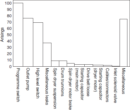
Figure 13.1 Pareto plot of failure data.

These data reveal definite clues for corrective action. The timer motor and high level switch appear to exhibit manufacturing quality problems (decreasing hazard rate). The outlet pump shaft leak is a wear problem (increasing hazard rate). However, the leak is made more important because it damages the pump motor. Two types of corrective action might be considered: reorientation of the pump so that the shaft leak does not affect the motor coils and attention to the seal itself. Since this failure mode has an increasing rate of occurrence relative to equipment age, improving the seal would appreciably reduce the number of repair calls on older machines. Assuming that corrective action is taken on these four failure modes and that the improvements will be 80% effective, future production should show a reduction in warranty period failures of about 40%.

The other failure modes should also be considered, since, whilst the absolute payoff in warranty cost terms might not be so large, corrective action might be relatively simple and therefore worthwhile. For example, some of the starting capacitor failures on older machines were due to the fact that they were mounted on a plate, onto which the pump motor shaft leak and other leaks dripped. This caused corrosion of the capacitor bodies. Therefore, rearrangement of the capacitor mounting and investigation into the causes of leaks would both be worth considering.

This example shows the need for good data as the basis for decision-making on where to apply effort to improve reliability, by solving the important problems first. The data must be analysed to reveal as much as possible about the relative severity of problems and the likely causes. Even quite simple data, such as a brief description of the cause of failure, machine and item part number, and purchase date, are often enough to reveal the main causes of unreliability. In other applications, the failure data can be analysed in relation to contributions to down-time or by repair cost, depending upon the criteria of importance.

13.3 Accelerated Test Data Analysis

Failure and life data from accelerated stress tests can be analysed using the methods described in Chapters 2, 3, 5 and 11. If the mechanism is well understood, for example material fatigue and some electronic degradation processes, then the model for the process can be applied to interpret the results and to derive reliability or life values at different stress levels. Also, the test results can be used to determine or confirm a life model. The most commonly used stress–life relationship models include:

In this model there is an exponential relationship between the life (or other performance measure) and the stress. A is an empirical constant and X can be a constant or function describing this relationship (more later in this chapter). Depending on the failure mechanism, stress can be a maximum application temperature, temperature excursion ΔT during thermal cycling, vibration G_RMS, humidity, voltage and other external or internal parameters. Failure mechanisms of electronic components typically follow this relationship over most of their life for dependence on temperature. Some materials follow this type of relationship as a function of weathering.

In this model there is a simple power relationship between the performance measure and the stress variable. Failure mechanisms of electronic components typically follow this relationship over most of their life for dependence on voltage. Electric motors follow a similar form for dependence on stresses other than temperature. Mechanical creep of some materials may follow a form such as this.

There are other models including the mix of exponential and power model or other physical laws. Some of these models are covered in detail in this chapter.

13.4 Acceleration Factor

Most life-stress models (see (13.1) and (13.2)) contain an empirical constant A, which is usually unknown a priori and can only be obtained by testing for a specific failure mechanism under specific test conditions. Also the measure of life will affect the value of A, for example product's life can be measured as MTBF, MTTF, B₁₀-life, Weibull characteristic life η or even as time to the first failure. Therefore, it is more common to analyse test data based on acceleration factor, AF.

Where L_Field is the product life at the field stress level and L_Test is the life at the test (accelerated) stress level. Other literature may use different nomenclature, such as L_U (use) for field life and L_S (stress) or L_A (accelerated) for test life. In (13.3) the acceleration factor is independent of the empirical constant A and of the measure of product life. The relationship (13.3) assumes the same failure mechanism caused by the same type of environment only at a different stress level.

The effect of accelerated test conditions on product life has been illustrated in Chapter 12, bathtub curve, Figure 12.7, therefore acceleration factor is used to calculate the required test time based on the expected product field life. Acceleration factor effect on the key reliability functions is shown in Table 13.1. The ability to calculate the acceleration factor is critical to the development of an efficient test plan adequately reflecting the field level stress conditions.

Table 13.1 Acceleration factor relationship with reliability functions.

Example 13.1

Mean time to failure (MTTF) for a microprocessor at the field level temperature of 60 °C is 20 years assuming 2 hours of operation per day. Continuous test at 120 °C produced failure modes consistent with field failures and the MTTF = 1000 hours. Calculate the acceleration factor.

In order to calculate the field life we need to convert 20-year life into the number of operating hours: L_Field = 20 years × 365 days/year × 2 hours/day = 14 600 hours

13.5 Acceleration Models

This section discusses the acceleration models attributed to various stresses such as temperature, humidity, vibration, voltage and current. All those models contain empirical constants most of which are generic values for the specific models and specific failure mechanisms. These generic constants are obtained from past experience or past testing. Even though these constants have been widely used in the industry for many years, it is always best to obtain these empirical values by conducting test to failure experiments at different stress levels and fitting the obtained life data into a model. The development of acceleration models based on accelerated test data is discussed in Section 13.7.

13.5.1 Temperature and Humidity Acceleration Models

Following are the most commonly used acceleration models involving stresses caused by temperature and humidity.

13.5.1.1 Arrhenius Model

Based on the Arrhenius Eq. (8.5), life is non-linear in the single stress variable, temperature (T). It describes many physical and chemical temperature-dependent processes, including diffusion and corrosion. The Arrhenius model has various applications, but it is most commonly used to estimate the acceleration factor for electronic component operation at a constant temperature:

E_A = activation energy for the process.

k = 8.62 × 10⁻⁵ eV/K (Boltzmann constant).

T_Field and T_Test = absolute Kelvin temperatures at field and test level respectively.

The original definition of Arrhenius' activation energy E_A came from chemistry and physics. It corresponds to the minimum energy required for the electron to move to a different energy level and begin a chemical reaction. It is important to note that even though E_A has a specific meaning as an atomic or material property, in the Arrhenius equation it simply becomes an empirical constant appropriate for use with a particular failure mechanism. This means that at a component level activation energy is not a simple material property but a fairly complex function of geometry, material properties, technology, interconnections and other factors. Therefore it is sometimes referred as E_AA – ‘apparent activation energy’ (JEDEC, 2009).

There are no predetermined generic values of E_A for the specific failure mechanisms due to variation in parts characteristics, therefore different reference sources list different values for the activation energies. However some recommended values suggested in the literature on the subject (see, e.g. Ohring, 1998) are listed in Table 13.2.

Please note, that the only reliable way to obtain the value of E_A is to conduct a series of accelerated tests and record failure times as a function of temperature (see Example 13.4). It is also important to note that the Arrhenius acceleration factor is very sensitive to the value of E_A due to its exponential nature, therefore the accuracy of estimating E_A is important.

Table 13.2 Commonly used activation energy values for different failure mechanisms.

Failure Mechanism	Activation Energy, EA (eV)
Gate oxide defect	0.3–0.5
Bulk silicon defects	0.3–0.5
Silicon junction defect	0.6–0.8
Metallization defect	0.5
Au-Al intermetallic growth	1.05
Electromigration	0.6–0.9
Metal corrosion	0.45–0.7
Assembly defects	0.5–0.7
Bond related	1.0
Wafer fabrication (chemical contamination)	0.8–1.1
Wafer fabrication (silicon/crystal defects)	0.5–0.6
Dielectric breakdown, field > 0.04 micron thick	0.3
Dielectric breakdown, field <= 0.04 micron thick	0.7
Adhesive tack: bonding-debonding	0.65–1.0

13.5.1.2 Eyring Model

The Eyring model is usually applied to combine the effect of more than one independent stress variable assuming no interactions between the stresses. Many other models are simplified versions of the Eyring model. A generic form of the Eyring equation is

Y₁(Stress1), Y₂(Stress2) are the factors for other applied stresses, such as temperature, humidity, voltage, current, vibration, and so on.

A form of the Eyring model for the influence of voltage, V in addition to temperature is:

To use this formula, four constants, A, B, C, D must be known or estimated (see NIST, 2006).

13.5.1.3 Peck Temperature-Humidity Model

As a special case of the Eyring model, Peck's equation (Peck, 1986) is probably the most commonly used acceleration model addressing the combined effect of temperature and humidity. According to Peck, the acceleration factor correlating product life in the field with test duration can be expressed as:

where: m = humidity power constant, typically ranging between 2.0 and 4.0

Despite the limited applications and varying accuracy, Peck's model has been often utilized to calculate field-to-test ratios for a wide variety of products and failure modes. It is important to note that this model can only be applied to wear-out failure mechanisms, including electromigration, corrosion, dielectric breakdown and dendritic growth (Kleyner, 2010a). It has also been applied to tin whisker growth in lead-free electronics, although with varying degrees of success.

13.5.1.4 Lawson Temperature-Humidity Model

A lesser known temperature-humidity model, which is based on the water absorption research presented in Lawson (1984) is often applied its modified version:

b is an empirical humidity constant based on water absorption. In many electronics applications involving silicon chips b = 5.57×10⁻⁴ although it is best when b is determined based on test results.

13.5.1.5 Tin-Lead Solder

Solder joint fatigue has always been a source of concern in the electronics industry (Chapter 9). The well-known Coffin-Manson relationship provides a relationship between life in thermal cycles, N, and plastic strain range Δγ_p.

m is an empirical fatigue constant, observed to be about 2.0–3.0 for eutectic tin-lead solder.

During thermal cycling the strain range caused by the mismatch of the coefficients of thermal expansion between solder and other materials is proportional to the cycling temperature excursion ΔT = T_Max − T_Min. Based on (13.9) the acceleration factor can be approximated by:

In the case of low cycle fatigue, the acceleration factor is typically applied to the number of thermal cycles rather than the temperature exposure time. There are extensions of the Coffin-Manson model which account for the effect of temperature transition during thermal cycling (see Norris and Landzberg, 1969). However, there is no conclusive evidence that faster temperature transition has a significant effect on fatigue life of tin-lead solder joints.

13.5.1.6 Lead-Free Solder

As mentioned in Chapter 9, lead-free solder mechanical behaviour is different from that of tin-lead including its low cycle fatigue properties. Simplified lead free model is based on the tin-lead coffin Manson equation (13.10) with the fatigue constant m = 2.6 – 2.7. However, the research showed that lead-free solder acceleration factors are also influenced by the variables other than ΔT, such as the maximum and minimum cycling temperatures, dwell times (both at maximum and minimum temperatures) and to some degree the temperature transition rate.

As mentioned in Chapter 9, lead-free solder has not been studied for nearly as long as tin-lead, therefore it will take time before technical knowledge about lead-free solder reaches maturity. Several empirical lead-free acceleration models have been developed in the last years, especially for SAC305 solder. Some of these models are covered in Pan et al. (2005), Clech et al. (2005), Salmela (2007) and several more are still in the process of development.

13.5.2 Voltage and Current Acceleration Models

A simple inverse power law model often used for capacitors has only voltage V dependency and takes the form:

An alternative exponential voltage model takes the form of:

Where B is voltage acceleration parameter (typically determined from an experiment). The exponential voltage model (13.12) combined with Arrhenius can be applied to time dependent dielectric breakdown (TDDB) (JEDEC, 2009) in the form of:

Another form of the Eyring equation can be used to model electromigration (Section 9.3.1.5). The ionic movement is accelerated by high temperatures and increased current density, J.

The commonly used values for Al or Al-Cu alloys E_A = 0.7 – 0.9 eV and n = 2.

More acceleration models for electronic devices can be found in SEMATECH, 2000.

13.5.3 Vibration Acceleration Models

Most vibration models are based on the S-N curve introduced in Chapter 8. The relationship between peak stress σ and the number of cycles to failure, N can be expressed as Nσ^b = Constant (high cycle fatigue). Assuming the linear relationship between the stress and acceleration G during vibration, the model takes the form:

Fatigue exponent b is the slope of the S-N line in the log-log scale (Chapter 8, Figure 8.5) and has different values for different materials (see Steinberg, 2000 for fatigue curves). b = 4.0 – 6.0 is very common for electronics related failure (electrical contacts, component leads, mounting brackets, etc.) It is typical for sinusoidal vibration to measure life in vibration time or a number of cycles. For random vibration it is the test time or the number of stress reversals (see Steinberg, 2000).

Example 13.2

An electrical insulator is rated for normal use at 12 kV. Prior tests of a sample have suggested this insulator will operate over 30 kV and a stress-life exponent of the power model was found to be N = 5.5. How long must one run an accelerated life test at 30 kV to demonstrate an equivalent B₁₀ life (based upon voltage only) if the B₁₀ life at 12 kV is desired to be at least 25 years?

Let life, L = A(V)^−N represent the typical stress life relationship (inverse power law).

Applying (13.11) to calculate the acceleration factor due to voltage only:

Therefore:

Extrapolation of accelerated test results to expected in-service conditions can be misleading if the test stresses are much higher, since different failure mechanisms might be stimulated. That increases the probability of irrelevant or ‘foolish’ failures. This is particularly the case if very high stresses, particularly combined stresses, are applied, as in HALT (Chapter 12). It is important that the primary objective of the test is understood: whether it is to determine or confirm a life characteristic, or to help to create designs that are inherently failure free.

Life characteristics such as those listed above can only be analysed when the data represent a single (or dominant) failure mode. This significantly complicates the analysis of failures of assemblies or systems, when several different failure modes might be present. In those cases, different failure modes need to be addressed by a series of environmental tests targeting individual failure mechanisms as presented in Section 12.5. Life-stress models then should be applied to every stress environment in that test programme in order to calculate the appropriate test durations (see the next section).

Life data analysis methods (Chapter 3) at different stress levels can also be used for analysing such data when sufficient data are available (see Section 13.7).

13.6 Field-Test Relationship

Determining what a particular test represents in terms of the field life of a product and vice versa can often be a complicated task. It combines the use of the appropriate acceleration models with knowledge of the stress and usage conditions in the field. As mentioned before, an acceleration model should be applied only to one failure mechanism at a time, however in reality there are almost always more than one potential failure mechanism present. Therefore it is practicable to address the most dominant failure mechanism associated with a particular environment for a particular test in the testing programme (see Chapter 12, Figure 12.9). Additionally, the acceleration factor calculations should account for the failure mechanism which will make the product fail fastest. For example, amongst possible failure mechanisms caused by a constant temperature, the one with the lowest E_A (see Table 13.2) should be selected for the test time calculations because it would yield the most conservative (lowest) acceleration factor.

Design of the test plan simulating the expected product field life should include the following steps:

• Evaluate the stress level and the usage profile for the field environment.
• Select the appropriate acceleration model(s) for the test based on the expected failure mechanism.
• Define the appropriate stress level and test duration based on the test equipment capability and the maximum allowable stress level to avoid ‘foolish’ failures.
• Calculate the acceleration factor and duration of the test based on field stress level and the environmental exposure time during the life time operation.
• Repeat this procedure for each applicable test/environment.

Example 13.3

Develop the thermal cycling test for an automotive controller designed to operate for 10 years and mounted under the hood of a passenger car. First, we need to determine the typical field environment and the usage for this electronic controller. It has been established that two ‘cold’ temperature cycles per day are typical for a 90–98 percentile user of a passenger car. One ‘cold’ cycle represents a vehicle start after being parked at below-freezing temperature and followed by at least 30 minutes of continuous driving. Therefore the 10 year field exposure can be calculated as:

Solder fatigue is often considered to be the dominant failure mechanism for automotive electronics during thermal cycling. Automotive thermal cycling is typically caused by the engine heat combined with the internal heat dissipation of the electronic unit. Therefore the Coffin-Manson model (13.8) is selected to calculate the acceleration factor with m = 2.5 for tin-lead solder. To calculate the acceleration factor we need to know the temperature excursion ΔT for both test and field conditions. Based on the environmental chamber capability and previous experience [−40; +125] °C cycle has been selected. Field study showed that the internal temperature of the under-the-hood-mounted electronics operated in severe climates grows by up to ΔT_Field = 70 °C during driving. Substituting these numbers into (13.8) produces:

Therefore, 856 thermal cycles of [-40; +125] °C will represent one product life of 10 years for an automotive controller mounted under the hood of a vehicle.

13.7 Statistical Analysis of Accelerated Test Data

As mentioned before, the acceleration models discussed in this chapter have limited accuracy because their empirical equations are based on generic data. Therefore, it is always better to develop an acceleration model based on experimental data rather than generic equations. There is commercially available software designed to analyse accelerated life data. When sufficient data is available software packages such as ReliaSoft ALTA¯ or WinSMITH¯ can fit a statistical distribution to a life data set at each stress level and model the resulting life-stress relationship.

An effective quantitative accelerated life test produces life data obtained at two or more stress levels that cause the product to fail. Analysing this data, which contains failed and not failed (suspended) parts we can estimate the parameters for the lifetime distribution that best fits the data at each stress level (e.g. Weibull, exponential, lognormal, etc.). The life-stress relationship then can be used to estimate the pdf at the field use (not accelerated) stress level based on the characteristics of the distributions at each accelerated stress level. A simplified version of this approach is shown in Table 13.1 for the pdf.

The data analyst must first choose a life-stress relationship which is appropriate for the test failure modes and find the best fit to the data being analysed. The appropriate life characteristic can be chosen based on the statistical distribution or other criteria. For example, for the Weibull distribution, the scale parameter η is considered to be stress- dependent. Therefore, the life-stress model for data that fits the Weibull distribution is assigned to η. For the exponential distribution it is MTTF, for the normal it is the mean life, and so on.

As mentioned before, life-stress relationships are specific to the types of failures; therefore it is important that the failure mechanisms remain the same at different stress levels. The best way to verify, this is to perform failure analysis, which often involves cross-sectioning of the failed part. The analytical alternative (though less preferred than failure analysis) is to compare the Weibull slopes β at different stress levels. If the β slope remains constant over the different stress levels of acceleration, it is a good indicator that the product is experiencing the same or similar failure modes.

Table 13.3 Accelerated test results (Example 13.4).

Example 13.4

In order to expedite product development, 24 electronic parts, which are designed to operate at field temperatures up to 40 °C have been subjected to accelerated testing. The first group of eight samples have been tested at 60 °C (333K), second group at 80 °C (353K) and third at 100 °C (373K). The test was terminated after 250 hours. The time-to-failure and time-to-suspension data obtained during this test are presented in Table 13.3.

Assuming the Arrhenius temperature model, calculate the activation energy E_A and determine the life-stress relationship for this device. Based on the accelerated test data, what is the reliability of this part after 100 hours of operation at the field temperature of 40 °C (313K)?

First step is to run life data analysis at each stress level and verify that the parts have the same failure modes at all three temperatures. Figure 13.2 shows the Weibull plots for each group of parts. It shows three approximately equal Weibull slopes, which confirms the consistency of the failure mechanisms at all three stress levels.

The next step is to model the life-stress relationship. In this case we will make use of the ReliaSoft ALTA¯ software which estimates the parameters of the Weibull distributions at each stress level and intrapolates them to the field use level Figure 13.3.

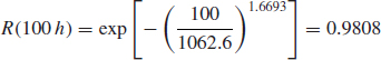
Figure 13.3 shows the distributions at each stress level and model the median life as the function of temperature. Based on the ALTA¯ analysis (Figure 13.3), the activation energy E_A = 0.476, β = 1.6693 and the life stress relationship is:

Characteristic life at the use temperature is η(313K) = 1062.6 h, therefore based on Weibull equation:

Please note that life-stress relationship in this example could be derived using other analytical tools. Characteristic life values calculated using life data analysis (Figure 13.2) at different stress levels η(333K) = 310.0, η(353K) = 169.7, η(373K) = 57.6 can be fitted with the Arrhenius model using Excel spreadsheet. However, specially designed software, such as ALTA¯ can complete this task more efficiently and with higher accuracy.

Figure 13.2 Weibull plot at three stress levels (Weibull++¯) (reproduced by permission of ReliaSoft.

Figure 13.3 Life vs. stress plot generated with ALTA¯ software (reproduced by permission of ReliaSoft).

13.8 Reliability Analysis of Repairable Systems

13.8.1 Failure Rate of a Repairable System

Chapter 3 described methods for analysing data related to the time to first failure. The distribution function of times to first failure are obviously important when we need to understand failure processes of parts which are replaced on failure, or when we are concerned with survival probability, for example, for missiles, spacecraft or underwater telephone repeaters.

However, for repairable systems (Chapters 2 and 6), which represent the majority of everyday reliability experience, the distribution of times to first failures are much less important than is the failure rate or rate of occurrence of failures (ROCOF) of the system.

Any repairable system may be considered as an assembly of parts, the parts being replaced when they fail. The system can be thought of as comprising ‘sockets’ into which non-repairable parts are fitted. We are concerned with the pattern of successive failures of the ‘sockets’. Some parts are repaired (e.g. adjusted, lubricated, tightened, etc.) to correct system failures, but we will consider first the case where the system consists only of parts that are replaced on failure (e.g. most electronic systems). Therefore, as each part fails a new part takes its place in the ‘socket’. If we ignore replacement (repair) times, which are usually small in comparison with standby or operating times, and if we assume that the time to failure of any part is independent of any repair actions, then we can use the methods of event series analysis in Chapter 2 to analyse the system reliability.

Consider the data of Example 2.19, Section 2.15.1. The interarrival and (chronologically ordered) arrival values between successive component failures were as shown in columns 1 and 2:

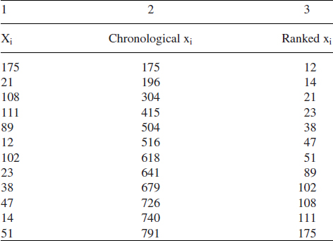
Example 2.19 showed that the failure rate was increasing, the interarrival values tending to become shorter. In other words, the interarrival values are not IID. If, however, we had not performed the centroid test and assumed that the data were IID, we might order the data in rank order (column 3) and plot on probability paper. These are shown plotted on Weibull paper in Figure 13.4 (Line A). The plot shows an apparently exponential component life distribution. This is obviously a misleading result, since there is clearly an increasing failure rate trend for the ‘socket’ when the data are studied chronologically.

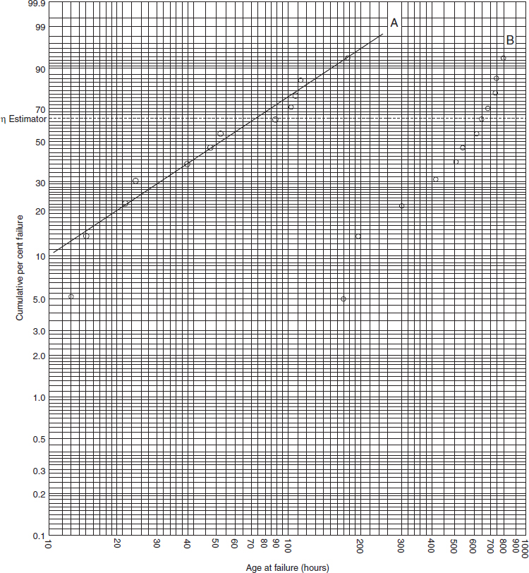
Figure 13.4 Plotted data of Example 2.19.

This example shows how important it is for failure data to be analysed correctly, depending on whether we need to understand the reliability of a non-repairable part or of a repairable system consisting of ‘sockets’ into which parts are fitted. The presence of a trend when the data are ordered chronologically shows that times to failure are not IID, and ordering by magnitude, which implies IID, will therefore give misleading results. Whenever failure data are reordered all trend information is ignored. The appropriate method to apply is trend (time series) analysis.

We can derive the system reliability over a period by plotting the cumulative times to failure in chronological order (column 2) rather than in rank order. This is shown in Figure 13.4 (Line B). It shows the progressively increasing failure rate (though the ‘socket’ times to failure are not Weibull-distributed).

13.8.2 Multisocket Systems

Now we will consider a more typical system, comprised of several parts which exhibit independent failure patterns. Each part fills a ‘socket’. The failure pattern of such a system, comprising six ‘sockets’, is shown in Figure 13.5.

Socket 1 generates a high, constant rate of system failures. Socket 2 generates an increasing rate of system failures as the system ages, and so on. The combined failure rate can be seen on the bottom line. The estimate of U (see the centroid test Chapter 2 Eq. (2.46)) for each part and for the system is shown. When U is negative (i.e. negative process trend), it denotes a ‘happy’ socket, with an increasing inter-arrival time between failures (decreasing failure rate, DFR). A positive value of U indicates a ‘sad’ socket (increasing failure rate, IFR).

If there are no perturbations (which will be discussed below) the failure rate will tend to a constant value after most parts have been replaced at least once, regardless of the failure trends of the sockets (see Example 2.19) This is one of the main reasons why the constant failure rate, CFR assumption has become so widely used for systems, and why part hazard rate has been confused with failure rate. However, the time by which most parts have been replaced in a system is usually very long, well beyond the expected life of most systems.

Figure 13.5 The failure pattern of a multisocket system.

If part times to failure (in a series system, see Chapter 6) are independently and identically exponentially distributed (IID exponential) the system will have a CFR which will be the sum of the reciprocals of the part mean times to failure, that is

The assumption of IID exponential for part times to failure within their sockets in a repairable system can be very misleading. The reasons for this are (adapted from Ascher and Feingold, 1984 with permission):

1. The most important failure modes of systems are usually caused by parts which have failure probabilities which increase with time (wearout failures).
2. Failure and repair of one part may cause damage to other parts. Therefore times between successive failures are not necessarily independent.
3. Repairs often do not ‘renew’ the system. Repairs are often imperfect or they introduce other defects leading to failures of other parts.
4. Repairs might be made by adjustment, lubrication, and so on, of parts which are wearing out, thus providing a new lease of life, but not ‘renewal’, that is, the system is not made as good as new.
5. Replacement parts, if they have a decreasing hazard rate, can make subsequent failure initially more likely to occur.
6. Repair personnel learn by experience, so diagnostic ability (i.e. the probability that the repair action is correct) improves with time. Generally, changes of personnel can lead to reduced diagnostic ability and therefore more reported failures.
7. Not all part failures will cause system failures.
8. Factors such as on–off cycling, different modes of use, different system operating environments or different maintenance practices are often more important than operating times in generating failure-inducing stress.
9. Reported failures are nearly always subject to human bias and emotion. What an operator or maintainer will tolerate in one situation might be reported as a failure in another, and perception of failure is conditioned by past experience, whether repair is covered by warranty, and so on. Wholly objective failure data recording is very rare.
10. Failure probability is affected by scheduled maintenance or overhaul. Systems which are overhauled often display higher failure rates shortly after overhaul, due to disturbance of parts which would otherwise not have failed. If there is a post-overhaul test period before the system is returned to service, many of these failures might be repaired then. The failure data might or might not include these failures.
11. Replacement parts are not necessarily drawn from the same population as the original parts – they may be better or worse.
12. System failures might be caused by parts which individually operate within specification (i.e. do not fail) but whose combined tolerances cause the system to fail.
13. Many reported failures are not caused by part failures at all, but by events such as intermittent connections, improper use, maintainers using opportunities to replace ‘suspect’ parts, and so on.
14. Within a system not all parts operate to the overall system cycle.

Any practical person could add to this list from his or her own experience. The factors listed above often predominate in systems to be modelled and in collected reliability data. Large data-collection systems, in which failure reports might be coded and analysed remotely from the work locations, are usually most at fault in perpetrating the analytical errors described. Such data systems might generate ‘MTBFs’ for systems and for parts by merely counting total reported failures and dividing into total operating time. For example, MTBFs in flying hours are quoted for aircraft electronic equipment, when the equipment only operates for part of the flight, or MTBFs in hours are quoted for valves, ignoring whether they are normally closed, normally open or how often they are opened and closed. These data are often used for reliability predictions for new systems (see Chapter 6), thus adding insult to injury.

A CFR is often a practicable and measurable first-order assumption, particularly when data are not sufficient to allow more detailed analysis.

The effect of successive repairs on the reliability of an ageing system are shown vividly in the next example (from Ascher and Feingold, 1984).

Example 13.5 (Reprinted from Ascher and Feingold (1984) by courtesy of Marcel Dekker, Inc.)

Data on the miles between major failures (interarrival values) of bus engines are shown plotted in Figure 13.6. These show the miles between first, second, . . ., fifth major failure. Note that the interarrival mileages to the first failures (X_i) are nearly normally distributed. Successive interarrival times (second, third, fourth, fifth failures) show a tendency to being exponentially distributed. Nevertheless, the results show clearly that the reliability decreases with successive repairs, since the mean of the interarrival distances is progressively reduced:

Failure No.	miles
1	94 000
2	70 000
3	54 000
4	41 000
5	33 000

The importance of this result lies in the evidence that:

1. Repair does not return the engines to an ‘as new’ condition.
2. Successive X_i s are not IID exponential.
3. The failure rate tends to a constant value only after nearly all engines have been repaired several times. Even after five repairs the steady state has not been reached.
4. Despite the appearance of ‘exponentiality’ after several failures, replacement or more effective overhaul appears to be necessary.

13.9 CUSUM Charts

The ‘cumulative sum’, or CUSUM, chart is an effective graphical technique for monitoring trends in quality control and reliability. The principle is that, instead of monitoring the measured value of interest (parameter value, success ratio), we plot the divergence, plus or minus, from the target value. The method is the same as the scoring principle in golf, in which the above or below par score replaces the stroke count. The method enables us to report progress simply and in a way that is very easily comprehended.

The CUSUM chart also provides a sensitive indication of trends and changes. Instead of indicating measured values against the sample number, the plot shows the CUSUM, and the slope provides a sensitive indicator of the trend, and of points at which the trend changes.

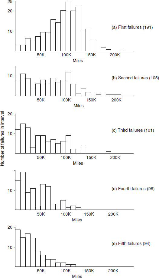
Figure 13.6 Bus engine failure data (a) First failures (191), (b) Second failures (105), (c) Third failures (101), (d) Fourth failures (96), (e) Fifth failures (94).

Table 13.4 Reliability test data Target = 95% (T).

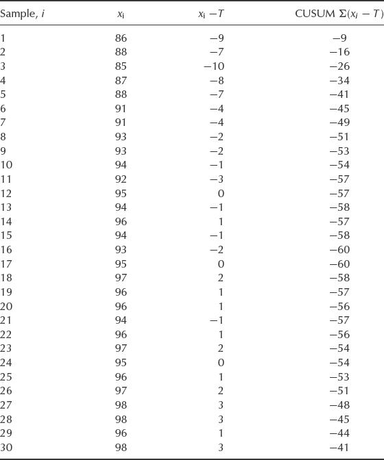
Table 13.4 shows data from a reliability test on a one-shot item. Batches of one hundred are tested, and the target success ratio is 0.95.

Figure 13.7 (a) shows the results plotted on a conventional run chart.

Figure 13.7 (b) shows the same data plotted on a CUSUM chart, with the CUSUM values calculated as shown in Table 13.4.

The CUSUM can be restarted with a new target value if a changed, presumably improved, process average is attained. Decisions on when to restart, the sample size to take, and scaling of the axes will depend upon particular circumstances.

Guidance on the use of CUSUM charts is given in British Standard BS 5703 (see Bibliography), and in good books on statistical process control, such as those listed in the Bibliography for Chapter 15.

Figure 13.7 (a) Run chart of data in Table 13.4. (b) CUSUM chart of data of Table 13.4.

13.10 Exploratory Data Analysis and Proportional Hazards Modelling

Exploratory data analysis is a simple graphical technique for searching for connections between time series data and explanatory factors. It is also used as an approach to analysing data for the purpose of formulating hypotheses worth testing. In the reliability context, the failure data are plotted as a time series chart, along with the other information. For example, overhaul intervals, seasonal changes, or different operating patterns can be shown on the chart. Figure 13.8 shows failure data plotted against time between scheduled overhauls. There is a clear pattern of clustering of failures shortly after each overhaul, indicating that the overhaul is actually adversely affecting reliability. In this case, further investigation would be necessary to determine the reasons for this, for example, the quality of the overhaul work might be inadequate. Another feature that shows up is a tendency for failures to occur in clusters of two or more. This seems to indicate that failures are often not diagnosed or repaired correctly the first time.

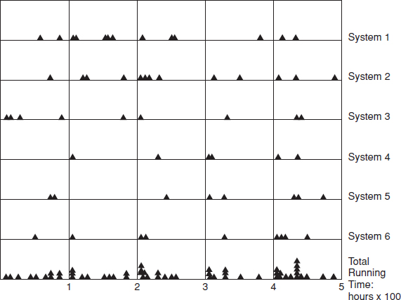
Figure 13.8 Time series chart: failure vs time (overhaul interval 1000 h).

This method of presenting data can be very useful for showing up causes of unreliability in systems such as vehicle fleets, process plant, and so on. The data can be shown separately for each item, or by category of user, and so on, depending on the situation, and analysed for connections or correlations between failures and the explanatory factors.

Proportional hazards modelling (PHM) is a mathematical extension of EDA. It is used to model the effect of secondary variables on product failures. The basic proportional hazards model is of the form

where λ(t Z₁, Z₂, . . ., Z_k) represents the hazard rate at time t, λ₀(t) is the baseline hazard rate function, Z₁, Z₂, . . ., Z_k are the explanatory factors (or covariates), and β₁, β₂, . . ., β_k are the model parameters.

In the proportional hazards model, the covariates are assumed to have multiplicative effects on the total hazard rate. In standard regression analysis or analysis of variance the effects are assumed to be additive. The multiplicative assumption is realistic, for example, when a system with several failure modes is subject to different stress levels, the stress having similar effects on most of the failure modes. The proportional hazards approach can be applied to failure data from repairable and non-repairable systems.

The theoretical basis of the method is described in Kalbfleisch and Prentice (2002). The derivation of the model parameters requires the use of advanced statistical software, as the analysis is based on iterative methods. This limits application of the technique to teams with specialist knowledge and access to the appropriate software.

13.11 Field and Warranty Data Analysis

Field returns and warranty data can be an excellent source for product reliability analysis and modelling. The field environment is the ultimate test for product performance; therefore the reliability should be evaluated based on field failures whenever possible. Warranty claims database can be a source of engineering analysis of the failure causes as well as for the forecasting of the future claims. However, working with warranty data requires an understanding of its specifics and limitations in order to produce meaningful results.

13.11.1 Field and Warranty Data Considerations

Warranty data comes in various shapes and forms depending on the industry, type of product, individual manufacturer, and many other factors. A typical warranty database contains a large amount of information about each claim, however a reliability practitioner should understand that besides ‘true’ failures there is a certain amount of ‘noise’ in this data.

Figure 13.9 shows an example of warranty database content. The ‘noise’ factors include NFFs (no fault found) common in the electronics industry (Chapter 9), fraudulent claims, inaccurate reporting including missing data and misuse. The amounts of ‘noisy’ claims would vary significantly based on the industry, type of the product and even individual manufacturer. Therefore it is important to be able to ‘clean’ the data distinguishing between the ‘relevant’ and ‘irrelevant’ claims and also further categorize them by failure modes. However, it is also important to remember that the product user is affected by all product failures regardless of their origin, therefore it is often beneficial to process the data ‘as is’ without removing those considered irrelevant.

Another complicating factor in high volume warranty analysis is that the items are continuously produced and sold; therefore warranty periods for different items begin at different times. Thus it is easier to model warranty in the product age format as opposed to the calendar time format.

It is also important for a reliability professional to remember that warranty periods are usually shorter than the expected life of a product, therefore warranty data does not normally provide enough information to evaluate the reliability at the later phases of product life, where wearout is expected.

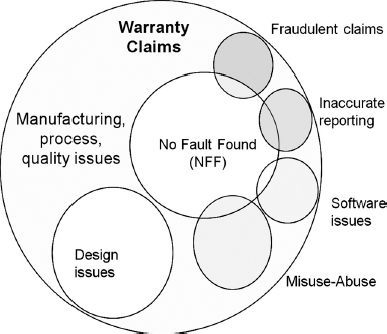
Figure 13.9 Warranty claims root causes.

13.11.2 Warranty Data Formats

Warranty databases often contain two types of data. One would have detailed information about each claim, while another type has the warranty statistics, such as sales volumes, number of failures and the relevant times to failure. These formats are covered below.

13.11.2.1 Individual Claims Data Format

Individual claims data contain various types of information about each failure. That usually includes the production date, sales date, failure date, description of the problem, location of the claim (country, state, region, etc.), cost of repair, who performed the repair, and so on. It may also contain the usage data, such as mileage, number of runs, cycles, loadings, and so on. Detailed claims data can be used for the engineering analysis and feedback on the root causes of design and manufacturing problems. Pareto charts Figure 13.1 can also be compiled after determining a root cause of each failure. Based on this information engineers can improve the existing product and also learn lessons to be incorporated in the design for reliability (DfR) process. For more engineering and business applications of warranty data analysis please see Kleyner (2010b). Individual claims data are often based on a sample, rather than on processing all of the returned items, especially if the number of repairs is large.

Individual claim analysis would also allow the analyst to separate the failure modes of interest and to enhance the statistical data analysis (see next section) by accounting for the failure modes of interest. For example if the individual claims analysis shows that 20% of all claims were caused by misdiagnosis or customer misuse, then we can accordingly adjust the statistics of the ‘true’ claims.

13.11.2.2 Statistical Data Format

Individual claims data is not sufficient for the life data analysis and forecasting. It needs to be combined with the information about the whole population of units in the field in order to be useful for a statistical analysis. Statistical warranty data (sometimes referred to as actuarial) typically contains the sales volumes, number of failed parts and the associated timing information, such as dates of manufacturing, sales, failure or repair.

In statistical data reporting it is often impractical to trace every individual item, especially in high volume production industries; therefore it is customary to group the data on a monthly or other predetermined time interval basis. The exact formats and the amount of information vary from industry to industry and even from company to company. One of the common data reporting formats is called MIS (Month in Service). It is widely used to track automotive warranties, but has been successfully applied in other industries.

Table 13.5 shows the example of warranty data in MIS format. For each month of sale (or month of production if warranty begins with shipping) the number of repaired or returned parts is recorded for each month in service. Other MIS information may include the financials, such as total warranty expenses for that month or the average cost per repair. Each sales month is tracked separately; however the totals can be calculated as weighted averages based on monthly volumes (bottom row of Table 13.5). Obviously the later the product has been manufactured (or sold) the fewer months of warranty claims will be recorded, affecting that month's contribution to the totals.

Another popular data format used by warranty professionals is called the ‘Nevada’ (the data table resembling the shape of American state of Nevada), which is also sometimes referred as the ‘Layer cake’. Table 13.6 shows the monthly returns from Table 13.5 presented in the Nevada format. The returns are shown in the calendar time format as opposed to the age format associated with MIS.

The Nevada format allows the user to convert shipping and warranty return data into the standard reliability data form of failures and suspensions so that it can easily be analysed with traditional life data analysis methods. At the end of the analysis period, all of the units that were shipped and have not failed in the time since shipment are considered to be suspensions. Commercially available warranty analysis software packages can handle various data entry formats. For example ReliaSoft Weibull++¯ has four different warranty data entry formats including the Nevada.

Table 13.5 Example of MIS (Month in Service) data (January – July 2011).

13.11.3 Warranty Data Processing

Most warranty claims result in repair or replacement of the failed part, therefore warranty data should be analysed using statistical analysis appropriate for the repairable systems, such as renewal process, non-homogeneous Poisson process (NHPP), and so on. Those are covered in Section 2.15, Section 6.7 and Section 13.8. This is especially true in the cases where devices are expected to experience repeat failures or undergo maintenance, such as operating machinery, plant equipment, airplanes, and so on. However in a large volume production of relatively simple parts the number of secondary failures is expected to be small. For example, the number of automotive electronics modules, which experienced secondary failures during warranty is typically below 5% or even 1% (see Kleyner and Sandborn, 2008) therefore applying non-repairable data analysis techniques would simplify the analysis and would not result in large calculation errors.

The cumulative failure function F(t) is easier to model than the renewal function or NHPP, therefore reliability R(t) can be obtained from life data analysis of warranty data. However since most units are expected to operate without failure through the warranty period, this data will be heavily censored with a large number of suspensions.

As shown in Figure 13.9, warranty data can be messy and often needs to be ‘cleaned’ before life data analysis can be performed. Another factor often complicating warranty data analysis is so-called ‘data maturation’. Warranty data is often limited to several months of observation, where the failure trend may not be established yet. Also there is often a lag between repair date and warranty system entry date, thus resulting in underreporting of the latest claims. All that may bias F(t) and the overall reliability data analysis. For more on warranty data collection and analysis see Blischke et al. (2011).

Table 13.6 Example of warranty data presented in the ‘Nevada’ (or the ‘Layer cake’) format.

Table 13.7 Cumulative percent failures for 6 months. Based on the data in Table 13.5.

Example 13.6

Estimate the product reliability at the 36-months warranty period based on the data presented in Table 13.5. Data in the bottom row of Table 13.5 can be used to calculate the cumulative failures (cdf) Table 13.7.

Two parameter Weibull distribution can be fit to the dataset in Table 13.7 using Weibull++¯, ‘Distribution Fit’ option in @Risk¯ or other distribution fitting software producing β = 1.11 and η = 297.9 months.

Therefore R(36 months) = exp(−(36/297.9)^1.11) = 90.8%

This forecast can only be considered tentative, since this data is based on just six months of observations. To make the matter worse, the sampled population was progressively decreasing with the number of months in service, which further decreases the accuracy of this warranty forecast. For example, Table 13.5 shows that the six-months’ warranty is only available for the January 2011 parts, while one month warranty data exists for all parts from January to May 2011. Furthermore, this data has not been filtered for the ‘irrelevant’ failures; therefore the design related reliability is expected to be somewhat higher than predicted.

More information on warranty data can be found in Blischke and Murthy (1996).

Questions

You can use life data analysis software to solve some of the problems below. If software is not available trial versions of Weibull++¯ and ALTA¯ can be downloaded from www.reliasoft.com.

1. Based on the existing data a reliability engineer has developed and implemented an accelerated test plan. Under the assumption of the exponential distribution a test provides MTTF = 300 hours. Given that the acceleration factor is 5.6, determine the reliability under normal conditions for a time equal to 200 hours.
2. Identify at least three models of stress-life relationships and provide examples when these might occur.
3. Consider the following data.
   1. Does the stress life relationship follow an expected log log relationship?

      Stress (V)	Time to fail (h)
      25	5.6
      50	10
      70	14.3
      90	27.8

   2. Give reasons why a log stress vs. log life relationship might not always be linear at high stress and at low stress.
4. Explain why a simple power law of life vs. stress is unlikely to apply to an assembly that consists of several different stressed components.
5. You desire to estimate the accelerating influences of a corrosive solution through an accelerated life test. The concentration of the solution will be the accelerating factor and four levels will be employed in the test. Metallic samples will be soaked in the various concentrations for 10% of the day and then allowed to air dry at room temperature. Describe how to approach this test and use the results in the future.
6. Let S measure the time-dependent strength of a material under test and S₀ is the initial strength as measured at the beginning of test. Prior tests and evaluations have suggested that the following stress time relationship appears to work.

   

   If the strength declines 20% after exactly three weeks of accelerated test, what is the expected time to failure at this condition, when the failure is defined as a decline of strength of 50%?

7. Let the functional relationship of question 6 become S⁴ = (S₀)⁴ − 4Ct instead (this is a typical degradation curve). Redo the analysis of question 6.
8. The following table of data was generated from a valid accelerated life test. The failure definition employed was the time to 10% failures of a sample operated at each condition. If the basic model below is correct, what are the values of the three unknowns E_o, N and B for the typical formula shown below?

   

   

9. Explain why the times between successive failures of a repairable system might not be independently and identically distributed (IID).
10. Question 3 in Chapter 3 describes the behaviour of a component in a ‘socket’ of a repairable system. Referring again to that question, suppose you have been given the additional information that machine B was put into service when machine A had accumulated 500 h, machine C when machine A had accumulated 1000 h, machine D when machine A had accumulated 1500 h, and machine E when machine A had accumulated 2000 h.
    1. Use this additional information about the sequencing of failures to calculate the trend statistic (Eq. 2.46), and hence judge whether, as far as this socket is concerned, the system is ‘happy’, ‘sad’ or indeterminate (IID) in terms of Figure 13.5.
    2. Repeat the exercise, but splitting the data to deal separately with (i) the first eight sequenced failures. and (ii) the second eight. What do these results tell you about the dangers of assuming IID failures when the assumption may not be valid?
11. Accelerated vibration test to failure has been performed on a sample of automotive radios. There were three G-levels of vibration referred here as 1-low, 2-medium, 3-high. What can be concluded from the Weibull plots for each stress level shown in Figure 13.10?

    

    Figure 13.10 Weibull charts of the test results.

12. Develop a test for a wind power generator to address corrosion caused by the combination of temperature and humidity. The generator will be installed at the climate conditions with humidity levels up to 80% RH (relative humidity). Generator is designed to operate 24 hours per day for 10 years. The field usage temperatures are distributed as follows: 20% of the time at 30 °C, 30% of the time at 20 °C and 10% of the time at 0 °C. Calculate the duration of the test at 85 °C-85% RH using Peck's model assuming E_A = 0.7eV and humidity power constant m = 3.0.
13. In an investigation into cracking of brake discs on a locomotive, a proportional hazards analysis was undertaken on a sample containing 205 failures and 905 censorings. (A failure was removal of an axle because a crack had propagated to such an extent that replacement was needed to avoid any possibility of fracture, a censoring was removal of an axle for any other reason.) Referring to Eqn (13.9), the covariates were:

    Z₁ = region of operation (0 for Eastern region, 1 for Western region).

    Z₂ = braking system (0 for type A, 1 for type B).

    Z₃ = disc material (0 for material X, 1 for material Y).

    The data were analysed using computer methods (the only practicable way) to give the following coefficients: β₁ = 0.39, β₂ = 0.72, β₃ = 0.95.

    1. At any given age, what is the ratio between the hazard functions of axles running on the two regions?
    2. What is the ratio for the two braking systems?
    3. What is the ratio for the two disc materials?

    [This example is based on real data first reported by Newton and Walley in 1983. The analysis is further developed in Bendell, Walley, Wightman and Wood (1986), ‘Proportional hazards modelling in reliability analysis – an application to brake disks on high-speed trains’, Quality and Reliability International, 2, 42–52.]

14. The following data give the times between successive failures of an aircraft air-conditioning unit: 48, 29, 502, 12, 70, 21, 29, 386, 59, 27, 153, 26 and 326 hours. When a unit fails it is repaired in situ. Repairs can be assumed to be instantaneous.
    1. Examine the distribution of failure times, treating the unit as a component on the aircraft.
    2. Examine the trend of failures, viewing the air- conditioning system itself as a repairable system.
    3. Describe clearly the conclusions to be drawn from both these analyses.
15. Two prototypes of a newly designed VHF communications set have been manufactured. Each has been subjected to a life-test as follows:

    Prototype A – had failures at 37, 53, 102, 230 and 480 h running; withdrawn from test at 600 h.

    Prototype B – started test when A was withdrawn (only one test rig was available) and had failures after 55, 290, 310, 780 and 1220 h; is still running, having accumulated 1700 h.

    1. On the assumption of random failures, estimate the failure rate and the probability of surviving a 100 h mission without failure.
    2. Revise your answers to (a) if you apply a reliability growth model to the data, assuming that all modifications found necessary during the test on prototype A were applied to prototype B.
16. Calculate the overall mean time between failures for the data in Question 10. Produce a CUSUM chart of the data, plotting Σ(t_i − T ) against i where t_i is the elapsed time between the ith and the (i − 1)th sequenced failures and T is the expected time since the previous failure based on the overall MTBF.

    From this plot, identifying when any change to the MTBF might have occurred, and estimate the MTBF before and after the change.

    Consider whether this plot shows the situation more clearly than a straightforward trend plot of cumulative failures against cumulative time.

17. Run the paperclip example as described at http://www.weibull.com/AccelTestWeb/paper_clip_example. htm Use the angle of bend as a stress variable and measure the fatigue life as a number of cycles till the clip's inner loop breaks. Run your own calculations and predict the fatigue life at 45 degree bend and check your results by actually running the experiment at 45 degree bend.
18. Vibration test has been conducted at two different stress levels: 4.0 and 6.0 G peak to peak acceleration. The results in cycles to failure are presented in the table below

    4.0 G Vibration	6.0 G Vibration
    9.60×105 cycles	4.92×104 cycles
    1.52×106 cycles	5.60×104 cycles
    8.35×105 cycles	5.32×104 cycles

    1. Determine the fatigue exponent b.
    2. Calculate the expected number of cycles to failure at the vibration level of 2.0G.
19. What are the purpose and the benefits of Pareto Analysis? Make the examples of the situations where using the Pareto Analysis would be beneficial.
20. A Pareto analysis of field return warranty data shows several categories which are approximately equal. In developing the corrective actions to reduce the number those problems how would you choose which of those categories to address first? Consider the criteria such as cost of fixing the problem, ease of fixing the problem, overall cost saving, cost-benefit analysis, how quick you will see the results and others.
21. Discuss the warranty claims root causes presented in Figure 13.9.
    1. Which of those categories are easiest to detect in a warranty database and which ones would be most difficult?
    2. How would be your course of actions in taking corrective actions for each category? Which ones would be easiest to take corrective action about and which would be most difficult?
    3. In your opinion, which categories would offer biggest cost savings?
22. What are the limitations of using acceleration models in developing accelerated test plans? Which limitations would be eliminated and which would remain if instead of using generic models we apply the models based on the actual accelerated test data?

Bibliography

Ascher, H. and Feingold, H. (1984) Repairable Systems Reliability, Dekker.

Blischke, W. and Murthy, D. (1996) Product Warranty Handbook, Marcel Dekker.

Blischke, W., Karim, R. and Murthy, D. (2011) Warranty Data Collection and Analysis, Springer.

British Standard BS 5703. Guide to Data Analysis and Quality Control using Cusum Techniques. British Standards Institute, London.

British Standard, BS 5760. Reliability of Systems, Equipments and Components, Part 2. British Standards Institution, London.

Clech, J-P., Henshall, G. and Miremadi, J. (2009) Closed-Form, Strain-Energy Based Acceleration Factors for Thermal Cycling of Lead-Free Assemblies. Proceedings of SMTA International Conference (SMTAI 2009), Oct. 4-8, 2009, San Diego, CA.

ISO IEC 60605. Equipment Reliability Testing. International Standards Organisation, Geneva.

JEDEC (2009) JEP122F Failure Mechanisms and Models for Semiconductor Devices. Published by JEDEC Association. Available at http://www.jedec.org/Catalog/catalog.cfm.

Kalbfleisch, J., Lawless, J. and Robinson, J. (1991), Methods for the Analysis and Prediction of Warranty Claims. Technometrics, 33(3) August.

Kalbfleisch, J. and Prentice, R. (2002) The Statistical Analysis of Failure Time Data, 2nd edn, Wiley.

Kleyner, A. (2010a) In the Twilight Zone of Humidity Testing. TEST Engineering & Management, August/September issue.

Kleyner A. (2010b) Discussion Warranted. Quality Progress, International Monthly Journal of American Society for Quality (ASQ). May 2010 issue, pp. 22–27.

Kleyner, A. and Sandborn, P. (2008) Minimizing life cycle cost by managing product reliability via validation plan and warranty return cost. International Journal of Production Economics, 112, 796–807.

Lawson, R. (1984) A review of the status of plastic encapsulated semiconductor component reliability. British Telecommunication Technology Journal, 2(2), 95–111.

Moltoft, J. (1994) Reliability Engineering Based on Field Information: The Way Ahead. Quality and Reliability Engineering International, 10, 399–409.

Nelson, W. (1989) Accelerated Testing: Statistical Models, Test Plans and Data Analysis, Wiley.

NIST (2006) Eyring. National Institute of Standards and Technology, online Handbook section 8.1.5.2 Available at: http://www.itl.nist.gov/div898/handbook/apr/section1/apr152.htm.

Norris, K. and Landzberg, A. (1969) Reliability of Controlled Collapse Interconnections. IBM Journal of Research and Development, 13(3), 266–271.

Ohring, M. (1998) Reliability and Failure of Electronic Materials and Devices, Academic Press.

Pan, N., Henshall, G.A., Billaut, F. et al. (2005) An Acceleration Model for Sn-Ag-Cu Solder Joint Reliability under Various Thermal Cycle Conditions, SMTA International, pp. 876–883.

Peck, D. (1986) Comprehensive Model for Humidity Testing Correlation. IEEE IRPS Proceedings, 44–50.

ReliaSoft (2010) Accelerated Life Testing Reference, ReliaSoft Publishing.

ReliaSoft (2010) ALTA-7 User's Guide, ReliaSoft Publishing.

ReliaSoft (2011) Accelerated Life Testing Reference. Online Reliability Engineering Resources. Available at http://www.weibull.com/acceltestwebcontents.htm.

Salmela, O. (2007) Acceleration Factors for Lead-Free Solder Materials. IEEE Transactions on Components and Packaging Technologies, 30(4), December 2007.

SEMATECH (2000) Semiconductor Device Reliability Failure Models. Technology Transfer # 00053955A-XFR. International SEMATECH Report. Available at: http://www.sematech.org/docubase/document/3955axfr.pdf.

Steinberg, D. (2000), Vibration Analysis for Electronic Equipment, 3rd edn, Wiley.

Steven E., Rigdon, S. and Basu, A. (2000) Statistical Methods for the Reliability of Repairable Systems, Wiley.

Trindade, D. and Nathan, S. (2005) Simple Plots for Monitoring the Field Reliability of Repairable Systems. Proceedings of the Annual Reliability and Maintainability Symposium (RAMS).

US MIL-HDBK-781. Reliability Testing for Equipment Development, Qualification and Production. Available from the National Technical Information Service, Springfield, Virginia.