
11
Design of Experiments and Analysis of Variance
11.1 Introduction
Product testing is a common part of reliability practitioner's work, which may also involve experimenting intended to improve the product design or some of its characteristics. This chapter deals with the problem of assessing the combined effects of multiple variables on a measurable output or other characteristic of a product, by means of experiments. When designs have to be optimized in relation to variations in parameter values, processes, and environmental conditions, particularly if these variations can have combined effects, we should use methods that can evaluate the effects of the simultaneous variations. For example, it might be necessary to maximize the power output from a generator, and minimize the variation of its output, in relationship to rotational speed, several dimensions, coil geometry, and load conditions. All of these could have single or combined effects which cannot all be easily or accurately computed using theoretical calculations.
Statistical methods of experimentation have been developed which enable the effects of variation to be evaluated in these types of situations. They are applicable whenever the effects cannot be easily theoretically evaluated, particularly when there is a large component of random variation or interactions between variables. For situations when multiple variables might affect an output, the methods are much more economical than performing separate experiments to evaluate the effect of one variable at a time. This ‘traditional’ approach also does not enable interactions to be analysed, when these are not known empirically. The rest of this chapter describes the statistical experimental methods, and how they can be adapted and applied to optimization and problem-solving in engineering.
11.2 Statistical Design of Experiments and Analysis of Variance
The statistical approach to design of experiments (DOE) and the analysis of variance (ANOVA) technique was developed by R. A. Fisher, and is a very elegant, economical and powerful method for determining the significant effects and interactions in multivariable situations. Analysis of variance is used widely in such fields as market research, optimization of chemical and metallurgical processes, agriculture and medical research. It can provide the insights necessary for optimizing product designs and for preventing and solving quality and reliability problems. Whilst the methods described below might appear tedious, there is a variety of commercially available software packages designed to analyse the results of statistical experiments. Minitab¯ is a widely utilized package, which will be used for illustration in this chapter.1
11.2.1 Analysis of Single Variables
The variance of a set of data (sample) is equal to

(Eq. 2.15), where n is the sample size and ![]() is the mean value. The population variance estimate is derived by dividing the sum of squares, Σ(xi −
is the mean value. The population variance estimate is derived by dividing the sum of squares, Σ(xi − ![]() )2, not by n but by (n − 1), where (n − 1) denotes the number of degrees of freedom (DF). Then
)2, not by n but by (n − 1), where (n − 1) denotes the number of degrees of freedom (DF). Then ![]() = Σ(xi −
= Σ(xi − ![]() )2/(n − 1) (Eq. 2.16).
)2/(n − 1) (Eq. 2.16).
Example 11.1
To show how the variance of a group of samples can be analysed, consider a simple experiment in which 20 bearings, five each from four different suppliers, are run to failure. Table 11.1 shows the results.
We need to know if the observed variation between the samples is statistically significant or is only a reflection of the variations of the populations from which the samples were drawn. Within each sample of five there are quite large variations. We must therefore analyse the difference between the ‘between sample’ (BS) and the ‘within sample’ (WS) variance and relate this to the populations.
The next step is to calculate the sample totals and sample means, as shown in Table 11.1. The overall average value
![]()
Since n is 20, the total number of degrees of freedom (DF) is 19. We then calculate the values of (xi − ![]() )2. These are shown in Table 11.2.
)2. These are shown in Table 11.2.
Table 11.1 Times to failure of 20 bearings.

Table 11.2 Values of (xi − ![]() )2 for the data of Table 11.1.
)2 for the data of Table 11.1.
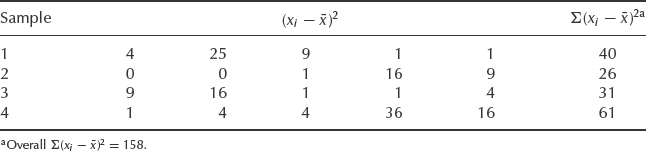
Table 11.3 Values of (xi − x′i) for the data of Table 11.1.
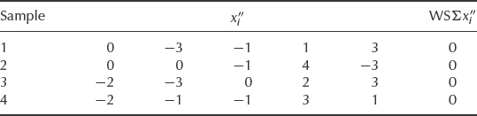
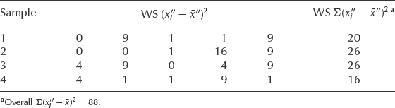
Table 11.4 Values of WS (![]() for the data of Table 11.1.
for the data of Table 11.1.
Having derived the total sum of squares and the DF, we must derive the WS and BS values. To derive the BS effect, we assume that each item value is equal to its sample mean (x′i). The sample means for each item in samples 1 to 4 are 4, 6, 5 and 9, respectively. The BS sums of squares (x′i − ![]() )2 are then, for each item in samples 1 to 4, 4, 0, 1 and 9, respectively, giving sample totals Σ(x′i −
)2 are then, for each item in samples 1 to 4, 4, 0, 1 and 9, respectively, giving sample totals Σ(x′i − ![]() )2 of 20, 0, 5 and 45 and an overall BS Σ(x′i −
)2 of 20, 0, 5 and 45 and an overall BS Σ(x′i − ![]() ) of 70. The BS DF is 4 – 1 = 3.
) of 70. The BS DF is 4 – 1 = 3.
Now we derive the equivalent values for the WS variance, by removing the BS effect. We achieve this by subtracting x′i from each item in the original table to give a value x″i. The result is shown in Table 11.3.
Table 11.4 gives the values of the WS sums of squares, derived by squaring the values as they stand, since now ![]() = 0. The number of WS DF is (5 − 1) × 4 = 16 (4 DF within each sample for a total of four samples). We can now tabulate the analysis of variance (Table 11.5).
= 0. The number of WS DF is (5 − 1) × 4 = 16 (4 DF within each sample for a total of four samples). We can now tabulate the analysis of variance (Table 11.5).
Table 11.5 Sources of variance for the data in Table 11.1.
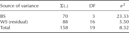
Table 11.6 Example 11.1 Minitab¯ solution.

If we can assume that the variables are normally distributed and that all the variances are equal, we can use the F-test (variance ratio test) (Section 2.12.4) to test the null hypothesis that the two variance estimates (BS and WS) are estimates of the same common (population) variance. The WS variance represents the experimental error, or residual variance. F is the ratio of the variances, and F-values for various significance levels and degrees of freedom are well tabulated and can easily be found on the Internet (see, e.g. NIST, 2011). F-values can also be calculated using Excel function FINV.
In this case
![]()
For 3 DF in the greater variance estimate and 16 DF in the smaller variance estimate, the 5% significance level of F is 3.239 = FINV(0.05, 3, 16). Since our value of F is greater than this, we conclude that the variance ratio is significant at the 5% level, and the null hypothesis that there is no difference between the samples is therefore rejected at this level.
A solution of Example 11.1 using the Minitab¯ software would provide additional analysis options, such as that shown in Table 11.6 and Figure 11.1.
In addition to the degrees of freedom, sums of squares, and variances already shown in Table 11.5 it calculates the F-value and its significance level (P-column). In this case it is 1-P = 1 – 0.022 = 0.978 which is greater than the sought significance of 95% .
Figure 11.1 gives a graphical representation of the data showing the mean values and their 95% confidence intervals. For example, it shows that 95% confidence bounds for sample 1 and sample 4 (column 1) do not overlap, graphically illustrating the statistical significance of that difference.
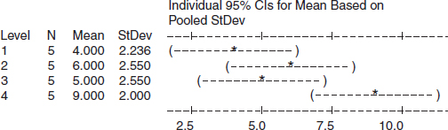
Figure 11.1 Minitab¯ chart showing statistically significant difference between samples 1 and 4.
11.2.2 Analysis of Multiple Variables (Factorial Experiments)
The method described above can be extended to analyse more than one source of variance. When there is more than one source of variance, interactions may occur between them, and the interactions may be more significant than the individual sources of variance. The following example will illustrate this for a three-factor situation.
Example 11.2
On a hydraulic system using ‘O’ ring seals, leaks occur apparently randomly. Three manufacturers' seals are used, and hydraulic oil pressure and temperature vary through the system. Argument rages as to whether the high temperature locations are the source of the problem, or the manufacturer, or even pressure. Life test data show that seal life may be assumed to be normally distributed at these stress levels, with variances which do not change with stress. A test rig is therefore designed to determine the effect on seal performance of oil temperature, oil pressure and type of seal. We set up the experiment in which we apply two values of pressure, 15 and 18 MN m−2 (denoted p1 and p2, in increasing order), and three values of temperature, 80, 100 and 120 °C (t1, t2 and t3, also in increasing order). We then select seals for application to the different test conditions, with two tests at each test combination. The results of the test are shown in Table 11.7, showing the elapsed time (h) to a detectable leak.
Table 11.7 Results of experiments on ‘O’ ring seals.

To simplify Table 11.7, subtract 100 from each value. The coded data then appear as in Table 11.8.
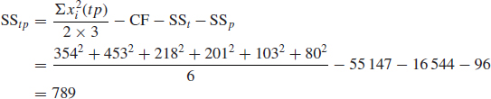
The sums of squares for the three sources of variation are then derived as follows:
- The correction factor:

Table 11.8 The data of Table 11.7 after subtracting 100 from each datum.

- The between types sum of squares:
Between three types there are two DF.
- The between pressures sum of squares:

Between two pressures there is one DF.
- The between temperatures sum of squares:

Between three temperatures there are two DF.
- The types–temperature interaction sum of squares:
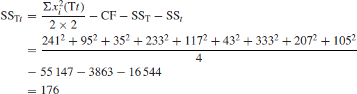
The T and the t effects each have 2 DF, so the interaction has 2 × 2 = 4 DF.
- The types–pressure interaction sum of squares:
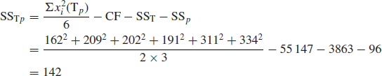
The T effect has 2 DF and the p effect has 1 DF, so the Tp interaction has 2 × 1 = 2 DF.
- The temperature–pressure interaction sum of squares:
The t effect has 2 DF and the p effect 1 DF. Therefore the tp interaction has 2 × 1 = 2 DF.
- The type–temperature–pressure interaction sum of squares:

There are 2 × 1 × 2 = 4 DF.
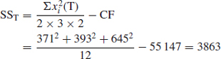
- The total sum of squares:

Total DF = 36 – 1 = 35 DF.
- Residual (experimental error) sum of squares is

The residual DF:
Total DF – (all other DF) = 35 -2 -1 -2 -4 -2 - 2 -4 = 18 DF
Examination of the analysis of variance table (Table 11.9) shows that all the interactions show variance estimates much less than the residual variance, and therefore they are clearly not statistically significant.
Having determined that none of the interactions are significant, we can assume that these variations are also due to the residual or experimental variance. We can therefore combine these sums of squares and degrees of freedom to provide a better estimate of the residual variance. The revised residual variance is thus:
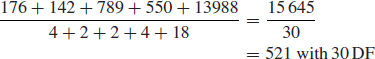
Table 11.9 Analysis of variance table.
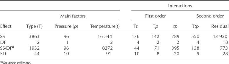
We can now test the significance of the main factors. Clearly the effect of pressure is not statistically significant. For the ‘type’ (T) main effect, the variance ratio F =1932/521 = 3.71 with 2 and 30 DF. Using Excel¯ function for F-distribution FDIST(3.71, 2, 30) = 0.0363, which shows that this is significant at the 5% level (3.63% ). For the temperature (t) main effect, F = 8272/521 = 15.88 with 2 and 30 DF. This is significant, even at the 1% level (FDIST(15.88, 2, 30) = 1.98 × 10⁻⁵).
Therefore the experiment shows that the life of the seals is significantly dependent upon operating temperature and upon type. Pressure and interactions show effects which, if important, are not discernible within the experimental error; the effects are ‘lost in the noise’. In other words, no type is significantly better or worse at higher pressures. Referring back to the original table of results, we can calculate the mean lives of the three types of seal, under the range of test conditions: type 1, 130 h; type 2, 132 h; and type 3, 154 h. Assuming that no other aspects such as cost predominate, we should therefore select type 3, which we should attempt to operate at low oil temperatures.
11.2.3 Non-Normally Distributed Variables
In Example 11.2 above it is important to note that the method described is statistically correct only for normally distributed variables. As shown in Chapter 2, in accordance with the central limit theorem many parameters in engineering are normally distributed. However, it is prudent to test variables for normality before performing an analysis of variance. If any of the key variables are substantially non-normally distributed, non-parametric analysis methods can be used, the data can be converted into normally distributed values, or other statistical methods can be applied. For more details on dealing with non-normal data see Deshpande (1995).
11.2.4 Two-Level Factorial Experiments
It is possible to simplify the analysis of variance method if we adopt a two-level factorial design for the experiment. In this approach, we take only two values for each main effect, high and low, denoted by + and −. Example 11.3 below shows the results of a three-factor non-replicated experiment (such an experiment is called a 23 factorial design, i.e. three factors, each at two levels).
Example 11.3
From the results of Table 11.10, the first three columns of Table 11.11 represent the design matrix of the factorial experiment. The response value is the mean of the values at each test combination or in this case, as there is no replication, the single test value.
Table 11.10 Results of a three-factor non-replicated experiment.
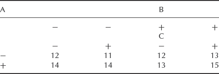
The main effects can be simply calculated by averaging the difference between the response values for each high and low factor setting, using the appropriate signs in the ‘factor’ columns. Thus:
![]()
Likewise,
![]()
and,
![]()
The sum of squares of each effect is then calculated using the formula
![]()
where k is the number of factors. Therefore,

Table 11.11 Response table and interaction of effects A, B, C.

Table 11.12 Analysis of variance table.

We can derive the interaction effects by expanding Table 11.11. Additional columns are added, one for each interaction. The signs under each interaction column are derived by algebraic multiplication of the signs of the constituent main effects. The ABC interaction signs are derived from AB × C or AC × B or BC × A.
The AB interaction is then
![]()
and
![]()
The other interaction sums of squares can be calculated in the same way and the analysis of variance table (Table 11.12) constructed.
To illustrate the additional capability of the software analysis, the quick analysis of the data in Example 11.3 with Minitab¯ would quickly produce the main effects diagram (Figure 11.2). Judging by the slopes of the lines we can easily notice the largest A main effect and lowest effect of ABC interaction.
Whilst the experiment in Example 11.3 indicates a large A main effect, and possibly an important BC interaction effect, it is not possible to test these statistically since no residual variance is available. To obtain a value of residual variance further replication would be necessary, or a value of experimental error might be available from other experiments. Alternatively, if the interactions, particularly high order interactions, are insignificant, they can be combined to give a residual value. Also, with so few degrees of freedom, the F test requires a very large value of the variance ratio in order to give high confidence that the effect is significant. Therefore, an unreplicated 23 factorial experiment may not always be sufficiently sensitive. However, the example will serve as an introduction to the next section, dealing with situations where several variables need to be considered.
11.2.5 Fractional Factorial Experiments
So far we have considered experiments in which all combinations of factors were tested, that is full factorial experiments. These can be expensive and time-consuming, since if the number of factors to be tested is f, the number of levels is L and the number of replications is r, then the number of tests to be performed is rL f, that is in the hydraulic seal example 2 × 32 = 18, or in a three-level four-factor experiment with two replications 2 × 34 = 162. In a fractional factorial experiment we economize by eliminating some test combinations. Obviously we then lose information, but if the experiment is planned so that only those effects and interactions which are already believed to be unimportant are eliminated, we can make a compromise between total information, or experiment costs, and experimental value.
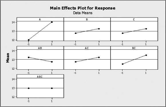
Figure 11.2 Main effects plots for Example 11.3 using Minitab¯.
A point to remember is that higher order interactions are unlikely to have any engineering meaning or to show statistical significance and therefore the full factorial experiment with several factors can give us information not all of which is meaningful.
We can design a fractional factorial experiment in different ways, depending on which effects and interactions we wish to analyse. Selection of the appropriate design is made starting from the full factorial design matrix. Table 11.13 gives the full design matrix for a 24 factorial experiment.
We select those interactions which we do not consider worth analysing. In the 24 experiment, for example, the ABCD interaction would not normally be considered statistically significant. We therefore omit all the rows in the table in which the ABCD column shows – Thus we eliminate half of our test combinations, leaving a half factorial experiment. What else do we lose as a result? Table 11.14 shows what is left of the experiment.
Examination of this table shows the following pairs of identical columns
A, BCD; B, ACD; C, ABD; D, ABC; AB, CD; AC, BD: AD, BC
This means that the A main effect and the BCD interaction effect will be indistinguishable in the results. In fact in any experiment to this design we will not be able to distinguish response values for these effects; we say that they are aliased or confounded. If we can assume that the first- and second-order interactions aliased in this case are insignificant, then this will be an appropriate fractional design, reducing the number of tests from 24 = 16 to ![]() × 24 = 8. We will still be able to analyse all the main effects, and up to three first-order interactions if we considered that they were likely to be significant. For example, if engineering knowledge tells us that the AB interaction is likely to be significant but the CD interaction not, we can attribute the variance estimate to the AB interaction.
× 24 = 8. We will still be able to analyse all the main effects, and up to three first-order interactions if we considered that they were likely to be significant. For example, if engineering knowledge tells us that the AB interaction is likely to be significant but the CD interaction not, we can attribute the variance estimate to the AB interaction.
Table 11.13 The full design matrix for a 24 factorial experiment.
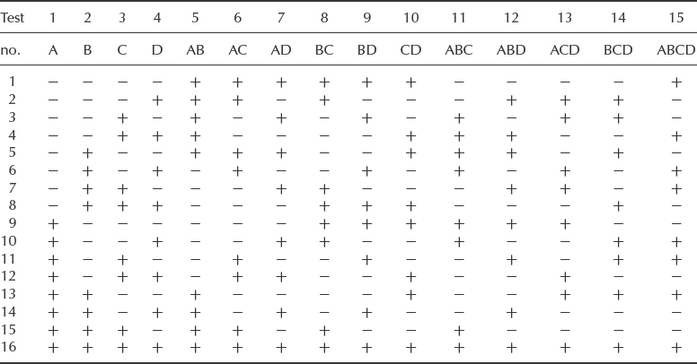
A similar breakdown of a 23 experiment would show that it is not possible to produce a fractional factorial without aliasing main effects with first-order interactions. This is unlikely to be acceptable, and fractional factorial designs are normally only used when there are four or more factors to be analysed. Quarter factorial designs can be used when appropriate, following similar logic to that described above. The value of using fractional factorial designs increases rapidly when large numbers of effects must be analysed. For example, if there are seven main effects, a full factorial experiment would analyse a large number of high level interactions which would not be meaningful, and would require 27 = 128 tests for no repeats. We can design a sixteenth fractional factorial layout with only eight tests, which will analyse all the main effects and most of the first-order interactions, as shown in Table 11.15. The aliases are deliberately planned, for example by evaluating the signs for the D column by multiplying the signs for A and B, and so on. We can select which interactions to alias by engineering judgement. It should be noted that other effects are also aliased. The full list of aliased effects can be derived by multiplying the aliased effects. For example, if D and AB are aliased, then the ABD interaction effect is also aliased, and so on. (If a squared term arises, let the squared term equal unity, e.g. AB × AC = A2 BC = BC.)
Table 11.14 Table 11.13 omitting rows where ABCD gives minus.

Table 11.15 Sixteenth fractional factorial layout for seven main effects.

There are various methods of constructing fractional factorial experiments to reduce the number of factors and combinations. Detailed coverage of those techniques is beyond the scope of this chapter, therefore for more information refer to Hinkelmann and Kempthorne (2008), Mathews (2005) or other references at the end of this chapter.
11.3 Randomizing the Data
At this stage it is necessary to point out an essential aspect of any statistically designed experiment. Significant sources of variance must be made to show their presence not only against the background of experimental error but against other sources of variation which might exist but which might not be tested for in the experiment. For instance, in Example 11.2, a source of variation might be the order in which seals are tested, or the batch from which seals are drawn. To eliminate the effects of extraneous factors and to ensure that only the effects being analysed will affect the results, it is important that the experiment is randomized. Thus the items selected for test and the sequence of tests must be selected at random, using random number tables or another suitable randomizing process. In Example 11.2, test samples should have been drawn at random from several batches of seals of each type and the test sequences should also have been randomized. It is also very important to eliminate human bias from the experiment, by hiding the identity of the items under test, if practicable.
If the items under test undergo a sequence of processes, for example heat treatment, followed by machining, then plating, the items should undergo each process in random order, that is separately randomized for each process.
Because of the importance of randomizing the data, it is nearly always necessary to design and plan an experiment to provide the data for analysis of variance. Data collected from a process as it normally occurs is unlikely to be valid for this purpose. Careful planning is important, so that once the experiment starts unforeseen circumstances do not cause disruption of the plan or introduce unwanted sources of variation or bias. A dummy run can be useful to confirm that the experiment can be run as planned.
11.4 Engineering Interpretation of Results
A statistical experiment can always, by its nature, produce results which conflict with the physical or chemical basis of the situation. The probability of a variance estimate being statistically significant in relation to the experimental error is determined in the analysis, but we must always be on the lookout for the occurrence of chance results which do not fit our knowledge of the processes being studied. For example, in the hydraulic seal experiment we could study further the temperature–pressure interaction. Since the variance estimate for this interaction was higher than for the other interactions we might be tempted to suspect some interaction. In another experiment the seals might be selected in such a way that this variance estimate showed significance.

Figure 11.3 Temperature–pressure interactions.
Figure 11.3 shows the interaction graphically, in two forms. If there were no interaction, that is the two effects acted quite independently upon seal life, the lines would be parallel between t1t2, t2t3 or p1p2. In this case an interaction appears to exist between 80(t1) and 100 °C(t2), but not between 100 and 120 °C(t3). This we can dismiss as being unlikely, taking into account the nature of the seals and the range of pressures and temperatures applied. That is not to say that such an interaction would always be dismissed, only that we can legitimately use our engineering knowledge to help interpret the results of a statistical experiment. The right balance must always be struck between the statistical and engineering interpretations. If a result appears highly significant, such as the temperature main effect, then it is conversely highly unlikely that it is a perverse result. If the engineering interpretation clashes with the statistical result and the decision to be made based on the result is important, then it is wise to repeat the experiment, varying the plan to emphasize the effects in question. In the hydraulic seal experiment, for example, we might perform another experiment, using type 3 seals only, but at three values of pressure as well as three values of temperature, and making four replications of each test instead of only two.
11.5 The Taguchi Method
Genichi Taguchi (1986), developed a framework for statistical design of experiments adapted to the particular requirements of engineering design. Taguchi suggested that the design process consists of three phases: system design, parameter design and tolerance design. In the system design phase the basic concept is decided, using theoretical knowledge and experience to calculate the basic parameter values to provide the performance required. Parameter design involves refining the values so that the performance is optimized in relation to factors and variation which are not under the effective control of the designer, so that the design is ‘robust’ in relation to these. Tolerance design is the final stage, in which the effects of random variation of manufacturing processes and environments are evaluated, to determine whether the design of the product and the production processes can be further optimized, particularly in relation to cost of the product and the production processes. Note that the design process is considered to explicitly include the design of the production methods and their control. Parameter and tolerance design are based on statistical design of experiments.
Taguchi separates variables into two types. Control factors are those variables which can be practically and economically controlled, such as a controllable dimensional or electrical parameter. Noise factors are the variables which are difficult or expensive to control in practice, though they can be controlled in an experiment, for example ambient temperature, or parameter variation within a tolerance range. The objective is then to determine the combination of control factor settings (design and process variables) which will make the product have the maximum ‘robustness’ to the expected variation in the noise factors. The measure of robustness is the signal-to-noise ratio, which is analogous to the term as used in control engineering.
Figure 11.4 illustrates the approach. This shows the response of an output parameter to a variable. This could be the operating characteristic of a transistor or of a hydraulic valve, for example. If the desired output parameter value is A, setting the input parameter at A', with the tolerance shown, will result in an output centred on A, with variation as shown. However, the design would be much better, that is more robust to variation of the input parameter, if this were centred at B', since the output would be much less variable with the same variation of the input parameter. The fact that the output value is now too high can be adjusted by adding another component to the system, with a linear or other less sensitive form of operating characteristic. This is a simple case for illustration, involving only one variable and its effect. For a multi-dimensional picture, with relationships which are not known empirically, the statistical experimental approach must be used.
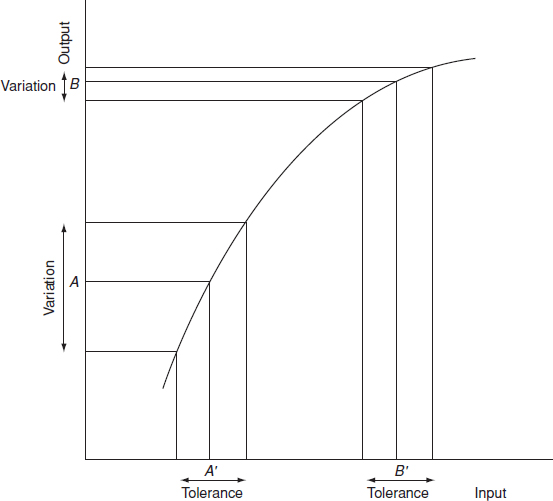
Figure 11.4 Taguchi method (1).

Figure 11.5 Taguchi method (2).
Figure 11.5 illustrates the concept when multiple variations, control and noise factors affect the output of interest. This shows the design as a control system, whose performance must be optimized in relation to the effect of all variations and interactions.
The experimental framework is as described earlier, using fractional factorial designs. Taguchi argued that, in most engineering situations, interactions do not have significant effects, so that much reduced, and therefore more economical, fractional factorial designs can be applied. When necessary, subsidiary or confirmatory experiments can be run to ensure that this assumption is correct. Taguchi developed a range of such design matrices, or orthogonal arrays, from which the appropriate one for a particular experiment can be selected. For example, the ‘L8’ array is a sixteenth fractional factorial design for seven variables, each at two levels, as shown in Table 11.14. (The ‘L’ refers to the Latin square derivation.) Further orthogonal arrays are given in Taguchi (1986), Ross (1988), Condra (1993) and Roy (2001).
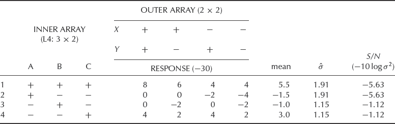
The arrays can be combined, to give an inner and an outer array, as shown in Table 11.16. The inner array contains the control factors, and the outer array the noise factors. The signal-to-noise ratio is calculated for the combination of control factors being considered, using the outer array, the formula depending on whether the desired output parameter must be maximized, minimized or centralized. The expressions are as follows:
Table 11.16 Results of Taguchi experiment on fuel system components (Example 11.4).
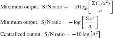
where x is the mean response for the range of control factor settings, and ![]() is the estimate of the standard deviation. The ANOVA is performed as described earlier, using the S/N ratio calculated for each row of the inner array. The ANOVA can, of course, also be performed on the raw response data.
is the estimate of the standard deviation. The ANOVA is performed as described earlier, using the S/N ratio calculated for each row of the inner array. The ANOVA can, of course, also be performed on the raw response data.
Example 11.4
Table 11.16 shows the results of a Taguchi experiment on a fuel control system, with only the variation in components A, B and C being considered to be significant. These are then selected as control factors (Inner array). The effects of two noise factors, X and Y, (Outer Array) are to be investigated. The design must be robust in terms of the central value of the output parameter, fuel flow, that is minimal variation about the nominal value.
Figure 11.6 shows graphically the effects of varying the control factors on the mean response and signal-to-noise ratio. Variation of C has the largest effect on the mean response, with A and B also having effects. However, variation of B and C has negligible effects on the signal-to-noise ratio, but the low value of A provides a much more robust design than the higher value.
This is a rather simple experimental design, to illustrate the principles. Typical experiments might utilize rather larger arrays for both the control and noise factors. Most commercially available software packages include the Taguchi method as one of the DOE options.

Figure 11.6 Results of Taguchi experiment (Example 11.4).
11.6 Conclusions
Statistical experimental methods of design optimization and problem-solving in engineering design and production can be very effective and economic. They can provide higher levels of optimization and better understanding of the effects of variables than is possible with purely deterministic approaches, when the effects are difficult to calculate or are caused by interactions. However, as with any statistical method, they do not by themselves explain why a result occurs. A scientific or engineering explanation must always be developed, so that the effects can be understood and controlled.
It is essential that careful plans are made to ensure that the experiments will provide the answers required. This is particularly important for statistical experiments, owing to the fact that several trials are involved in each experiment, and this can lead to high costs. Therefore a balance must be struck between the cost of the experiment and the value to be obtained, and care must be taken to select the experiment and parameter ranges that will give the most information. The ‘brainstorming’ approach is associated with the Taguchi method, but should be used in the planning of any engineering experiment. In this approach, all involved in the design of the product and its production processes meet and suggest which are the likely important control and noise factors, and plan the experimental framework. The team must consider all sources of variation, deterministic, functional and random, and their likely ranges, so that the most appropriate and cost-effective experiment is planned. A person who is skilled and experienced in the design and analysis of statistical experiments must be a team member, and may be the leader. It is important to create an atmosphere of trust and teamwork, and the whole team must agree with the plan once it is evolved. Note the similarity with the Quality Function Deployment method described in Chapter 7. The philosophical and psychological basis is the same, and QFD should highlight the features for which statistical experiments should be performed.
Statistical experiments are equally effective for problem solving. In particular, the brainstorming approach very often leads to the identification and solution of problems even before experiments are conducted, especially when the variation is functional, as described earlier.
The results of statistical experiments should be used as the basis for setting the relevant process controls for production. This aspect is covered in Chapter 15. In particular, the Taguchi method is compatible with modern concepts of statistical process control in production, as described in Chapter 15, as it points the way to minimizing the variation of responses, rather than just optimizing the mean value. The explicit treatment of control and noise factors is an effective way of achieving this, and is a realistic approach for most engineering applications.
The Taguchi approach has been criticized by some of the statistics community and by others (see, e.g. Logothetis, 1990 and Ryan, 2001), for not being statistically rigorous and for under-emphasizing the effects of interactions. Whilst there is some justification for these criticisms, it is important to appreciate that Taguchi has developed an operational method which deliberately economizes on the number of trials to be performed, in order to reduce experiment costs. The planning must take account of the extent to which theoretical and other knowledge, for example experience, can be used to generate a more cost-effective experiment. For example, theory and experience can often indicate when interactions are unlikely or insignificant. Also, full randomization of treatments might be omitted in an experiment involving different processing treatments, to save time. Taguchi recommends that confirmatory experiments should be conducted, to ensure that the assumptions made in the plan are valid.
It is arguable that Taguchi's greatest contribution has been to foster a much wider awareness of the power of statistical experiments for product and process design optimization and problem solving. The other major benefit has been the emphasis of the need for an integrated approach to the design of the product and of the production processes.
Statistical experiments can be conducted using computer-aided design software, when the software includes the necessary facilities, such as Monte Carlo simulation and statistical analysis routines. Of course there would be limitations in relation to the extent to which the software truly simulates the system and its responses to variation, but on the other hand experiments will be much less expensive, and quicker, than using hardware. Therefore initial optimization can often usefully be performed by simulation, with hardware experiments being run to confirm and refine the results.
The methods described in this chapter are appropriate for analysing cause-and-effect relationships which are linear, or which can be considered to be approximately linear over the likely range of variation. They cannot, of course, be used to analyse non-linear or discontinuous functions, such as resonances or changes of state.
The correct approach to the use of statistical experiments in engineering design and development, and for problem solving, is to use the power of all the methods available, as well as the skills and experience of the people involved. Teamwork and training are essential, and this in turn implies good management.
Questions
You can use statistical software to solve some of the problems below. If software is not available, trial versions of Minitab¯ or ReliaSoft DOE++¯ can be downloaded from www.minitab.com or www.reliasoft.com respectively.
- A manufacturer has undertaken experiments to improve the hot-starting reliability of an engine. There were two control factors, mixture setting (M) and ignition timing (T), which were each set at three levels. The trials were numbered as below (which is a full factorial, equivalent to a Taguchi L9 orthogonal array with only two of its four columns allocated):

The response variable was the number of starter-motor shaft revolutions required to start the engine. Twenty results were obtained at each setting of the control factors, with averages as follows:

- What initial conclusions can be drawn about the control factors and their interaction (without performing a significance test)?
- There are two identifiable noise factors (throttle position and clutch pedal position), both of which can be set at two levels. How would the noise factors have been incorporated into the experimental design?
- Do you think a Taguchi signal-to-noise ratio would be a better measure than the average revs? Which one would you use?
- What additional information do you need to perform an analysis of variance?
-
- It has been suggested that reliability testing should not be applied to proving a single design parameter but should instead be based on simple factorial experimentation on key factors which might improve reliability. What do you think of this idea?
- The following factors have been suggested as possible influences on the reliability of an electromechanical assembly:
- electrical terminations (wrapped or soldered).
- type of switching circuit (relay or solid-state).
- component supplier (supplier 1 or supplier 2).
- cooling (convection or fan).
It is suspected that D might interact with B and C.
An accelerated testing procedure has been developed whereby assemblies are subjected to repeated environmental and operational cycles until they fail. As this testing is expensive, a maximum of 10 prototypes can be made and tested. Design a suitable experiment, and identify all aliased interactions.
- One measure of the reliability of a portable communications receiver is its ability to give adequate reception under varying signal strengths, which are strongly influenced by climatic conditions and other environmental factors outside the user's control. It was decided that, within the design of a receiver, there were seven factors which could possibly influence the quality of reception.
An experiment was designed using a 27−3 layout. In the design shown in Table 11.13, the six factors (denoted A–G), each at two levels, were allocated respectively to columns 1, 2, 3, 4, 12, 14 and 15. The remaining columns were left free for evaluation of interactions. It was felt safe to assume that three- and four-factor interactions would not occur.
In the experiment the 16 prototype receivers were installed in an area of known poor reception, and each was evaluated for performance on four separate occasions (between which the environmental conditions varied in a typical manner). The results are shown below (the response being an index of reception quality):
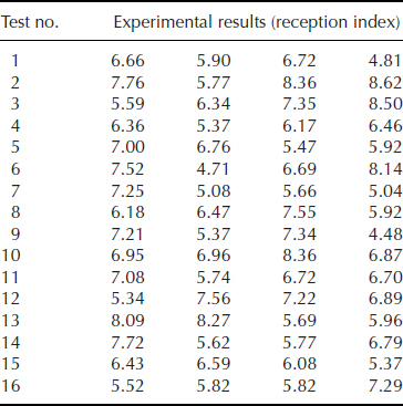
Calculate the maximum output (‘biggest is best’) signal-to-noise ratios. From these, calculate the effects and sums of squares for signal-to-noise for all the factors and interactions, and carry out an analysis of variance using these values to test the significance of the various factors and interactions. What would you recommend as the final design?
- When would you use Taguchi in place of DOE to evaluate contributors to a response? Explain.
- Why should we always Dry-Run the DOE or Taguchi set-up before performing the experiment? Explain.
- Why is it important to randomize for a DOE? Explain.
- How does DOF (degrees of freedom) within the experiment help to determine significance? Explain.
- You are conducting the experiments with two different types of solder alloys (Alloy A and Alloy B) and different temperature excursion during thermal cycling. The results of these experiments are presented in the Table in form of MTTF.

Analyse the data and determine which factors are significant.
Generate the main effect plots.
Derive the equation linking MTTF with the test variables. Consider the main effects as well as the interactions.
Run ANOVA on the same data and compare the results.
Bibliography
Bhote, K.R. (1988) World Class Quality, American Management Association.
Box, G.E., Hunter, W.G. and Hunter, J.S. (1978) Statistics for Experimenters, Wiley.
Breyfogle, F. (1992) Statistical Methods for Testing, Development and Manufacturing, Wiley-Interscience.
Condra, L. (1993) Reliability Improvement with Design of Experiments, Marcel Dekker.
Deshpande, J., Gore, A. and Shanubhogue, A. (1995) Statistical Analysis of Nonnormal Data, Wiley.
Grove, D. and Davis, T. (1992) Engineering Quality and Design of Experiments, Longman Higher Education.
Hinkelmann, K. and Kempthorne, O. (2008) Design and Analysis of Experiments, Introduction to Experimental Design, Wiley Series in Probability and Statistics.
Lipson, C. and Sheth, N.J. (1973) Statistical Design and Analysis of Engineering Experiments, McGraw-Hill.
Logothetis, N. and Wynn, H. (1990) Quality through Design, Oxford University Press.
Mason, R.L., Gunst R.F. and Hess J.L. (1989) Statistical Design and Analysis of Experiments, Wiley.
Mathews, P. (2005) Design of Experiments with MINITAB, American Society for Quality (ASQ) Press.
Montgomery, D. (2000) Design and Analysis of Experiments, 5th edn, Wiley.
NIST (2011) Section 1.3.6.7.3 Upper Critical Values of the F-Distribution. Engineering Statistics Handbook, published by NIST. Available at: http://www.itl.nist.gov/div898/handbook/eda/section3/eda3673.htm.
Park, S. (1996) Robust Design and Analysis for Quality Engineering, Chapman & Hall.
Ross, P.J. (1988) Taguchi Techniques for Quality Engineering, McGraw-Hill.
Roy, R. (2001) Design of Experiments Using the Taguchi Approach, Wiley-Interscience.
Ryan, T. (2001) Statistical Methods for Quality Improvement, 2nd edn, Wiley-Interscience.
Taguchi, G. (1986) Introduction to Quality Engineering, Unipub/Asian Productivity Association.
Taguchi, G. (1978). Systems of Experimental Design, Unipub/Asian Productivity Association.
1 Portions of the input and output contained in this publication/book are printed with permission of Minitab Inc. All material remains the exclusive property and copyright of Minitab Inc. All rights reserved.