2.1 Classical Current Control Methods

One of the most studied topics in power converters control is current control, for which there are two classical control methods that have been extensively studied over the last few decades: namely, hysteresis control and linear control using pulse width modulation (PWM) [4, 1, 2].

2.1.1 Hysteresis Current Control

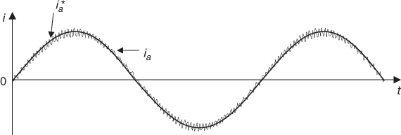
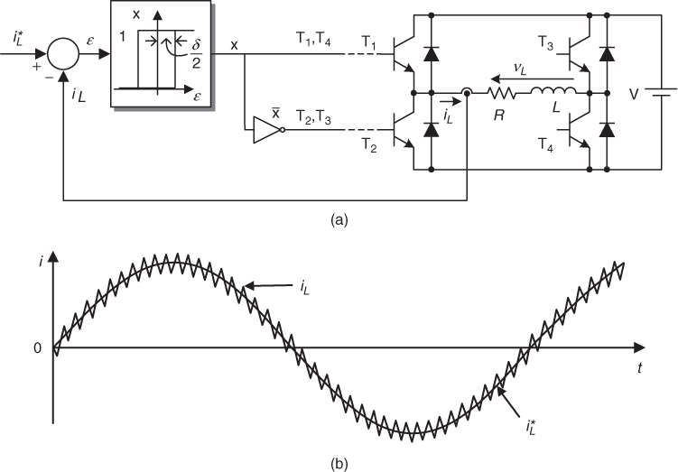
The basic idea of hysteresis current control is to keep the current inside the hysteresis band by changing the switching state of the converter each time the current reaches the boundary. Figure 2.1 shows the hysteresis control scheme for a single-phase inverter. Here, the current error is used as the input of the comparator and if the current error is higher than the upper limit δ/2, the power switches T₁, T₄ are turned on and T₂, T₃ are turned off. The opposite switching states are generated if the error is lower than − δ/2. It can be observed in Figure 2.1 that with this very simple strategy the load current i_L follows the waveform of the reference current very well, which in this case is sinusoidal.

Figure 2.1 Hysteresis current control for a single-phase inverter. (a) Control scheme. (b) Load current

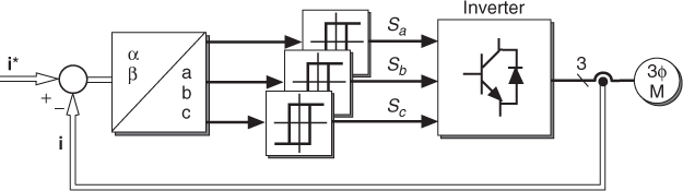
For a three-phase inverter, measured load currents of each phase are compared to the corresponding references using hysteresis comparators, as shown in Figure 2.2. Each comparator determines the switching state of the respective inverter leg (S_a, S_b, and S_c) such that the load currents are forced to remain within the hysteresis band. Due to the interaction between the phases, the current error is not strictly limited to the value of the hysteresis band. A simplified diagram of this control strategy is shown in Figure 2.3.

Figure 2.2 Hysteresis current control for a three-phase inverter

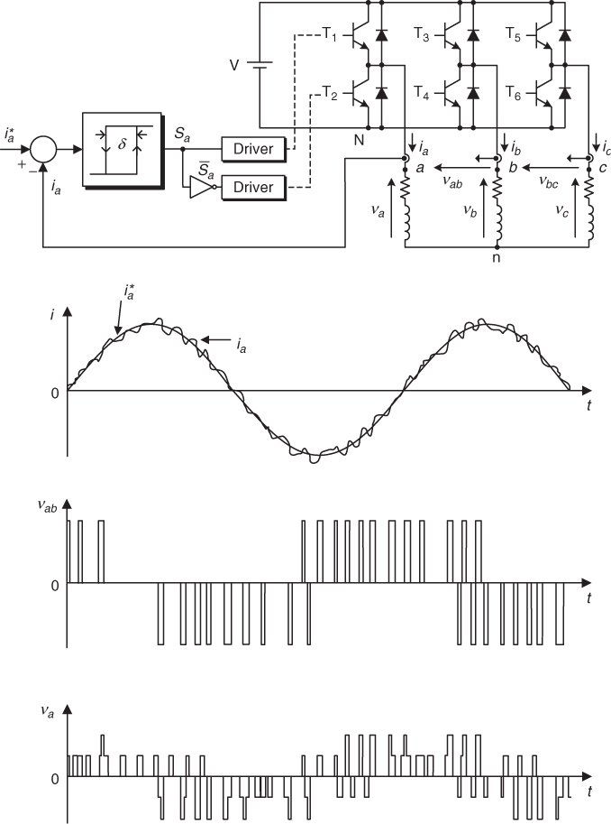
Figure 2.3 Three-phase hysteresis current control scheme

This method is conceptually simple and the implementation does not require complex circuits or processors. The performance of the hysteresis controller is good, with a fast dynamic response. The switching frequency changes according to variations in the hysteresis width, load parameters, and operating conditions. This is one of the major drawbacks of hysteresis control, since variable switching frequency can cause resonance problems. In addition, the switching losses restrict the application of hysteresis control to lower power levels [4]. Several modifications have been proposed in order to control the switching frequency of the hysteresis controller.

When implemented in a digital control platform, a very high sampling frequency is required in order to keep the controlled variables within the hysteresis band all the time.

2.1.2 Linear Control with Pulse Width Modulation or Space Vector Modulation

Considering a modulator stage for the generation of control signals for the power switches of the converter allows one to linearize the nonlinear converter. In this way, any linear controller can be used, the most common choice being the use of proportional–integral (PI) controllers.

2.1.2.1 Pulse Width Modulation

In a pulse width modulator, the reference voltage is compared to a triangular carrier signal and the output of the comparator is used to drive the inverter switches. The application of a pulse width modulator in a single-phase inverter is shown in Figure 2.4. A sinusoidal reference voltage is compared to the triangular carrier signal generating a pulsed voltage waveform at the output of the inverter. The fundamental component of this voltage is proportional to the reference voltage.

Figure 2.4 Pulse width modulator for a single-phase inverter

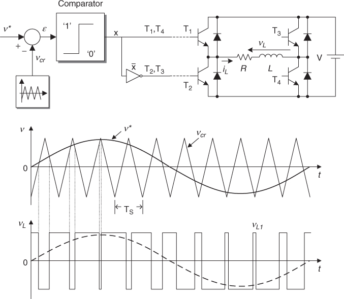
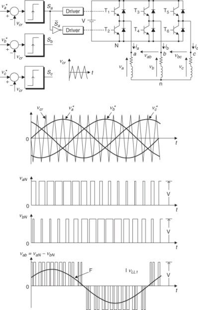
In a three-phase inverter, the reference voltage of each phase is compared to the triangular waveform, generating the switching states for each corresponding inverter leg, as shown in Figure 2.5. Output voltages for phases a and b, v_aN and v_bN, and line-to-line voltage v_ab are also shown in this figure.

Figure 2.5 Pulse width modulator for a three-phase inverter

2.1.2.2 Linear Control with Space Vector Modulation

A variation of PWM is called space vector modulation (SVM), in which the application times of the voltage vectors of the converter are calculated from the reference vector. It is based on the vectorial representation of the three-phase voltages, defined as

2.1

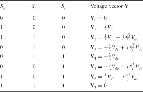
where v_aN, v_bN, and v_cN are the phase-to-neutral (N) voltages of the inverter and a = e^j2[π]/3. The output voltages of the inverter depend on the switching state of each phase and the DC link voltage, v_xN = S_xV_dc, with x = {a, b, c}. Then, taking into account the combinations of the switching states of each phase, the three-phase inverter generates the voltage vectors listed in Table 2.1 and depicted in Figure 2.6

Figure 2.6 Principles of space vector modulation (SVM). (a) Voltage vectors and sector definition. (b) Generation of the reference vector in a generic sector

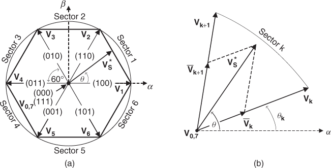
Table 2.1 Switching states and voltage vectors

.

Considering the voltage vectors generated by the inverter, the α − β plane is divided into six sectors, as shown in Figure 2.6. In this way, a given reference voltage vector v^*, located at a generic sector k, can be synthesized using the adjacent vectors V_k, V_k+1, and V₀, applied during t_k, t_k+1, and t₀, respectively. This can be summarized with the following equations:

2.2

2.3

where T is the carrier period and t_k/T, t_k+1/T, and t₀/T are the duty cycles of their respective vectors. Using trigonometric relations the application time for each vector can be calculated, resulting in

2.4

2.5

2.6

where θ is the angle of the reference vector v^* and θ_k is the angle of vector V_k.

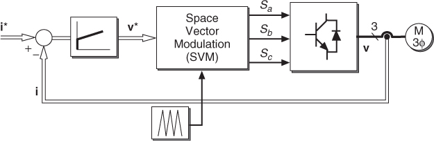
A classical current control scheme using SVM is shown in Figure 2.7. Here, the error between the reference and the measured load current is processed by a PI controller to generate the reference load voltages.

Figure 2.7 Classical control scheme using SVM

With this method, constant switching frequency, fixed by the carrier, is obtained. The performance of this control scheme depends on the design of the controller parameters and on the frequency of the reference current. Although the PI controller assures zero steady state error for continuous reference, it can present a noticeable error for sinusoidal references. This error increases with the frequency of the reference current and may become unacceptable for certain applications [4]. To overcome the problem of the PI controller with sinusoidal references, the standard solution is to modify the original scheme considering a coordinate transformation to a rotating reference frame in which the reference currents are constant values.

Figure 2.8 shows the waveform of the load current in one phase of the inverter generated using the control scheme of Figure 2.7.

Figure 2.8 Load current for a classical control scheme using SVM