10.4 Hard Constraints

One of the advantages of predictive control is the possibility of achieving direct control of the output variables without the need for inner control loops. However, it can be found in several cases that as the internal variables are not controlled, they can reach values that are outside their allowed range. In a traditional cascaded control scheme, this kind of limitation of the internal variables is considered by including saturation levels for the references of these variables. In a predictive control scheme, these limitations can be included as an additional term in the cost function.

As an example, the predictive torque control explained in Chapter 8 will be considered. In this control scheme, the electrical torque T_e and the stator flux magnitude are directly controlled using the following cost function [7]:

10.21

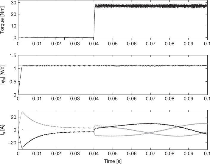
Here, the stator currents are not directly controlled and at steady state they are sinusoidal and their magnitude is within the allowed limits. However, during some transients these currents can be very high, damaging the inverter or the machine. The startup of the induction machine using this control scheme is shown in Figure 10.7. It can be seen in this figure that during the initial transient the stator currents can be considerably higher than the currents at full torque. It is desirable to consider the limitation of these currents in the predictive control scheme.

Figure 10.7 Predictive torque and flux control. Torque, stator flux magnitude, and stator currents at startup (Miranda et al., 2009 © IEEE)

Taking into account the idea of predictive control, the optimization algorithm must discard any switching state that makes the predicted currents exceed the predefined limit, and from those that do not violate the limits select the one that minimizes the torque and flux error. This procedure can be implemented as an additional nonlinear term in the cost function that generates a very high value when the currents exceed the allowed limits, and is equal to zero when the currents are within the limits. The resulting cost function is

10.22

where is the predicted stator current vector, is a nonlinear function defined as

10.23

and i_max is the value of the maximum allowed stator current magnitude.

The effect of this additional term in the cost function can be observed in Figure 10.8 for the same startup conditions as in Figure 10.7. It can also be seen that the stator current magnitude is saturated at the defined limit i_max = 15 A. The operation of the predictive control when the stator currents are below the limits is identical for both cases.

Figure 10.8 Predictive torque and flux control. Torque, stator flux magnitude, and stator currents at startup with stator current limitation (Miranda et al., 2009 © IEEE)

Another example of current limitation can be found in Chapter 9 for a permanent magnet synchronous motor.

The same idea of using a nonlinear function like the one presented in this section can be used to limit any variable in any predictive control scheme.