11.4 Examples

11.4.1 Switching Frequency Reduction

A predictive current control scheme with reduction of the switching frequency for a NPC inverter was presented in Chapter 5. In this scheme, the cost function presents a primary term for current reference tracking and a secondary term for reduction of the switching frequency:

11.2

The secondary term corresponds to the predicted number of switchings involved when changing from the present to the future switching state. Thus by increasing the associated weighting factor λ_sw it is expected that this term gains more importance in the cost function and forces a reduction in the switching frequency, an effect that can be clearly seen in Figure 11.2a. This figure has been obtained by performing several simulations, starting with λ_sw = 0 and gradually increasing this value after each simulation.

Figure 11.2 (a) Weighting factor influence on the current error and the device average switching frequency f_sw. (b) Results comparison for different weighting factors (load current and load voltage) (Cortes et al., 2009 © IEEE)

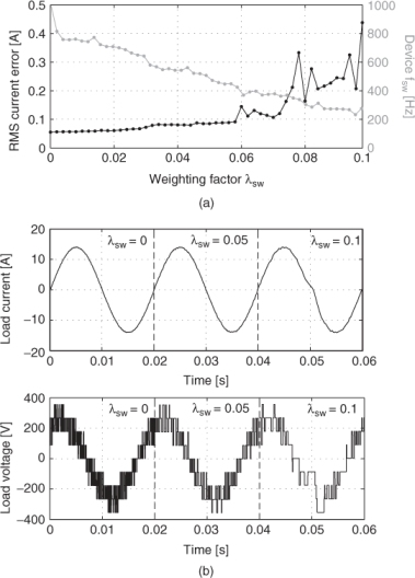
It can be observed in these results that a reduction in the switching frequency introduces higher distortion, affecting the quality of the load current. This trade-off is very clear in Figure 11.2a since the curves representing each measure have opposite evolutions for the different values of λ_sw. A suitable selection of λ_sw would be any value in since the current error is still below 10% of the rated current (15 A in this example) and a reduction from 1000 to 500 Hz is achieved for the average device switching frequency. Finally λ_sw = 0.05 has been selected. In this application it is also possible to select λ_sw in order to achieve a given switching frequency.

Figure 11.2b shows comparative results for the system working with three different values of λ_sw, one of them the selected value. Note how the load current presents higher distortion for the larger value of λ_sw due to the strong reduction in the number of commutations. On the other hand, for λ_sw = 0 the current control works at its best, but at the expense of higher switching losses. Since the NPC is intended for medium-voltage, high-power applications where losses become important, the selection of λ_sw = 0.05 merges efficiency with performance. A comparison of this predictive method and a traditional PWM-based controller can be found in [8].

11.4.2 Common-Mode Voltage Reduction

The guidelines presented in this chapter have been used to tune the weighting factor of the second equation in Table 11.2. This example corresponds to the predictive current control of a matrix converter with reduction of the common-mode voltage [9], using the following cost function:

11.3

where the additional term is the predicted common-mode voltage for the different switching states and will be considered a secondary objective of the control; its effect is adjusted by properly tuning the weighting factor λ_cm.

The predictive current control strategy for the matrix converter is explained in Chapter 7. The common-mode voltage is defined as

11.4

where the output voltages v_aN, v_bN, and v_cN are calculated as a function of the voltages at the input of the matrix converter and the converter switching states. Common-mode voltages cause overvoltage stress in the winding insulation of the electrical machine fed by the power converter, producing deterioration and reducing the lifetime of the machine. In addition, capacitive currents through the machine bearings can damage them, and electromagnetic interference can affect the operation of electronic equipment. By including this secondary term in the cost function the common-mode voltage and its negative effects can be reduced.

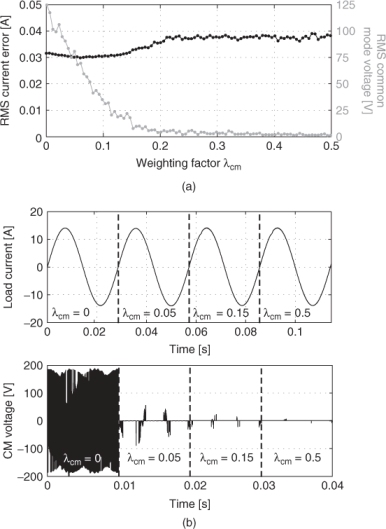
The measures that will be used to evaluate the performance of the different values of λ_cm are the RMS current error and the RMS common-mode voltage. Results showing both measures obtained from a series of simulations for several values of λ_cm are presented in Figure 11.3a. Note that, as in the previous example, similar evolutions of both measures are obtained, that is, for higher values of λ_cm smaller common-mode voltages are obtained, while the current control becomes less important and loses some performance. The results also show that the common-mode voltage is a variable that is more decoupled from the load current, compared to the switching frequency, since the current error remains very low throughout a wide range of λ_cm. Hence the selection of an appropriate value is easier, and values of will perform well. This can be seen for the results shown in Figure 11.3b, where clearly a noticeable reduction in the common-mode voltage is achieved without affecting the current control.

Figure 11.3 (a) Weighting factor influence on the current error and the common-mode voltage. (b) Results comparison for different weighting factors (load current and common-mode voltage) (Cortes et al., 2009 © IEEE)

11.4.3 Input Reactive Power Reduction

Predictive current control with a reduction of the input reactive power in a matrix converter was proposed in [10, 11]. This control scheme and the required system models are explained in Chapter 7. The cost function for this control scheme consists of a primary term for output current control, expressed in orthogonal coordinates, and a secondary term for reduction of the input reactive power:

11.5

The additional term in the cost function is the predicted input reactive power Q^p with its corresponding weighting factor λ_Q.

In order to evaluate and select the value of λ_Q, the measures of performance of the system are the RMS current error and the input reactive power magnitude Q.

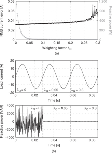
The results of the tuning procedure are depicted in Figure 11.4a. Since this cost function belongs to the same classification as the previous two examples, it is expected to present similar measurement evolution with increasing λ_Q. As in the previous case, the input reactive power seems to be very decoupled from the load current, hence the current error remains very low for a wide range of λ_Q. It becomes easy to obtain a suitable value by considering . This can be corroborated by the results given in Figure 11.4b, showing an important reduction of the input reactive power for λ_Q = 0.05.

Figure 11.4 (a) Weighting factor influence on the current error and the input reactive power. (b) Results comparison for different weighting factors (load current and input reactive power) (Cortes et al., 2009 © IEEE)

11.4.4 Torque and Flux Control

A good example of a cost function with equally important terms is the predictive torque and flux control for an induction machine, which is explained in Chapter 8. Here, the objective of the control algorithm is to simultaneously control the electrical torque T_e and the magnitude of the stator flux . This objective can be expressed as a cost function with two terms, torque error and flux error, and the weighting factor must handle the difference in magnitude and units between these two terms, as proposed in [12]. A different approach consists of using a normalized cost function where each term is divided by its rated value, resulting in

11.6

Using this cost function, the same importance is given to both terms using λ_ψ = 1, as proposed in [13]. However, the optimal value can be different, depending on the defined criteria for optimal operation.

In order to evaluate the performance of the control for different values of the weighting factor λ_ψ, the RMS torque error and RMS stator flux magnitude error are defined as measures of performance.

A branch and bound algorithm starting with λ_ψ = 0.01,0.1,1,10, and 100 first gave the interval , and then , with very small differences. Finally λ_ψ = 0.85 was chosen. Note that the obtained optimal value is very close to the initial value of λ_ψ = 1.

Figure 11.5a shows extensive results considering many more values of λ_ψ (note that the values are represented in log₁₀ scale), to show that the branch and bound method really has found a suitable solution.

Figure 11.5 (a) Weighting factor influence on the flux and torque errors. (b) Results comparison for different weighting factors (torque step response, flux magnitude at steady state, and load currents) (Cortes et al., 2009 © IEEE)

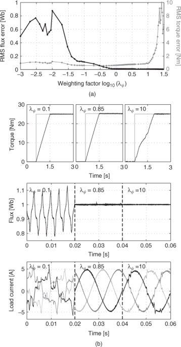
Results for different values of λ_ψ, including λ_ψ = 0.85, are given in Figure 11.5b to show the performance achieved by the predictive torque and flux control. Note that λ_ψ = 0.85 presents a very good combination of torque step response and steady state, flux control, and load current waveforms.

11.4.5 Capacitor Voltage Balancing

As presented in Chapter 5, the NPC inverter has two DC link capacitors in order to generate three voltage levels at the output of each phase. These voltages need to be balanced for proper operation of the inverter. If this balance is not controlled, the DC link voltages will drift and introduce considerable output voltage distortion, not to mention that the DC link capacitors could be damaged by overvoltage, unless they are overrated.

This control requirement can be considered in the predictive current control scheme by introducing an additional term in the cost function. The resulting cost function is expressed as

11.7

where is the predicted voltage unbalance and λ_ΔC is the weighting factor to be adjusted. Note that the cost function terms have been normalized considering the values of rated current i_sn and rated DC link capacitor voltage V_cn, as indicated in the first step of the adjustment procedure.

The measures that will be used to evaluate the weighting factor λ_ΔC are the RMS values of the current error and of the voltage unbalance.

A branch and bound algorithm starting with λ_ΔC = 10⁻², 10⁻¹, 1, 10¹, and 10² first gave the interval ; after this first evaluation two additional iterations were necessary until very small differences were obtained between the extremes of the interval. Finally λ_ΔC = 1.05 was chosen. Figure 11.6a shows extensive results considering many more values (note that the values are represented in log₁₀ scale), to show that the branch and bound method really has found a suitable solution.

Figure 11.6 (a) Weighting factor influence on the current error and the DC link capacitor unbalance. (b) Results comparison for different weighting factors (load current and DC link capacitor voltages, dynamic behavior) (Cortes et al., 2009 © IEEE)

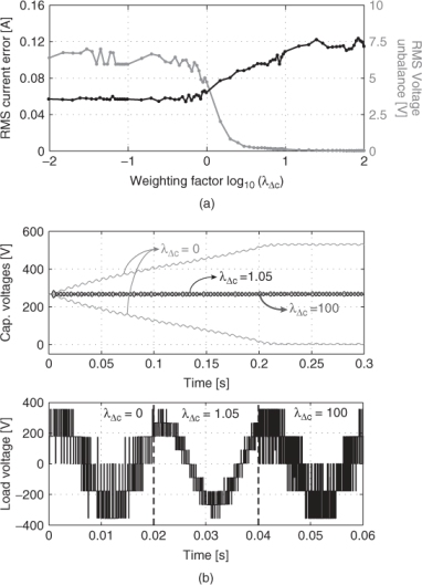
Results for different λ_ΔC, including λ_ΔC = 1.05, are given in Figure 11.6b to show the performance achieved by the MPC. Note that for λ_ΔC = 0, which normally is not allowed since it does not control the unbalance producing the maximum drift of the DC link capacitors, the load voltage only presents five different voltage levels, while nine levels should appear in the load phase-to-neutral voltage (since the NPC has three levels in the converter phase-to-neutral voltage). Only five appear since the NPC is not generating three output levels but only two, due to the voltage drift of its capacitors. On the other hand, λ_ΔC = 100 controls the voltage unbalance very accurately; it even makes voltage unbalance so important in the cost function that it avoids generation of those switching states that produce unbalance, eliminating voltage levels at the output and increases the switching frequency, as can be seen in the load voltage of Figure 11.6b. Finally, the selected weighting factor value λ_ΔC = 1.05 presents the nine load voltage levels, controls the load current, and keeps the capacitor voltages balanced.