4.8 Implementation of the Predictive Control Strategy

A flow diagram of the different tasks performed by the predictive controller is shown in Figure 4.8. Here, the outer loop is executed every sampling time, and the inner loop is executed for each possible state, obtaining the optimal switching state to be applied during the next sampling period.

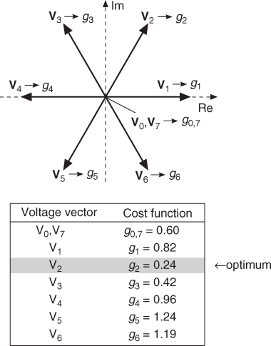
Figure 4.7 Working principle: values of the cost function for each voltage vector

The timing of the different tasks is shown in Figure 4.9, and, as illustrated here, the most time-consuming task is the prediction and selection of the optimal switching state. This is due to the calculation of the load model and cost function, which is executed seven times, once for each different voltage vector.

Figure 4.8 Flow diagram of the predictive current control (Rodriguez et al., 2007 © IEEE)

The predictive current control strategy is implemented for simulation in MATLAB as a S-Function, containing the following code:

    ek = v(xop_1) - L/Ts*ik - (R-L/Ts)*ik_1;
    g_opt = inf;
    for i=1:7
        ik1 = (1-R*Ts/L)*ik + Ts/L*(v(i)-ek);
        g = abs(real(ik_ref-ik1)) + abs(imag(ik_ref-ik1));
        if (g<g_opt)
            g_opt = g;
            x_opt = i;
        end
    end
    xop_1=xop;
    xop=x_opt;

where ik = i(k), ik1 = i(k + 1), ik_1 = i(k − 1), and ek = e(k). The optimal voltage vector that minimize the error is v(xop).

When the predictive control is implemented experimentally, the same code is rewritten in C language with alpha and beta currents calculated separately.

Results using the control algorithm implemented in MATLAB/Simulink are shown next, considering (4.22) for load current prediction and (4.23) for back-emf estimation. The system parameters V_dc = 520 V, L = 10 mH, R = 10 Ω, and e = 100 V_peak have been considered for simulations.

Current and voltage in one phase of the load are shown in Figure 4.10 for a sampling time T_s = 100 μs. There is no steady state error in the current but there is a noticeable ripple. This ripple is reduced considerably when a smaller sampling time is used, as shown in Figure 4.11 for a sampling time T_s = 25 μs. However, by reducing the sampling time, the switching frequency is increased as can be seen by comparing the load voltages in Figure 4.10 and Figure 4.11.

Figure 4.9 Timing of the different tasks (Rodriguez et al., 2007 © IEEE)

Figure 4.10 Steady state load current and voltage for a sampling time T_s = 100 μs

Real and estimated back-emf are shown in Figure 4.12. Back-emf is estimated using (4.23) with a sampling time T_s = 25 μs.

Figure 4.11 Steady state load current and voltage for a sampling time T_s = 25 μs

The response of the system to a step in the amplitude of the reference current vector i^* is shown in Figure 4.13. It can be observed that the load currents follow their references with fast dynamics. It is also shown in this figure how the load voltage changes during the reference current step.

Figure 4.12 Real and estimated back-emf

The predictive current control strategy was implemented with the experimental setup described in Figure 4.14. A Danfoss VLT5008 5.5 kW three-phase inverter with an RL load is used. The DC link is fed by a three-phase diode bridge rectifier. The inverter is controlled externally through an interface and protection card (IPC). A TMS320C6713 floating-point DSP was used for the control. The gate drive signals for each inverter leg are sent from the DSP to the IPC through fiber optic cables. Current measurements of two phases are sent back from the inverter to the DSP through coaxial cables. A FPGA-based daughter card handles the analog to digital conversion, digital to analog conversion, and the digital outputs for the DSP. The execution time for the implemented current control algorithm was about 7 μs. The parameters of the experimental setup are V_dc = 520 V, L = 10 mH, R = 10 Ω, e = 0 V_peak, and T_s = 25 μs.

Figure 4.13 Load currents for a step in the amplitude of the reference current vector i^*, with sampling time T_s = 25 μs

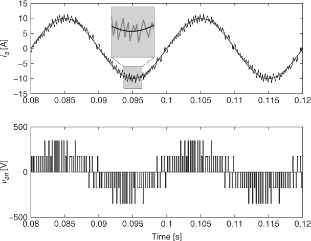
The behavior of the load currents and the voltage in one phase at steady state operation is shown in Figure 4.15. The amplitude of the reference current was set to 10 A with a frequency of 50 Hz. Currents are sinusoidal with low harmonic distortion.

Figure 4.14 Overview of experimental system setup

Results for a step change in the amplitude of the reference from 5 to 10 A are shown in Figure 4.16. The amplitude of the reference current is kept at 10 A. It can be observed that the load current i_α reaches its reference with very fast dynamics while i_β is not affected by this step change. This result shows that the currents are decoupled in the predictive current control scheme. The load voltage v_an for the same test is shown in Figure 4.17. It can be seen that during the step change of current i_α the load voltage is kept at its maximum value until the reference current is achieved.

Figure 4.15 Experimental results in steady state. Load currents and voltage in one phase of the load

Figure 4.16 Experimental results for a step in the amplitude of . Load currents

The behavior of the load currents and load voltage for a step in the amplitude of the reference current vector is shown in Figure 4.18. The amplitude of the reference current changes from 10 to 5 A and later from 5 to 10 A for all phases. The reference current is also shown in the figure. It can be seen that the amplitude of the load currents changes very quickly following the change of the reference. It is also shown in the figure how the load voltage v_an changes during this test.

Figure 4.17 Experimental results for a step in the amplitude of . Load current and voltage