
7.4 Predictive Current Control of the Matrix Converter
7.4.1 Model of the Matrix Converter for Predictive Control
7.4.1.1 Matrix Converter Model
For predictive control the model of the MC is extremely simple: it considers only (7.2) and (7.5), which relate the instantaneous values of input and output currents and voltages. Based on the restriction presented by (7.1), the MC has 27 different switching states to be considered for prediction of the variables.
7.4.1.2 Load Model
In this case the objective is to obtain an equation to predict the value of the load current in the next sampling interval, for each of the 27 different switching states of the MC. The equation for the resistive–inductive–active load presented in Figure 7.1 is
where L and R are the inductance and resistance of the load and e is the electromotive force (emf). This load model is quite general, because it covers a wide variety of applications such as passive inductive load, motors, and grid-connected converters.
Considering the approximation for the derivative of the output current
where Ts is the sampling period, the equation for predicting the load current is obtained from substituting (7.22) into(7.23), which gives
where io(k + 1) is the predicted value of the current for sampling interval k + 1, for different values of vo(k). The corresponding load voltage vector vo(k) is calculated for all the 27 switching states of the converter.
The present value of load back-emf e(t) can be estimated using a second-order extrapolation from present and past values, or considering e(k − 1) ≈ e(k), depending on the sampling time. For sufficiently small sampling time, no extrapolation is needed.
7.4.1.3 Input Filter Model
The input filter model, based on the circuit shown in Figure 7.1, can be described by the following continuous-time equations:
where Lf and Rf are the joint inductance and resistance of the line and filter and Cf is the filter's capacitance and:
![]()
This continuous-time system can be rewritten as
with
7.28 ![]()
A discrete state space model can be derived when a zero-order hold input is applied to a continuous-time system described in state space form as in (7.27). Considering a sampling period Ts, the discrete-time system derived from (7.27) is
with
7.30 ![]()
For more details on sampled-data systems and the theory employed in this analysis, see [5]. The discrete-time variables will match the continuous-time variables at sampling intervals. A convenient way of obtaining the discrete model is through MATLAB® function c2d():conversionofcontinuous − timemodelstodiscretetime. To predict the mains current, it is necessary simply to solve is(k + 1) from (7.29):
At this point, the method can use this model to predict the value of is depending on ii. Then (7.5) must be used to calculate ii for each switching state.
7.4.1.4 The Instantaneous Reactive Power
The behavior of the MC can be improved by considering the instantaneous reactive power Q in the three-phase grid.
This reactive power is calculated by the following equation [6]:
7.32 ![]()
where Im{} corresponds to the imaginary part of the product of the vectors and ![]() is the complex conjugate of is(t).
is the complex conjugate of is(t).
The instantaneous reactive power can be predicted by using
where the subscripts α and β represent the real and imaginary components of the associated vector. The predicted value for the input current is(k + 1) is obtained from (7.31). Line voltages are low-frequency signals and it can be considered that vs(k + 1) ≈ vs(k).
7.4.2 Output Current Control
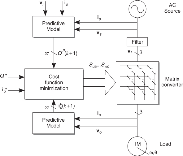
A block diagram of the predictive current control scheme for the MC is shown in Figure 7.5 considering an induction machine (IM) as the load. The load model and the filter model are used for calculating predictions of the future values of the output current for the 27 switching states of the MC. Based on these predictions, a cost function is used for selection of the optimal switching state to be applied in the converter.
Figure 7.5 Block diagram of the predictive current control strategy
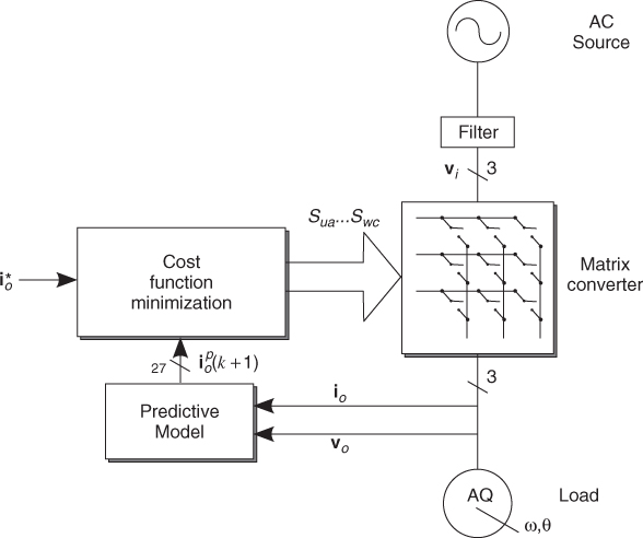
The cost function g represents the evaluation criterion by which the control method determines the optimum switching state to be applied during the next sampling time. The optimization process is performed by evaluating g for each valid switching state. But prior to determining the equation that will represent the cost function, it is necessary to define the objectives that the converter must achieve. The MC must feed the load with currents close to the reference value and, at the same time, allow control of the input current in order to get low harmonic distortion and regulated power factor (PF). Several other objectives can be included in the cost function due to the versatility of the presented approach, opening up a wide range of possibilities for further research.
One of the objectives reflected in the cost function is the tracking of the reference current to the load. Switching states that generate closer values of the output current to the reference should be preferred. That goal is achieved by assigning cost or penalizing differences from the reference value, as expressed in the following cost function:
7.34 ![]()
where currents ![]() and
and ![]() are the real and imaginary parts of the reference current vector i*. Currents
are the real and imaginary parts of the reference current vector i*. Currents ![]() and
and ![]() are the real and imaginary parts of the predicted current vector ip(k + 1) calculated using (7.24) for a given switching state.
are the real and imaginary parts of the predicted current vector ip(k + 1) calculated using (7.24) for a given switching state.
The behavior of the predictive control scheme for the MC is shown next for an 11 kW induction machine fed by an 18 kVA MC.
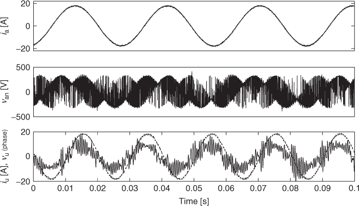
The predictive control scheme implemented without control of reactive power presents good reference tracking for the output currents, as shown in Figure 7.6. However, the input currents are very distorted and the input power factor is not controlled.
Figure 7.6 Steady state operation of the load current control without control of the input reactive power (Vargas et al., 2008 © IEEE)
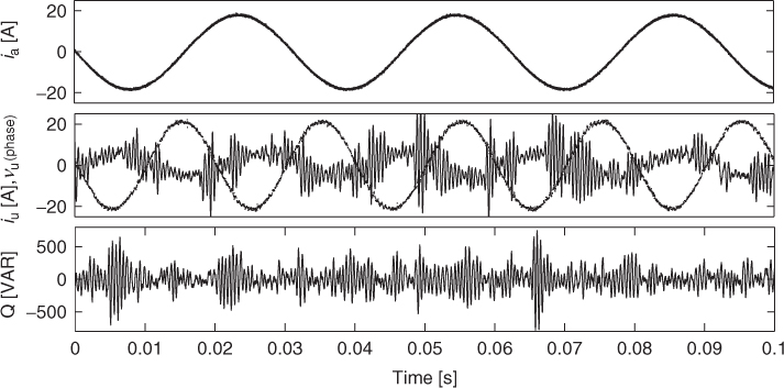
One of the advantages of the MC topology is the capacity for regeneration, that is, power flowing from the load to the grid. The operation of the MC in regeneration conditions is shown in Figure 7.7 for current control without regulation of the input power factor. It can be observed that the output current control maintains its good performance while the input currents are distorted.
Figure 7.7 Steady state in regeneration without control of the input reactive power (Vargas et al., 2008 © IEEE)
7.4.3 Output Current Control with Minimization of the Input Reactive Power
The MC can control, in addition to the output currents, the phase of the input current from the mains. The amplitude is determined by the active power flow, since the MC does not store energy. Most modulation methods reach the objective of working with unity power factor by means of relatively complex strategies [7, 8]. In order to work with inductive or capacitive power factor, the complexity increases considerably [9–11]. With the predictive control approach, the objective of controlling the reactive power Q can be easily achieved simply by penalizing switching states that produce predictions of Q distant from the reference value [12, 13]. That is
7.35 ![]()
The value of the predicted reactive power Qp is obtained for each valid switching state from (7.33). Its reference value Q* is given externally, as shown in Figure 7.5, to work with capacitive, inductive, or unity power factor (PF). Most applications require unity PF, hence Q* = 0 and g2 = |Qp|, but this method offers the alternative to control that variable with a very simple approach compared to other modulation strategies [9–11].
The resulting cost function that reflects both objectives, output current and reactive input power control, is obtained simply by adding g1 and g2, thus
where the weighing factor A handles the relevance of each objective. In order to deal with the different units of the terms present in g, A must have V−1 as unit.
A block diagram for the predictive control of the MC considering the input reactive power minimization is shown in Figure 7.8. Compared to the control scheme from Figure 7.5, the model of the input filter has been added and the cost function is the one presented in (7.36).
Figure 7.8 Block diagram of the predictive current control strategy with minimization of the input reactive power
A higher value of A implies a higher relevance for controlling the PF or reactive input power over the output current reference tracking. The criteria for selecting the value of A are briefly treated next.
7.4.3.1 Selection of Weighting Factor A
Weighting factor A is the only parameter from the predictive current controller to be adjusted. The adjustment of this kind of parameter is still an open topic for research. It is possible to find optimal values in cases where the system presents no constraints and under specific structures of the cost function [14]. For systems with a finite number of control actions, finite input sets, or state alphabet [15], one method to adjust the parameter is to simply evaluate the performance of specific system variables by simulations to determine the best value.
For the presented MC-based system, key variables for evaluating the behavior of the predictive current control method are the total harmonic distortion (THD) of the output and input or mains current. In order to perform the evaluation, an exhaustive search was carried out based on 400 simulations, each with an equidistant value of A within the range 0–0.007 V−1. As mentioned, the variables to observe and evaluate in order to select the weighing factor are the input and output current THD. The result of this procedure is shown in Figure 7.9.
Figure 7.9 Exhaustive search to evaluate and select parameter A (Vargas et al., 2008 © IEEE)
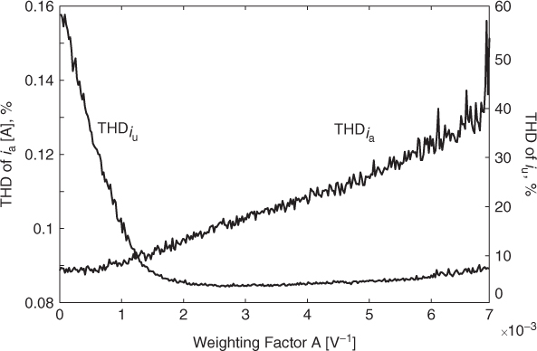
As expected, the input current's THD drastically decreases as A increases, reaching a value close to 5%
near A = 0.002 V−1. No further reduction is significant after that value of A. On the other hand, as a trade-off, the output current's THD increases as more importance is placed on the reactive power in the cost function as A increases. Although the output current's THD is still low within the evaluated range–values from 0.09%
to 0.14%
are not considered to be high distortion–the ideal situation is to achieve low distortion on both currents. For that reason, the weighing factor A was set at A = 0.0045 V−1, to select a value far from the region where the input current's THD drastically increases (under A = 0.002 V−1) and not higher, in order to ensure low THD on the output current, according to the results shown in Figure 7.9.
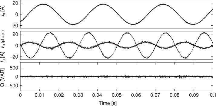
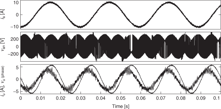
In order to obtain unity PF a reactive power reference Q* = 0 is set. Results for these conditions are shown in Figure 7.10. It can be observed that the good quality of the output current control is maintained, compared to the results of Figure 7.6, while the waveform of the input currents is greatly improved. The input currents are sinusoidal with low distortion and in phase with the grid voltages. Control of the input PF is achieved even during regenerative operation of the converter, as shown in Figure 7.11.
Figure 7.10 Steady state operation of the load current control with minimization of the input reactive power (A = 0.0045) (Vargas et al., 2008 © IEEE)
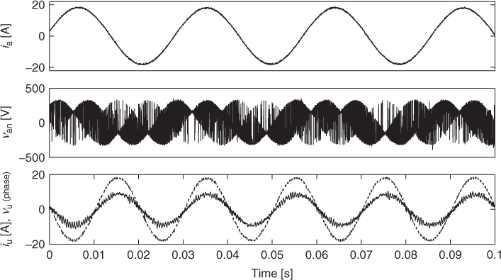
Figure 7.11 Steady state in regeneration using the load current control with minimization of the input reactive power (A = 0.0045) (Vargas et al., 2008 © IEEE)
7.4.4 Input Reactive Power Control
The capability of this control method to regulate the input PF is shown in Figure 7.12 for a reactive power reference of Q* = 900 VAR. The parameter A is set to 0.0045.
Figure 7.12 Performance of the drive with capacitive PF (Q* = 900 VAR), A = 0.0045 (Vargas et al., 2008 © IEEE)
Results for Q* = 0 VAR (unity PF) can be seen in Figure 7.10. No difference is observed in terms of the output behavior of the converter. The main difference, as expected, is in the behavior of the input current, presenting a capacitive PF of 0.81. Consequently, it is possible to control the input PF by changing the value of Q*.