10.3 Actuation Constraints
In a control system it is important to reach a compromise between reference following and control effort. In power converters and drives, the control effort is related to the voltage or current variations, the switching frequency, or the switching losses. Using predictive control, it is possible to consider any measure of control effort in the cost function, in order to reduce it.
In a three-phase inverter, the control effort can be represented by the change in the voltage vector applied to the load. This can be implemented as an additional term in the cost function measuring the magnitude of the difference between the previously applied voltage vector v(k − 1) and the voltage vector to be applied v(k), resulting in
where x is the controlled variable and λ is a weighting factor that allows the level of compromise to be adjusted between reference following and control effort.
As an example, the predictive current control presented in Chapter 4 is considered, together with the constraint in the variation of the voltage vectors presented in (10.8). The resulting cost function is expressed as
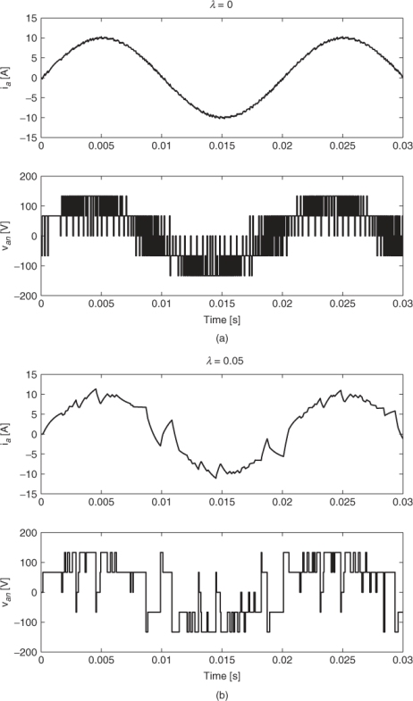
By using this cost function, the control effort can be reduced by increasing the value of the weighting factor λ. Results for the current control of a three-phase inverter using cost function (10.9) are shown in Figure 10.1. It can be seen that by reducing the voltage variation, the load voltage is maintained for several sampling periods at a fixed value, reducing the switching frequency fsw from 2767 to 723 Hz, with a negative effect on the current reference following. For both results the sampling frequency is the same, fs = 20 kHz.
Figure 10.1 Predictive current control with reduction of the voltage variation using cost function (10.9). (a) Switching frequency fsw = 2767 Hz. (b) Switching frequency fsw = 723 Hz
Results for low switching frequency can be improved by considering a squared error for the current reference following terms of the cost function
Results for this cost function are shown in Figure 10.2. It can be observed here that for a switching frequency that is similar to the one obtained in Figure 10.1b, the current and voltage waveforms present a considerably better performance, with lower current and voltage distortion.
Figure 10.2 Predictive current control with reduction of the voltage variation using cost function (10.10). Switching frequency fsw = 725 Hz

10.3.1 Minimization of the Switching Frequency
As in power converters, one of the major measures of control effort is the switching frequency. It is important in many applications to be able to control or limit the number of commutations of the power switches.
To directly consider the reduction in the number of commutations in the cost function, a simple approach is to include a term in it that covers the number of switches that change when the switching state S(k) is applied, with respect to the previously applied switching state S(k − 1).
The resulting cost function is expressed as
where n is the number of switches that change when the switching state S(k) is applied.
If the switching state vector S is defined as
10.12 ![]()
where each element Sx represents the state of a switch and has only two states, one or zero, then the number of switches that change from S(k − 1) to S(k) is
10.13 
Considering the three-phase inverter as an example, the switching state vector S = (Sa, Sb, Sc) defines the switching state of each inverter leg. Then the number of switches changing from time k − 1 to time k is
10.14 ![]()
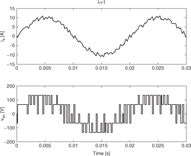
The behavior of the switching frequency for different values of the weighting factor λn is shown in Figure 10.3. It can be seen that the switching frequency can be reduced to the required value by increasing the weighting factor. Results for the three-phase inverter operating at fsw = 525 Hz are shown in Figure 10.4.
Figure 10.3 Predictive current control with reduction of the switching frequency using cost function (10.11)
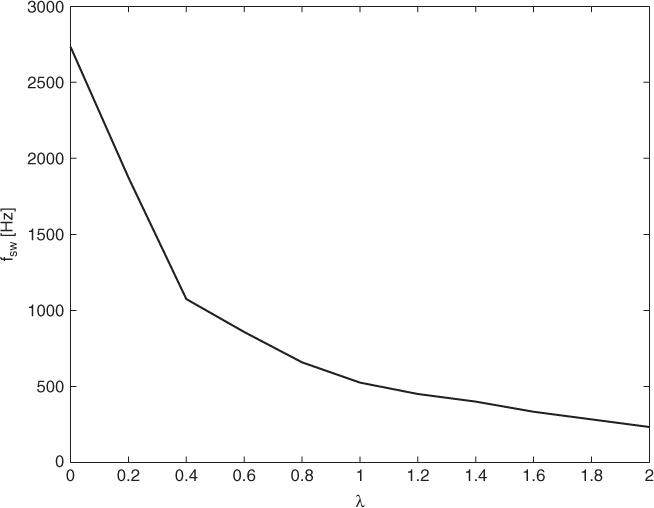
Figure 10.4 Predictive current control with reduction of the switching frequency using cost function (10.11). Switching frequency fsw = 525 Hz
A similar strategy, applied to a three-level neutral-point clamped (NPC) inverter, was presented in [4].
10.3.2 Minimization of the Switching Losses
Considering that the switching losses depend not only on the switching frequency but also on the voltage and current values at the moment of switching, a simple model of the switching process can be considered for direct minimization of the switching losses using predictive control.
The energy loss of one switching event can be calculated based on the values of the switched voltage Δvce and current Δic. The use of a polynomial considering all the physically reasonable terms is proposed in [5]:
where the coefficients K1, … , K5 are obtained from a least squares approximation of the measured data.
In order to obtain a simplified expression for estimating the losses, it is possible to neglect several of the terms in (10.15) by considering the experimental data, resulting in
10.16 ![]()
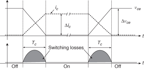
This expression is equivalent to the resulting equation obtained from considering the simplified current and voltage waveforms during the commutation process shown in Figure 10.5. From this figure it is possible to calculate the dissipated energy during the commutation process by integrating the instantaneous power:
10.17 ![]()
or
10.18 ![]()
where Tc is the duration of the commutation.
Figure 10.5 Simple model for estimation of the switching losses
This simple model for estimating the switching losses can be included in the cost function as a term that also includes the predicted losses of all the switches of the power converter:
10.19 
where N is the number of switching devices in the converter.
This control strategy for reducting the switching losses was proposed for a matrix converter in [6]. This work considers a cost function for output current control, input reactive power minimization, and reduction of switching losses:
10.20 
where io = ioα + ioβ is the output current vector, Q is the input reactive power, and A and B are weighting factors. A detailed explanation of the predictive control of the matrix converter is presented in Chapter 7.
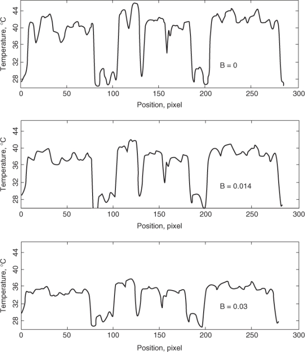
It was shown in [6] that by adjusting the value of B the efficiency of the matrix converter can be increased, maintaining the good performance, in terms of THD, of the input and output currents. By using a higher value of B the switching losses can be further reduced, but the THD of the currents will be increased. The temperature of the matrix converter switches, obtained using a thermal camera, is shown in Figure 10.6 for different values of B. It can be seen in the figure that as the value of B increases, the temperature of the switches decreases, as a result of lower switching losses.
Figure 10.6 Temperature of the IGBTs for different values of B (Vargas et al., 2008 © IEEE)