CPU Usage

When applications are running slow, the first thing you should check is whether the system is in fact busy doing anything. The quickest way to find out is via the uptime command , as shown in Listing 17-1.

Listing 17-1. The uptime Command

$ uptime
12:51:04 up 116 days, 7:09, 3 users, load average: 0.01, 0.07, 0.02

This command prints a short overview of the system status, including the current time, the amount of time the system has been on (or up), the number of logged-in users, and three numbers representing the system’s workload.

In our example, the system was last booted 116 days, 7 hours, and 9 minutes ago. If you lose connectivity with a remote server, this allows you to easily determine whether the system was rebooted once you can log back in.

The number of logged-in users is the total number of current logins via the terminal console, in X, and via SSH. If you are logged in twice, you will be counted as two users. Users connected to a service like Samba or Apache are not counted here.

Finally, the system load is displayed in three numbers. These numbers form an index that indicates the average ratio of work scheduled to be done by a CPU versus the work actually being done, over the past 1-minute, 5-minute, and 15-minute periods.

A load of 1.00 means the amount of work being scheduled is identical to the amount of work a CPU can handle. Confusingly, if a host contains multiple CPUs, the load for each CPU is added to create a total; on a host with four CPU cores, a load of 4.00 means the same as a load of 1.00 on a single-core system.

In our example, the average workload over the past minute was about 1 percent. Some extra tasks were running and probably completed a few minutes ago, as the average workload over the past 5 minutes was 7 percent.

Though these numbers should by no means be taken as gospel, they do provide a quick way to check whether a system is likely to be healthy. If the system load is 6.00 on a host with eight CPU cores, a lot of tasks may have just finished running. If the load is 60, a problem exists.

This problem can be that the host is running a few processes that monopolize the CPU, not allowing other processes enough cycles. We’ll show you how to find these processes with the top utility a bit later. Alternatively, your host might be trying to run far more processes than it can cope with, again not leaving enough CPU cycles for any of them. This may happen if a badly written application or daemon keeps spawning copies of itself. See the “Fork Bomb” sidebar for more information. We’ll show you how to prevent this using the ulimit command later.

Finally, it’s possible that a process is waiting for the host to perform a task that cannot be interrupted, such as moving data to or from disk. If this task must be completed before the process can continue, the process is said to be in uninterruptible sleep. It will count toward a higher load average but won’t actually be using the CPU. We’ll show you how to check how much the disk is being used in the “Advanced Tools” section a bit later.

Memory Usage

Another cause of reduced performance is excessive memory use. If a task starts using a lot of memory, the host will be forced to free up memory for it by putting other tasks into swap memory. Accessing swap memory , which after all is just a piece of disk that is used as if it were memory, is very slow compared to accessing RAM.

You can quickly check how much RAM and swap memory a host is using via the free command. We’ll pass it the -h (human-readable) option so it displays the sizes in gigabytes (-g), megabytes (-m), or kilobytes (-k), as in Listing 17-2.

Listing 17-2. The free Command

$ free -h
               total        used        free      shared       buff/cache     available
Mem:           3.1G         59M         2.7G      13M          350M           2.8G
Swap:          1.5G         0B          1.5G

This listing gives you an instant overview of whether the system is running low on available memory. The first line tells you the status of RAM use. The total is the amount of RAM that is available to this host. This is then divided into RAM that is in use and RAM that is free. Different versions of the free program may show different memory values on the same system.

The shared refers to shared memory, mainly tmpfs. This matches the /proc/meminfo Shmem value (space used by the kernel).

The buffers column tells you the amount of memory the kernel is using to act as a disk write buffer. This buffer allows applications to write data quickly and have the kernel deal with writing it to disk in the background. Data can also be read from this buffer, providing an additional speed increase. The last column, cached, tells you how much memory the kernel is using as a cache to have access to information quickly.

Both the buffer and cache are resized as needed. If an application needs more RAM, the kernel will free up part of the cache or buffer space and reallocate the memory. If swap space is available, the kernel can move inactive memory to the swap space.

Finally, the last line tells us how much swap space the host is using. Over time, this number will rise slightly, as services that aren’t being used can be parked in swap space by the kernel. Doing this allows it to reclaim the otherwise idle RAM and use it as buffer or cache.

This means that having your host use swap space is not necessarily a bad thing. However, if all memory and all swap space are in use, there is obviously a problem. In our case, we are not using any swap space and so it is showing as 0s out of a possible 1.5GB available to us.

We’ll show you how to find out how much memory individual tasks are using in the “Advanced Tools” section.

Disk Space

The other finite resources a computer system has are disk space and disk speed. Generally speaking, a system won’t slow down when a disk becomes full, but services may crash and cause your users grief, so it pays to keep an eye on usage and make more storage available when needed.

We’ll show you how to check for disk speed problems in the next section.

Logs

Finally, if something untoward has occurred with an application or the kernel, you’ll likely find a log entry in your system or kernel log. You will of course want to restart any service that crashed, but checking the logs for the cause of the problem will help you prevent the same thing from happening again.

If the log daemon itself has stopped, you can still check the kernel log buffer via the dmesg command.

CPU and Memory Use

To list details about currently running tasks, Linux provides the top utility. This is similar to the Task Manager you may be used to from Windows or Activity Monitor on macOS, but it runs in a terminal window, as shown in Figure 17-1. It provides a sortable and configurable listing of running processes and threads on the host. You access it with the following command:

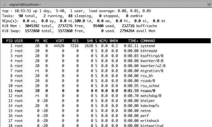
Figure 17-1. The top utility

$ top

The top of the output gives you a few header lines, which includes the information from uptime, as well as some aggregated data from the free and vmstat commands, which we’ll discuss in the “Swap Space Use” and “Disk Access” sections a bit later. You can toggle these headers on and off. The L key toggles the display of the load average line. You can toggle the task summary via the T key and memory information via M.

The rest of the display consists of several columns of information about running processes and threads. The columns you see here are shown by default, but you can enable or disable others as well. We’ve listed their headers and meaning in Table 17-1.

You can obtain full descriptions for these and all other available fields in the man top manual page.

By default, the tasks are displayed in descending order and sorted by %CPU. The process consuming the most CPU time will be at the top of the list, which is immediately useful for problem solving.

We can sort on many columns in top. To sort on CPU usage, we will need to sort the %CPU column. We can choose a column to sort by pressing the F key, which brings up a list of available columns, as shown in Figure 17-2.

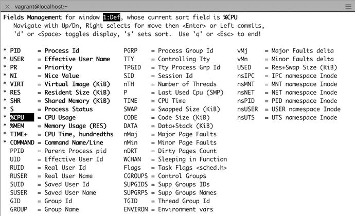
Figure 17-2. Choosing a sort field

The first line tells us the current sort field, %CPU. Below that we have instructions on how to choose a different sort field. The up and down arrows navigate to the different fields. If you press s, you will see that that field is now selected. The d key and spacebar toggle whether that field will be displayed. You can use q or the Escape key to go back to the top screen with your selection. We can press s to make the %CPU column our sort field and then press q to go back to the task list. All processes are now sorted by the number of CPU cycles they use, so if a process is running amok, you’ll be able to spot it easily.

$ ps aux |grep Z
USER    PID    %CPU %MEM   VSZ   RSS   TTY     STAT    START   TIME   COMMAND
ubuntu  7814   0.0  0.0    0     0     pts/0   Z+      11:52   0:00   [zombie] <defunct>

Many more display options are available in top, and you can find them on the help menu. Press ? to access it. When you have customized the way top displays information to your liking, you can save the configuration by pressing W. This will write the settings to a file called .toprc in your home directory.

If you find a misbehaving task, you can use top to quit it. To do this, press k and enter the PID of the task in question. You will then be asked for the signal to send to the process. The signal to make a process terminate normally is 15. If this doesn’t work, you might want to try sending signal 3, which is a bit sterner, or signal 9, which is akin to axe-murdering the process.

To find out more about signals, read the “Killing Is Not Always Murder” sidebar.

If you have a process that is using too much CPU time and interrupting more important processes, you can try making it nicer, by lowering its priority. This means it will yield more easily to other processes, allowing them to use some of the CPU cycles that were assigned to it. You can change process niceness by pressing the R key. top will ask you for the process ID and then the new niceness value.

Unless you run top as root or via sudo, you can only make processes nicer. You cannot raise their priority, only lower it.

When done, press q to quit top.

Swap Space Use

If you see a lot of swap space in use, it may indicate the system is running low on memory. Swap space and RAM make up the total allocatable memory available to your system. The kernel will swap out less used memory pages into the swap space when it requires memory for a particular process and does not have that immediately available. This isn’t necessarily a bad thing, but if the system is “heavily swapping” (that is, moving memory pages in and out of swap space frequently, then because swap is much slower than RAM, it can lead to poor performance).

You can check whether this is the case via the vmstat utility. You normally want to tell this utility to print information every few seconds so you can spot any trends. Pass the -n option to prevent the headers from being reprinted and tell it to redisplay statistics every 5 seconds, as shown in Figure 17-3. Press Ctrl+C to quit vmstat.

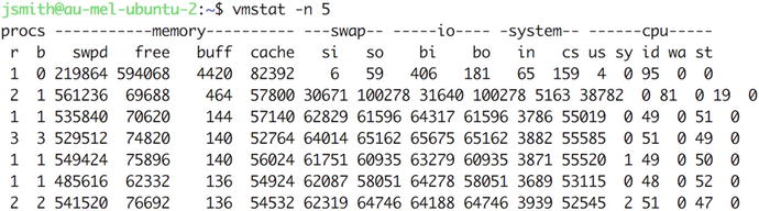
Figure 17-3. vmstat output on heavily swapping host

This rather impressive jumble of numbers gives us an indication of how much data is moving through the system. Each line consists of sets of numbers in six groups, which provide information on processes, memory, swap, input/output, system, and CPU.

Reduced performance due to excessive swap space usage will show up in two of these groups: swap and cpu.

The si and so columns in the swap group display the amount of swap memory that is being read from (si—swap in) and written to (so—swap out) your swap space. The wa and sy columns in the cpu group tell you the percentage of time the CPU is waiting for data to process system (or kernel) requests—and thus not processing system instructions.

If a host is spending most of its CPU cycles moving applications from and to swap space, the si and so column values will be high. The actual values will depend on the amount of swapping that is occurring and the speed of your swap device. The wa column will usually display values in the high 90s as well, indicating the CPU is waiting for an application or data to be retrieved from swap space.

You can solve this problem by using top to find out which application is using too much RAM and possibly changing its configuration to use less. Mostly you will see your main application is the one using the most memory. In that case, either allocate or install more memory to your system.

procs - ---------memory------------- ---swap-- ---io--- --system-- ------cpu-----
 r  b   swpd   free     buff  cache   si   so    bi    bo    in    cs     us sy id wa st
 0  0   422336 750352   8252 130736    0    0     0     0     27   56     0  0 100  0  0
 0  0   422332 750352   8252 130736    1    0     1     0     27   55     0  0 100  0  0

In the previous example, this is an example of a host under light load. This host has low swap space, and the CPU spends most of its time idle.

Disk Access

The vmstatutility will also give us information on how much data is being read from and written to disk. We’ve highlighted the bi (blocks in) and bo (blocks out) columns in the io group in Figure 17-4. By passing a second number as a parameter, we’ve told vmstat to quit after five intervals.

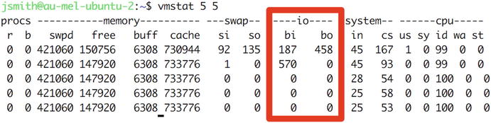
Figure 17-4. vmstat with low disk I/O

These two numbers tell you exactly how many blocks of data are being read from (bi) and written to (bo) your disks during each interval. In our case, the system is reading more data from disk than it is writing back, but both numbers are low. Because the block size on our disks is 4KB, this means they aren’t very heavily loaded.

What constitutes a heavy load will depend on the block size and the speed of the disks. If a large file is being written, this number will go up for the duration of the write operation but drop down again later.

You can get an idea of what your host is capable of by checking the numbers you get when creating a large file on an otherwise idle system. Run a dd command to create a 1Gb file containing only zeroes in the background, while running vmstat simultaneously, as shown in Figure 17-5.

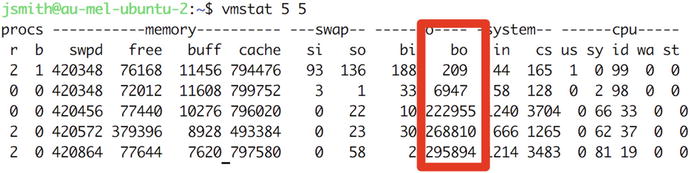
Figure 17-5. vmstat with high disk I/O

On the same host we will run the following command:

$ dd if=/dev/zero of=./largefile bs=1M count=1024

Then when we run the vmstat command at the same time, you will see something similar to Figure 17-5.

The bo column is low for the two runs, as the file data is still in the kernel buffer. At the next interval, however, you can see it spike to more than 222,000 blocks. Keep in mind that this is over 5 seconds, though, so we can calculate the peak write rate on this particular host to be around 45,000 blocks per second.

If you notice degraded performance and vmstat shows a bo value that is up near the maximum rate that the system could manage when you tested it for a long time, you have an application or service that is trying very hard to write a lot of data. This usually indicates a problem, so you should find out which application is the culprit and rectify the problem.

Deeper with dstat

How could you find out which application might have a problem? The vmstat command is great to see a problem, but it doesn’t allow you to go deeper in your investigations. The dstat command, on the other hand, is a great tool at digging.

You can install dstat via the dstat package on both Ubuntu and CentOS using the package manager YUM or Apt. Once one is installed, you can issue the output shown in Figure 17-6.

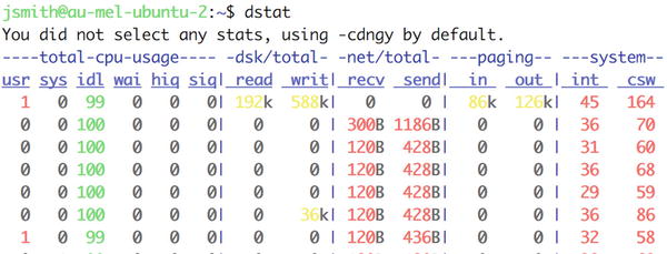
Figure 17-6. dstat output

So far it’s not that much different from vmstat, except that we have disk reads and writes calculated for us, and we also we have network send and receive information. The CPU, paging, and system are the same as vmstat.

Let’s suppose that we have noticed that our application is performing poorly and we think it is due to disk performance. When we look at vmstat, we see the results in Figure 17-7.

Figure 17-7. Checking I/O with vmstat

We can see that we have a fair bit of data being written (bo), but we have no idea to what disk. With our pretend application, we have three partitions that are mounted to /app/log, /app/sys, and /app/data. The partitions are sdc1, sdb1, and sdb2 respectively. We will use this information to see what dstat says.

In Figure 17-8 we can see that we have used the –D switch to dstat to pass in the partitions we want to monitor. We have a significant amount of data being written to sdc1, which is our application logging. In our pretend world I would suspect that our application has been started with debug logging.

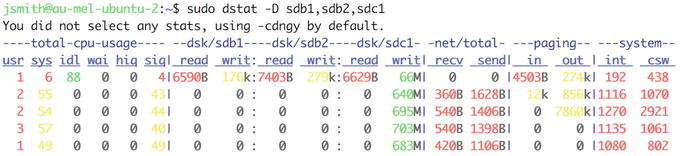
Figure 17-8. dstat disk access

Similarly, you can use the –N switch to supply network interfaces to dstat (-N em1,em2) to report network traffic per interface. The –C will do a similar job for CPUs. You should check the help or man page for more information.

We’ll come back to how you can get notifications when system performance degrades when we cover Nagios in Chapter 18.

Collectd

Collectd is a robust system metrics collection daemon that can collect information about your system and various applications and services. It is highly configurable and works out of the box to collect metrics for you.

We are going to use Collectd to gather metrics from our hosts and send them to Graphite, a metrics collection store. However, you can write metrics to many other back ends using the Write HTTP or Network plug-in.

You can install Collectd on both Ubuntu and CentOS via your package manager. For CentOS you will need to have the epel-release package installed as the Collectd packages aren’t available in the standard repositories.

The Ubuntu version available from the standard Ubuntu repositories is slightly behind the current version, but the CentOS version is fairly recent; depending on the features you require, this may affect your install decisions.

Installation is simple. On CentOS you would issue the following to install Collectd and the mysql plug-in:

$ sudo yum install collectd collectd-mysql

There are several plug-in packages that you can install in the same way, depending on your requirements (use yum search collectd for a list). On Ubuntu it is simply as follows:

$ sudo aptitude install collectd

global options

# plugin without options
LoadPlugin plugin_name
# loading a plugin and overriding options
<LoadPlugin plugin_name>
    ...plugin options...
</LoadPlugin>
# provide an option block to plugins without a LoadPlugin stanza (requires AutoLoadPlugin true)
<Plugin plugin_name>
    ... plugin options...
</Plugin>

#Hostname "localhost"
FQDNLookup true
#BaseDir "/var/lib/collectd"
#PluginDir "/usr/lib/collectd"
#TypesDB "/usr/share/collectd/types.db" "/etc/collectd/my_types.db"
#AutoLoadPlugin false
#CollectInternalStats false
#Interval 10
#MaxReadInterval 86400
#Timeout         2
#ReadThreads     5
#WriteThreads    5
#WriteQueueLimitHigh 1000000
#WriteQueueLimitLow   800000

LoadPlugin syslog
<Plugin syslog>
    LogLevel info
</Plugin>

LoadPlugin cpu
LoadPlugin df
LoadPlugin disk
LoadPlugin interface
LoadPlugin load
LoadPlugin memory
LoadPlugin mysql
LoadPlugin swap
LoadPlugin rrdtool

<Plugin cpu>
    ReportByCpu true
    ReportByState true
    ValuesPercentage false
</Plugin>

<Plugin df>
    FSType rootfs
    FSType sysfs
    FSType proc
    FSType devtmpfs
    FSType devpts
    FSType tmpfs
    FSType fusectl
    FSType cgroup
    IgnoreSelected true
</Plugin>

<Plugin disk>
    Disk "/^(xv)?[hs]?d[a-z]d?$/"
    IgnoreSelected false
    UseBSDName false
    UdevNameAttr "DEVNAME"
</Plugin>

/dev/sda2
/dev/hdb4
/dev/xvda3

<Plugin interface>
    Interface "localhost"
    IgnoreSelected true
</Plugin>

<Plugin load>
    ReportRelative true
</Plugin>

<Plugin memory>
    ValuesAbsolute true
    ValuesPercentage false
</Plugin>

<Plugin mysql>
    <Database no_db>
        Host "localhost"
        Port "3306"
        User “monitor"
        Password “monitorpasswd"
        ConnectTimeout 10
        InnodbStats true
    </Database>
</Plugin>

<Plugin rrdtool>
    DataDir "/var/lib/collectd/rrd"
    CacheTimeout 120
    CacheFlush 900
    WritesPerSecond 30
    CreateFilesAsync false
    RandomTimeout 0
</Plugin>

<Include "/etc/collectd/collectd.conf.d">
    Filter "*.conf"
</Include>

$ sudo systemctl start collectd
$ sudo systemctl status collectd
$ sudo systemctl enable collectd

-- Unit collectd.service has begun starting up.
Nov 15 21:55:26 backup collectd[8000]: plugin_load: plugin "syslog" successfully loaded.
Nov 15 21:55:26 backup collectd[8000]: plugin_load: plugin "cpu" successfully loaded.
Nov 15 21:55:26 backup collectd[8000]: plugin_load: plugin "interface" successfully loaded.
Nov 15 21:55:26 backup collectd[8000]: plugin_load: plugin "load" successfully loaded.
Nov 15 21:55:26 backup collectd[8000]: plugin_load: plugin "memory" successfully loaded.
Nov 15 21:55:26 backup collectd[8000]: plugin_load: plugin "mysql" successfully loaded.
Nov 15 21:55:26 backup collectd[8000]: plugin_load: plugin "rrdtool" successfully loaded.
Nov 15 21:55:26 backup collectd[8000]: Systemd detected, trying to signal readyness.
Nov 15 21:55:26 backup collectd[8000]: Initialization complete, entering read-loop.
Nov 15 21:55:26 backup systemd[1]: Started Collectd statistics daemon.
-- Subject: Unit collectd.service has finished start-up
-- Defined-By: systemd
-- Support: http://lists.freedesktop.org/mailman/listinfo/systemd-devel
--
-- Unit collectd.service has finished starting up.
--
-- The start-up result is done.
Nov 15 21:55:26 backup collectd[8000]: mysql plugin: Successfully connected to database <none> at server Localhost via UNIX socket with cipher <none> (server version: 5.5.50-MariaDB, protocol version: 10)

Graphite

According to the web site, Graphite does only three things: kicks arse, chews bubble gum, and makes it easy to store and graph metrics. We are unqualified to verify the first two statements, but the third statement is correct.

There are four components to Graphite.

• Carbon: A high-performance listener for receiving time-series data

• Whisper: A time-series database for metrics data

• Graphite-web: A web UI that renders graphs and dashboards

• Graphite-API: An API that fetches JSON data from the time-series Whisper database

In this exercise we are going to be installing Carbon, the time-series Whisper database and the Graphite-API. We will be using Grafana to display our metrics (in the next section) and so do not need install Graphite-web.

The Carbon components are comprised of carbon-relays and carbon-aggregators and carbon-cache. We are interested in installing the carbon-cache and a carbon-relay. All three components help to scale the Carbon service to enable the collection of thousands of metrics per second.

The carbon-cache is a required component and forms the basic collection model, carbon-cache, Whisper, and Graphite-API. It is able to listen on UDP or TCP ports (2003, 2004, 2007) and supports Python pickle and newline-delimited formats. The carbon-cache also configures how data will be stored in the Whisper databases. You can store different retention periods based on certain metric patterns. These are referred to as the storage-schema.

The carbon-relay is used to send metrics to certain back-end servers based on metric patterns. There are two ways a carbon-relay can be used, for sharding requests (using consistent hashing) to multiple backends and for replication, sending metrics to any number of different carbon-cache servers or aggregators.

Carbon-aggregators are used to buffer metrics that are destined for the carbon-cache to help reduce I/O. Averages or sums can be made of the metrics and pushed into Whisper as a single metric, reducing I/O on the carbon-cache and Whisper database.

Whisper is a time-series database for long-term storage of your metrics data. It is written in Python and allows for high-precision data resolution to degrade over time. When data degrades, the data points are “rolled up” or aggregated. You can choose to aggregate using the following functions:

• Average (default)

• Sum

• Max

• Min

• Last

You can find more information on Whisper here:

• http://graphite.readthedocs.io/en/latest/whisper.html

Graphite-web is one of the ways you can view your data. It is a Python app that requires the backing of a database, either SQLite (for very small deployments), MariaDB, or PostgreSQL. It also supports LDAP authentication.

If you want to present your metrics via a different graphical presentation service, you can just install Graphite-API , which will return JSON responses to metric queries. This provides a lighter, stateless interface into your metrics from any number of third-party graphical web UIs.

$ sudo yum install -y python-carbon

$ sudo yum install –y graphite-api

$ sudo aptitude install -y graphite-carbon

$ sudo aptitude install –y graphite-api

[cache]
STORAGE_DIR    = /var/lib/graphite/
LOCAL_DATA_DIR = /var/lib/graphite/whisper/
CONF_DIR       = /etc/carbon/
LOG_DIR        = /var/log/carbon/
PID_DIR        = /var/run/
ENABLE_LOGROTATION = False
USER = _graphite

ENABLE_UDP_LISTENER = False
UDP_RECEIVER_INTERFACE = 0.0.0.0
MAX_CACHE_SIZE = inf
MAX_UPDATES_PER_SECOND = 500
MAX_CREATES_PER_MINUTE = 50
CACHE_WRITE_STRATEGY = sorted
WHISPER_AUTOFLUSH = False
WHISPER_FALLOCATE_CREATE = True
USE_FLOW_CONTROL = True
LOG_LISTENER_CONNECTIONS = True
LOG_UPDATES = False
LOG_CACHE_HITS = False
LOG_CACHE_QUEUE_SORTS = True
USE_INSECURE_UNPICKLER = False

LINE_RECEIVER_INTERFACE = 0.0.0.0
PICKLE_RECEIVER_INTERFACE = 0.0.0.0
CACHE_QUERY_INTERFACE = 0.0.0.0
LINE_RECEIVER_PORT = 2003
PICKLE_RECEIVER_PORT = 2004
CACHE_QUERY_PORT = 7002

[cache:1]
LINE_RECEIVER_PORT = 2103
PICKLE_RECEIVER_PORT = 2104

[carbon]
pattern = ^carbon.
retentions = 60s:90d

[default_1min_for_1day]
pattern = .*
retentions = 60s:1d

carbon.agents.host1.cache.queries

[database_metrics]
pattern = ^collectd_(db|backup)_*
retentions = 15s:7d,1m:90d,15m:180d

[cache]
STORAGE_DIR    = /var/lib/graphite/
LOCAL_DATA_DIR = /var/lib/graphite/whisper/
CONF_DIR       = /etc/carbon/
LOG_DIR        = /var/log/carbon/
PID_DIR        = /var/run/
ENABLE_LOGROTATION = False
USER = carbon
LOG_LISTENER_CONNECTIONS = True
USE_INSECURE_UNPICKLER = False
USE_FLOW_CONTROL = True
CACHE_WRITE_STRATEGY = sorted

[relay]
LINE_RECEIVER_INTERFACE = 0.0.0.0
PICKLE_RECEIVER_INTERFACE = 0.0.0.0
LINE_RECEIVER_PORT = 2013
PICKLE_RECEIVER_PORT = 2014
DESTINATIONS = monitor.example.com:2004
LOG_LISTENER_CONNECTIONS = True
RELAY_METHOD = rules
MAX_DATAPOINTS_PER_MESSAGE = 500
MAX_QUEUE_SIZE = 10000
QUEUE_LOW_WATERMARK_PCT = 0.8
USE_FLOW_CONTROL = True

[default]
default = true
destinations = monitor.example.com:2004

[backup_example]
pattern = ^collectd_backup_example_com.*
destination = 192.168.0.250:2004
continue = true

$ sudo systemctl start carbon-relay

$ sudo systemctl start carbon-relay@default

LoadPlugin write_graphite

<Plugin write_graphite>
  <Node "monitor">
    Host "relay.example.com"
    Port "2013"
    Protocol "tcp"
    ReconnectInterval 0
    LogSendErrors true
    Prefix "collectd_"
    StoreRates true
    AlwaysAppendDS false
    EscapeCharacter "_"
  </Node>
</Plugin>

$ sudo getsebool collectd_tcp_network_connect
collectd_tcp_network_connect --> off
$ sudo setsebool collectd_tcp_network_connect on

Nov 22 23:19:06 backup collectd[5999]: plugin_load: plugin "write_graphite" successfully loaded.

22/11/2016 12:29:56 :: MetricLineReceiver connection with 192.168.0.30:38309 established

20/11/2016 10:19:03 :: MetricPickleReceiver connection with 192.168.0.251:52146 established

21/11/2016 11:35:48 :: new metric collectd_backup_example_com.cpu-0.cpu-user matched schema default_1min_for_1day

$ sudo pip3 install gunicorn

$ ln –s /usr/local/bin/gunicorn /usr/bin/gunicorn

[Unit]
Description=graphite-api socket

[Socket]
ListenStream=/run/graphite-api.sock
ListenStream=127.0.0.1:8881

[Install]
WantedBy=sockets.target

[Unit]
Description=Graphite-API service
Requires=graphite-api.socket

[Service]
ExecStart=/usr/bin/gunicorn -b 127.0.0.1:8881 -w2 graphite_api.app:app
Restart=on-failure
ExecReload=/bin/kill -s HUP $MAINPID
ExecStop=/bin/kill -s TERM $MAINPID
PrivateTmp=true

[Install]
WantedBy=multi-user.target

$ sudo systemctl start graphite-api.service

upstream graphite {
    server 127.0.0.1:8881 fail_timeout=0;
}

server {
    server_name monitor;
    listen 80;
    root /var/www;

    location / {
        try_files $uri @graphite;
    }

    location @graphite {
        proxy_pass http://graphite;
    }
}

$ sudo ln –s /etc/nginx/sites-available/graphite.conf /etc/nginx/sites-enabled/graphite.conf
$ sudo systemctl start nginx

$ sudo systemctl start nginx

$ curl -H 'Host: monitor' http://127.0.0.1:80/metrics/find?query=*
[{"text": "carbon", "expandable": 1, "allowChildren": 1, "id": "carbon", "leaf": 0}, {"text": "relay", "expandable": 1, "allowChildren": 1, "id": "relay", "leaf": 0}]

Grafana

Grafana is a visualization web application for graphing time-series data. It can talk to a variety of data sources including Graphite-API. With your newly created metrics, you can now create dashboards and display those metrics.

Grafana supports LDAP authentication and can use a database to store users’ dashboards. It has a stand-alone web service that you interact with. You can install it on your localhost or a central server; it does not store metric data locally but will make request to back-end storage services, in our case Graphite.

Installing Grafana

We are going to install Grafana on our Ubuntu server. We are going to follow the instructions from here: http://docs.grafana.org/installation/debian . You can follow the instructions here for CentOS: http://docs.grafana.org/installation/rpm/ . You can also install Grafana on macOS or Windows.

First we will add the Grafana repository.

$ sudo bash -c 'echo "deb https://packagecloud.io/grafana/stable/debian/ jessie main" > /etc/apt/sources.list.d/grafana.list'
$ curl https://packagecloud.io/gpg.key | sudo apt-key add -
$ sudo aptitude update
$ sudo aptitude install –y grafana

Once it is installed, we can start the Grafana service. This is the same for both Ubuntu and CentOS:

$ sudo systemctl start grafana-server

Now we can access Grafana on the following URL: http://monitor:3000. By default the username and password are admin (Figure 17-9).

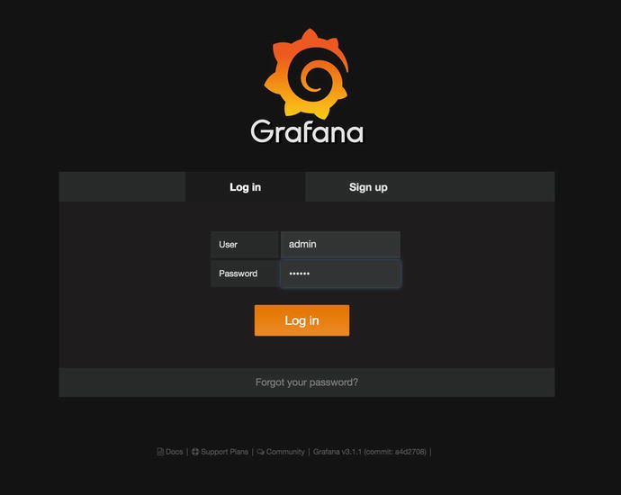
Figure 17-9. Logging into Grafana

Adding Storage Back End

Before we can graph any of our newly Collectd metrics, we need to add our Graphite back end. We need to add it as a data source (Figure 17-10).

Figure 17-10. Selecting data sources

From the Data Sources screen we click the green “Add data source ” button and fill in the details (Figure 17-11).

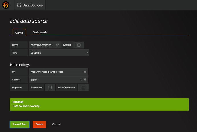
Figure 17-11. Adding Graphite as our data source

Clicking Save & Test will try to make a request to our Graphite host and test that it can get appropriate data back. If we click the Dashboards tab, we will import the Graphite metrics dashboard (Figure 17-12).

Figure 17-12. Clicking Import

After you have imported the dashboard, you can click Graphite Carbon Metrics and you will be shown Figure 17-13.

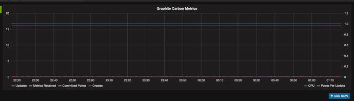
Figure 17-13. Carbon Metrics graph

Let’s create a new dashboard by selecting Create New , as shown in Figure 17-14.

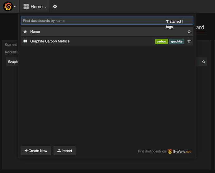
Figure 17-14. Creating a new graph

When you create a dashboard, a green bar will appear on the left side. Then select Add Panel and Graph, as shown in Figure 17-15.

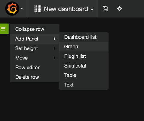
Figure 17-15. From the left drop-down, select Graph

When you add a panel, you get a test metric graph based on fake data (Figure 17-6).

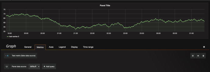
Figure 17-16. Test metric

To create our own graphs, we have to select the data source first. Let’s do that, as in Figure 17-17.

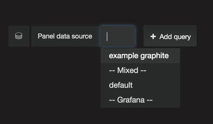
Figure 17-17. Selecting the Panel data source

Once we select the data source , the test data will disappear. You can click “select metric” and choose the origin of the metric you want to graph. We have selected “collectd_backup_example_com,” and then we can select the metrics we interested in. We will choose “load” out of the list. We then select all the metrics available (*) and then again (*). In Figure 17-18 you can see we have tracked the host’s load over 15 minutes. You can see more about Grafana in this YouTube tutorial by Grafana: https://youtu.be/1kJyQKgk_oY .

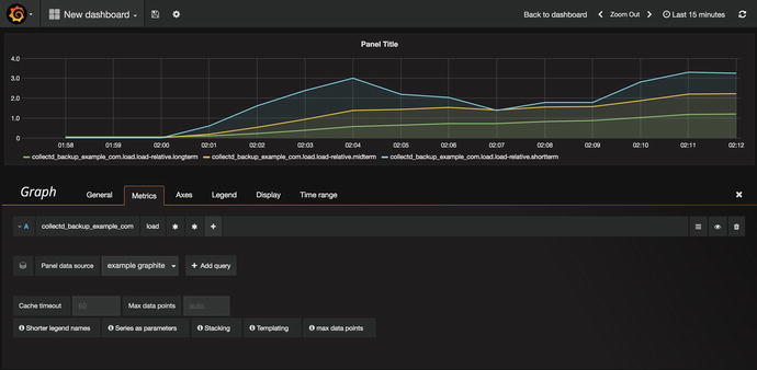
Figure 17-18. Seeing load metrics on backup host

Now that you have your metrics being collected and discoverable, you look at making performance tweaks and be able to measure their effect.

Resource Limits

Linux allows you to enforce resource limits on users via the ulimit command . This is actually a built-in function of the Bash shell . Any limits you set via this command apply only to the current shell and the processes it starts.

To report current limits, run ulimit with the -a option, as shown in Figure 17-19.

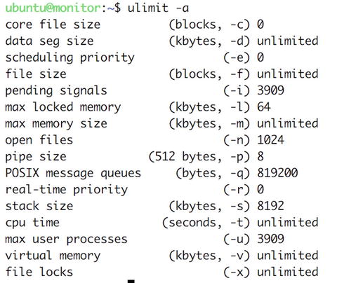
Figure 17-19. ulimit -a

To prevent a fork bomb from being run by this shell user, you can change the maximum number of running processes, for instance, from 3909 to 1, using the -u option. If you then try to run a new process, the system will prevent you from doing so.

$ ulimit -u 1
$ ls
bash: fork: Resource temporarily unavailable

You receive an error to indicate the shell could not fork the command you tried to run. We are not suggesting that you manage users in this way but instead demonstrating the effect of this command.

The other useful limits are the maximum memory size, which can be set via the -m option, and the number of open files, which you set via -n. The most common change you may make when tuning for resource limits is the number of open files a user can have.

You can obtain a full listing of options and their functions in the ulimit section of the man bash page.

Setting Limits for All Users

The ulimit command sets limits for the current shell, so you can add limits via /etc/profile or /etc/bashrc for users who log in. However, most daemons don’t use shells, so adding limits to the shell configuration files won’t have any effect.

You can instead use the limits module for PAM. This module is invoked when a user creates a new process, and it sets limits that you can define in /etc/security/limits.conf. This file defines both soft and hard limits for users and groups. We’ve included the sample limits.conf from CentOS in Figure 17-20.

Figure 17-20. Setting limits for all users

Each line specifies a domain that the limit applies to. This domain can be a wildcard, a username, or a group name. Next comes the limit type, which can be either soft or hard. A hard limit can be set only by the root user, and when a user or process tries to break this limit, the system will prevent this. The soft limit can be adjusted by the user using the ulimit command, but it can be increased only to the value of the hard limit.

Next is the resource that is being limited. A full listing of available resources is included in the sample file, and it also available on the man limits.conf page. Last on each line is the value that the limit should be set to. Lines beginning with # are comments or examples.

In the case of the sample file, the @faculty group is allowed to run 20 concurrent processes (nproc) according to their soft limit. However, any member of this group is allowed to change that limit to any value up to 50 but no higher than that.

sysctl and the proc File System

We briefly mentioned the proc file system in Chapter 9 as a way to obtain system information directly from the kernel. It also provides a way to tweak a running kernel to improve system performance. To this end, you can change values in virtual files under the /proc/sys directory.

The virtual files are grouped in subdirectories, based on the parts of the system they affect, as listed in Table 17-2.

We won’t go into detail on every single file, but we’ll give you an idea of the kinds of tweaking that can be done.

Each of the virtual files contains one or more values that can be read via cat or the sysctlutility. To list all current settings, we can use the following:

$ sysctl –a
abi.vsyscall32 = 1
crypto.fips_enabled = 0
debug.exception-trace = 1
debug.kprobes-optimization = 1
dev.hpet.max-user-freq = 64
dev.mac_hid.mouse_button2_keycode = 97
...
vm.percpu_pagelist_fraction = 0
vm.stat_interval = 1
vm.swappiness = 30
vm.user_reserve_kbytes = 29608
vm.vfs_cache_pressure = 100
vm.zone_reclaim_mode = 0

To read a particular value, pass its key as a parameter to sysctl.

$ sudo sysctl vm.swappiness
vm.swappiness = 30

The key is the full path to the file, with /proc/sys/ removed and the slashes optionally replaced with full stops. For instance, to check how likely your host is to use swap memory, you can check the contents of /proc/sys/vm/swappiness.

$ cat /proc/sys/vm/swappiness
30

This particular value is an indication of how likely the kernel is to move information from RAM into swap space after it hasn’t been used for a while. The higher the number, the more likely this is. The value in this case can range from 0 to 100, with 60 being the default. If you wanted to ensure your host is less likely to use swap memory, you could set the value to 20 instead via the sysctl utility and the -w option. You would need to then pass the key whose value you want to change and the new value.

$ sudo sysctl -w vm.swappiness=20

Another example is the number of files and directories that can be open at any single moment on the system. This is defined in /proc/sys/fs/file-max, and you can read the value via the command sysctl fs.file-max. To increase the maximum number of open files to half a million, run sudo sysctl -w fs.file-max=500000.

When the system is rebooted, these variables are reset to their default values. To make them persist, you can add an appropriate entry in the /etc/sysctl.conf file. When the system boots, all settings in this file are applied to the system via the sysctl -p command.

On Ubuntu , instead of directly editing /etc/sysctl.conf, you can create a file in /etc/sysctl.d/<number>-<option-name>.conf, and they will be read in at boot.

On CentOS you will find the default system settings in /usr/lib/sysctl.d. You can override these in /etc/systctl.conf or by placing a file like on Ubuntu in /etc/sysctl.d/.

More information on sysctl settings can be found with man sysctl.d. A comprehensive list of available variables, with documentation, is available at https://www.kernel.org/doc/Documentation/sysctl/ .

Storage Devices

In Chapter 9 you saw that in the event of a disk failure, the kernel needs to rebuild the RAID array once a replacement disk is added. This task generates a lot of I/O and can degrade performance of other services that the machine may be providing. Alternatively, you might want to give priority to the rebuild process, at the expense of services.

While a rebuild occurs, the kernel keeps the rebuild speed between set minimum and maximum values. We can change these numbers via the speed_min_limit and speed_max_limit entries in the /proc/sys/dev/raid directory.

A more acceptable minimum speed would be 20,000K per second per disk, and you can set it using sysctl.

$ sudo sysctl -w dev.raid.speed_limit_min=20000

Setting the minimum too high will adversely affect performance of the system, so make sure you set this number lower than the maximum throughput the system can handle, divided by the number of disks in your RAID array.

The maximum, which can be changed by setting the dev.raid.speed_limit_max variable, is fairly high already. If you want a RAID rebuild to have less of a performance impact, at the cost of a longer wait, you can lower this number.

To make these changes permanent, add these key-value pairs to /etc/sysctl.conf.

File System Tweaks

Each time a file or directory is accessed, even if it’s only for reading, its last accessed time stamp (or atime) needs to be updated and written to the disk. Unless you need this timestamp, you can speed up disk access by telling your host to not update these.

By default, your system should mount your disks with the relatime option. This option means that each file access does not initiate an update to the file metadata, which increases performance by not issuing unnecessary operations. It is synonymous with noatime.

If it is not set, you simply add the noatime option to the options field in the /etc/fstab file for each filesystem on which you want to enable this option.

UUID=f87a71b8-a323-4e8e-acc9-efb0758a0642 / ext4 defaults,
   errors=remount-ro,relatime 0 1

This will enable the option the next time the filesystem is mounted. To make it active immediately, you can remount the filesystem using the mount command.

$ sudo mount -o remount,relatime /

In addition to mount options, filesystems themselves provide some features that may improve performance; these vary depending on what a particular file system is used for. The main one of these is dir_index, and it applies to the ext2, ext3, and ext4 file systems. Enabling this feature causes the file system to create internal indexes that speed up access to directories containing a large number of files or subdirectories. You can use the tune2fs utility to check whether it’s enabled.

$sudo tune2fs -l /dev/md0 | grep features
Filesystem features: has_journal ext_attr resize_inode dir_index filetype needs_recovery extent 64bit flex_bg
    sparse_super large_file huge_file uninit_bg dir_nlink extra_isize

If you need to change features, and you rarely do, you could use tune2fs to enable a particular feature.

sudo tune2fs -O dir_index /dev/md0

Alternatively, features can be turned off by prefixing their name with a caret.

sudo tune2fs -O ^dir_index /dev/md0

You can set which options should be enabled on the various ext file systems by changing the defaults in the /etc/mke2fs.conf file.

I/O Schedulers

I/O schedulers, also called I/O elevators, are algorithms that kernel will use to order I/O to disk subsystems. Schedulers can be changed to improve the efficiency of this process. Three schedulers are available to the kernel.

• Cfq: This is the default scheduler for SATA devices and tries to implement completely fair queues for processing I/O.

• Deadline: This is the default scheduler for block devices. It preferences read requests and tries to provide certainty to requests by imposing a deadline on the start time.

• Noop: This is a first in/first out queue, where the I/O is left to lower subsystems to order; it is suitable for virtual machines.

You can find the scheduler on your device by executing a command similar to this:

$ cat /sys/block/sda/queue/scheduler
noop deadline [cfq]

The scheduler in [] is the current setting. You can change it with the following command:

$ sudo bash -c  'echo deadline > /sys/block/sda/queue/scheduler'
$ cat /sys/block/sda/queue/scheduler
noop [deadline] cfq

You can set the scheduler at boot time by making an edit to GRUB. You will need to edit the following file by adding this:

$ vi /etc/default/grub
GRUB_CMDLINE_LINUX="console=tty0 ... rhgb quiet elevator=deadline"

This sets deadline as the default scheduler across the whole server. You then need to remake GRUB with the following:

$ sudo grub2-mkconfig -o /boot/grub2//grub.cfg

Now when you reboot your host, the default scheduler is deadline.

$ cat /sys/block/sda/queue/scheduler
noop [deadline] cfq

Remember that on Ubuntu grub2-mkconfig needs to be like this:

$ sudo grub2-mkconfig -o /boot/grub/grub2.cfg

Now your changes will persist across reboots.