
Chapter 5
Understanding the Tools
IN THIS CHAPTER
![]() Working with the Jupyter console
Working with the Jupyter console
![]() Working with Jupyter Notebook
Working with Jupyter Notebook
![]() Interacting with multimedia and graphics
Interacting with multimedia and graphics
Up to this point, the book spends a lot of time working with Python to perform data science tasks without actually engaging the tools provided by Anaconda much. Yes, a good deal of what you do involves typing in code and seeing what happens. However, if you don’t actually know how to use your tools well, you miss opportunities to perform tasks easier and faster. Automation is an essential part of performing data science tasks in Python.
This chapter is about working with the two main Anaconda tools, Jupyter console and Jupyter Notebook. Earlier chapters give you some experience with both tools, but those chapters don’t explore either tool in any detail, and you need to know these tools a lot better for upcoming chapters. The skills you develop in this chapter will help you perform tasks in later chapters with greater speed and far less effort.
The chapter also looks at tasks you can perform with your newfound skills. You develop even more skills as the book progresses, but these tasks help put your new skills into perspective and appreciate how you can use them to make working with Python even easier.
 You don’t have to manually type the source code for this chapter. In fact, it’s a lot easier if you use the downloadable source. The source code for this chapter appears in the
 P4DS4D2_05_Understanding the Tools.ipynb source code file. (See the Introduction for details on where to locate this file.)
Using the Jupyter Console
The Python console (accessible through the Anaconda Prompt) is where you can experiment with data science interactively. You can try things and see the results immediately. If you make a mistake, you can simply close the console and create a new one. The console is for playing around and considering what might be possible. The following sections help you understand what you can do to make your Jupyter console experience better.
The standard Python console that comes with a downloaded copy of Python and the Anaconda version of the Python console (accessed with the IPython command) look similar, and you can perform many of the same tasks using them. (From this point on, the Anaconda version of the Python console appears simply as the IPython console in the text for the sake of simplicity.) If you already know how to use the standard Python console, you have an advantage when it comes to working with the IPython console. However, they also have differences. The IPython console provides enhancements that don’t come with the standard Python console. In addition, performing certain tasks, such as pasting large amounts of text, differs between the two consoles, so even if you know how to use the standard Python console, reading the sections that follow will help you.
Interacting with screen text
When you first start the IPython console by typing ipython at the Anaconda Prompt and pressing Enter, you see a screen similar to the one shown in Figure 5-1. The screen seems loaded with text, but all of it provides useful information. The top line tells you about your version of Python and Anaconda. Below that are three help terms (copyright, credits, and license) that you type to obtain more information about your version of these two products. For example, when you type credits and press Enter, you see a listing of the contributors to this version of the product.

FIGURE 5-1: The opening screen provides information on where to get additional help.
Note that you see a line telling you about enhanced help. If you type ? and press Enter, you see five commands, which you use for the following tasks:
?: Using Jupyter to perform useful workobject?: Discovering facts about the packages, objects, and methods that you use in Python to interact with dataobject??: Obtaining verbose information about the packages, objects, and methods (often pages worth that can become cumbersome to read)%quickref: Obtaining information about the magic functions that Jupyter provideshelp: Learning about the Python programming language (help and ? aren’t the same — the first is for Python and the second is for IPython features)
Depending on your operating system, you should be able to right-click the Anaconda Prompt window and see a context menu containing options for working with the text in the window. Figure 5-2 shows the context menu for Windows. This menu is important because it lets you interact with the text and copy the results of your experimentation in a more permanent form.

FIGURE 5-2: You can cut, copy, and paste text using this context menu.
You can obtain access to the same menu of options by choosing the System menu (click the icon in the upper-left corner of the window) and selecting the Edit menu. The options you commonly see are the following:
- Mark: Selects the specific text you want to copy.
- Copy: Places the text you have marked onto the Clipboard (you can also press Enter after marking the text to perform a copy).
- Paste: Moves text from the Clipboard to the window. Unfortunately, this command doesn’t work right with the IPython console for copying multiple lines of text. Use the
%pastemagic function to copy multiple lines of text instead. - Select All: Performs a mark on all the text visible in the window.
- Scroll: Makes it possible to scroll the window when using the arrow keys. Press Enter to stop scrolling.
- Find: Displays a Find dialog box that you can use to locate text anywhere in the screen buffer. This is actually an exceptionally useful command because you can quickly locate text that you previously entered and want to reuse in some way.
 One feature that the IPython console provides, and that you don’t find when working with the standard Python console, is
 cls, or clear screen. To clear the screen and make typing new commands easier, simply type cls and press Enter. You can also use the following code to reset the shell, similar to restarting the kernel in Notebook:
import IPython
app = IPython.Application.instance()
app.shell.reset()
In this case, the numbering starts over, letting you see the sequence of execution better. If your only goal is to clear variables from memory, use the %reset magic function instead.
Changing the window appearance
The Windows console lets you change the Anaconda Prompt window appearance with ease. Depending on the console and platform you use, you may find that you have other options as well. If your platform doesn’t provide any flexibility in changing the Anaconda Prompt window appearance, you can still do so using a magic function as described in the “Using magic functions” section later in the chapter to change the window appearance. To change the Windows console, click the system menu and choose Properties. You see a dialog box like the one shown in Figure 5-3.

FIGURE 5-3: The Properties dialog box makes it possible to control the appearance of your window.
Each tab controls a different aspect of the window appearance. Even though you’re working with IPython, the underlying console still affects what you see. Here are the purposes for each of the tabs shown in Figure 5-3:
- Options: Determines the size of the cursor (a large cursor works better in bright settings), how many commands the window remembers, and how editing works (such as whether you’re in Insert mode).
- Font: Defines the font used to display text in the window. The Raster Fonts option appears to work best for most people, but trying other font options may help you see the text better under certain conditions.
- Layout: Specifies the window size, position onscreen, and size of the buffer used to hold information that scrolls out of view. If you find that old commands scroll off too quickly, increasing the size of the window can help. Likewise, if you find that you can’t locate older commands, increasing the size of the buffer can help.
- Colors: Determines the basic color settings for the window. The default setting of a black background with gray text is hard for many people to use. Using a white background with black text is much easier. However, you need to choose the color settings that work best for you. These colors are augmented by the colors used by the
%colorsmagic function.
Getting Python help
No one can remember absolutely everything about a programming language. Even the best coders have memory lapses. This is why having language-specific help is so important. Without this help, programmers would spend a great deal of time researching packages, classes, methods, and properties online. Yes, they’ve used them in the past, but they can’t quite bring the required information to mind today.
The Python portion of the IPython console provides two methods of getting help: help mode and interactive help. You use help mode when you want to explore the language and plan to spend some while doing it. Interactive help is better when you know specifically what you need help with and don’t want to spend a lot of time looking at other sorts of information. The following sections tell you how to get help on the Python language whenever you need it.
Entering help mode
To enter help mode, type help( ) and press Enter. The console enters a new mode, in which you can type help-related commands as needed to discover more about Python. You can’t type Python commands in this mode. The prompt changes to a help> prompt, as shown in Figure 5-4, to remind you that you’re in help mode.

FIGURE 5-4: Help mode relies on a special help> prompt.
To obtain help about any object or command, simply type the object or command name and press Enter. You can also type any of the following commands to obtain a listing of other topics of discussion.
modules: Compiles a list of the currently loaded modules. This list varies by how your copy of Python (the underlying language) is configured at any given time, so the list won’t be the same every time you use this command. The command can take a while to execute, and the output list is usually quite large.keywords: Presents a list of Python keywords that you can ask about. For example, you can type assert and learn more about theassertkeyword.symbols: Shows the list of symbols that have special meaning in Python, such as*for multiplication and<<for a left shift.topics: Displays a list of general Python topics, such asCONVERSIONS. The topics appear in uppercase rather than lowercase.
Requesting help in help mode
To obtain help in help mode, you simply type the name of the module, keyword, symbol, or topic that you want to learn more about and press Enter. Help mode is Python specific, which means that you can ask about a list, but not an object based on a list named mylist. You also can’t ask about IPython-specific features, such as the cls command.
When working with features that are part of a module, you need to include the module name. For example, if you want to find out about the version() method within the sys module, you type sys.version and press Enter at the help prompt, rather than just type version.
If a help topic is too large to present as a single screen of information, you see -- More -- at the bottom of the display. Press Enter to advance the help information one line at a time or the spacebar to advance the help information a full screen a time. You can’t go backward in the help listing. Pressing Q (or q) ends the help information immediately.
Exiting help mode
After you finish exploring help, you need to get back to the Python prompt to type more commands. Simply press Enter without entering anything at the help prompt or type quit (without parentheses) and press Enter at the help prompt.
Getting interactive help
Sometimes you don’t want to leave the Python prompt to get help. In this case, you can type help(’<topic>’) and press Enter to obtain help information. For example, to receive help on the print command, you type help(’print’) and press Enter. Notice that the help topic is in single quotation marks. If you try to request help without enclosing the topic in single quotation marks, you see an error message.
Interactive help works with any module, keyword, or topic that Python supports. For example, you can type help(’CONVERSIONS’) and press Enter to receive help about the CONVERSIONS topic. It’s important to note that case is still important when working with interactive help. Typing help(’conversions’) and pressing Enter displays a message telling you that help isn’t available.
Getting IPython help
Getting help with IPython is different from getting help with Python. When you obtain IPython help, you work with the development environment rather than the programming language. To obtain IPython help, type ? and press Enter. You see a long listing of the various ways in which you can use IPython help.
Some of the more essential forms of help rely on typing a keyword with a question mark. For example, if you want to learn more about the cls command, you type cls? or ?cls and press Enter. It doesn’t matter whether the question mark appears before or after the command.
Interestingly enough, you can kick IPython help up a notch. If you want to obtain more details about a command or other IPython feature, use two question marks. For example, ??cls displays the source code for the cls command. The double question mark (??) may not always return additional information if there isn’t any more information to find.
If you want to stop displaying IPython information early, press Q to quit. Otherwise, you can press Space or Enter to display each screen of information until the help system has displayed everything available.
Using magic functions
Amazingly, you really can get magic on your computer! Jupyter provides a special feature called magic functions. The functions let you perform all sorts of amazing tasks with your Jupyter console. The following sections provide an overview of the magic functions. You do see some of them used later in the book as well. However, it pays to spend some time checking out these functions for yourself.
Obtaining the magic functions list
The best way to start working with magic functions is to obtain a list of them by typing %quickref and pressing Enter. What you see is a help screen similar to the one shown in Figure 5-5. The listing can be a little confusing to read, so make sure you take your time with it.

FIGURE 5-5: Take your time going through the magic function help; it has a lot of information.
Working with magic functions
Most magic functions start with either a single percent sign (%) or two percent signs (%%). Those with a single percent sign work at the command-line level, while those that have two percent signs work at the cell level. The Jupyter Notebook discussion later in the chapter talks more about cells. For now, all you really need to know is that you generally use magic functions with a single percent sign within the IPython console.
Most of the magic functions display status information when you use them by themselves. For example, when you type %cd and press Enter, you see the current directory. To change directories, you type %cd plus the new directory location on your system. There are some exceptions to this rule, however. For example, %cls clears the screen when used alone because it doesn’t take any parameters.
One of the more interesting magic functions is %colors. You can use this function to change the colors used to display information onscreen, which is helpful when you use various devices. The available options are NoColor (everything is in black and white), Linux (the default setting), and LightBG (which uses a blue-and-green color scheme). This particular function is another exception to the rule. Typing %colors alone doesn’t display the current color scheme but displays an error message instead.
Discovering objects
Python is all about objects. In fact, you can’t do anything in Python without working with some sort of object. With this in mind, it’s a good idea to know how to discover precisely what object you’re working with and what features it provides. The following sections help you discover the Python objects you use as you code.
Getting object help
With IPython, you can request information about specific objects using the object name and a question mark (?). For example, if you want to know more about a list object named mylist, simply type mylist? and press Enter. You see output showing the mylist type, content in string form, length, and a document string providing a quick overview of mylist.
When you need detailed help about mylist, you type help(mylist) and press Enter instead. You see the same help that you should when requesting information about the Python list. However, you receive the information that’s appropriate to the particular object you need help with, rather than having to first discover the object type and then request information for that object.
Obtaining object specifics
The dir() function is often overlooked, but it’s an essential way to learn about object specifics. To see a list of properties and methods associated with any object, use dir(<object name>). For example, if you create a list called mylist and want to know what sorts of things you can do with it, type dir(mylist) and press Enter. The IPython console displays a list of methods and properties that are specific to mylist.
Using IPython object help
Python provides one level of help about your objects — and IPython provides another. When you want to know more about your object than Python tells you, try using the question mark with it. For example, when working with a list named mylist, you can type mylist? and press Enter to discover the object type, content, length, and associated docstring. The docstring provides you with a quick overview of usage information for the type — enough that you can find more details with what you now know about the object.
Using a single question mark does cause IPython to clip long content. If you want to obtain the full content for an object, you need to use the double question mark (??). For example, type mylist?? and press Enter to see any clipped details (although there may not be any additional details). Whenever possible, IPython provides you with the full source code for the object (assuming that the source code is available).
You can use magic functions with objects as well. These functions simplify the help output and provide only the information you need, as shown here:
%pdoc: Displays thedocstringfor the object%pdef: Shows how to call the object (assuming that the object is callable)%source: Displays the source code for the object (assuming that the source is available)%file: Outputs the name of the file that contains the source code for the object%pinfo: Displays detailed information about the object (often more than provided by help alone)%pinfo2: Displays extra detailed information about the object (when available)
Using Jupyter Notebook
You generally use the IPython console described in previous sections to play with code, and that’s about it. Of course, it works fine for that purpose. However, the Jupyter Notebook Integrated Development Environment (IDE), which is another part of the Anaconda suite of tools, can do more for you. The following sections help you understand some of the interesting things that Jupyter Notebook (simply called Notebook) can help you do.
Working with styles
Here’s one of the ways in which Notebook excels over just about any other IDE that you’ll ever use: It helps you to create nice-looking output. Rather than have a screen full of a whole bunch of plain-old code, you can use Notebook to create sections and add styles so that the output is nicely formatted. What you can end up with is a good-looking report that just happens to contain executable code. The reason for this improved output is the use of styles.
When you type code into Notebook, you place the code in a cell. Each section of code that you create goes into a separate cell. When you need to create a new cell, you click Insert Cell Below (the button with a plus sign) on the toolbar. Likewise, when you decide that you no longer need a cell, you select it and then click Cut Cell (the button with a scissors) to place the deleted cell on the Clipboard, or choose Edit ⇒ Delete Cell to remove it completely.
The default style for a cell is Code. However, when you click the down arrow next to the Code entry, you see a listing of styles, as shown in Figure 5-6.

FIGURE 5-6: Notebook makes adding styles to your work easy.
The various styles shown help you format content in various ways. The Markdown style is most definitely used to separate varies entries. To try it for yourself, choose Markdown from the drop-down list, type the heading for this main chapter section, # Using Jupyter Notebook, in the first cell; next, click Run. The content changes to a heading. The single hash (#) tells Notebook that this is a first-level heading. Notice that clicking Run automatically adds a new cell and places the cursor in it. To add a second-level heading, choose Markdown from the drop-down list, type ## Working with styles, and click Run. Figure 5-7 shows that the two entries are indeed headings and that the second entry is smaller than the first.

FIGURE 5-7: Adding headings makes separating content in your notebooks easy.
The Markdown style also lets you add HTML content, which can contain anything a web page contains with regard to standard HTML tags. Another way to create a first-level heading is to define the cell type as Markdown, type <h1>Using Jupyter Notebook</h1>, and then click Run. In general, you use HTML to provide documentation and links to outside material. Relying on HTML tags makes it possible to include things like lists or even pictures. In short, you can actually include an HTML document fragment as part of your notebook, which makes Notebook much more than a simple means of writing down code.
The use of the Raw NBConvert formatting option is outside the scope of this book. However, it provides you with the means for included information that shouldn’t be modified by the notebook converter (NBConvert). You can output notebooks in a variety of formats, and NBConvert performs this task for you. You can read about this feature at https://nbconvert.readthedocs.io/en/latest/. The goal of the Raw NBConvert style is to allow you to include special content, such as Lamport TeX (LaTeX) content. The LaTeX document system isn’t tied to a particular editor — it’s simply a means of encoding scientific documents.
Restarting the kernel
Every time you perform a task in your notebook, you create variables, import modules, and perform a wealth of other tasks that corrupt the environment. At some point, you can’t really be sure that something is working as it should. To overcome this problem, you click Restart Kernel (the button with an open circle with an arrow at one end) after saving your document by clicking Save and Checkpoint (the button containing a floppy disk symbol). You can then run your code again to ensure that it does work as you thought it would.
Sometimes an error also causes the kernel to crash. Your document starts acting oddly, updates slowly, or shows other signs of corruption. Again, the answer is to restart the kernel to ensure that you have a clean environment and that the kernel is running as it should.
 Whenever you click Restart Kernel, you see the warning message shown in Figure 5-8. Make certain that you pay attention to the warning because you could lose temporary changes during a kernel restart. Always save your document before you restart the kernel.
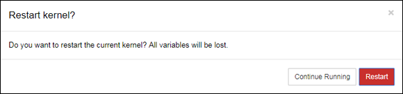
FIGURE 5-8: Save your document before restarting the kernel.
Restoring a checkpoint
At some point, you may find that you made a mistake. Notebook is notably missing an Undo button: You won’t find one anywhere. Instead, you create checkpoints each time you finish a task. Creating checkpoints when your document is stable and working properly helps you recover faster from mistakes.
To restore your setup to the condition contained in a checkpoint, choose File ⇒ Revert to Checkpoint. You see a listing of available checkpoints. Simply select the one you want to use. When you select the checkpoint, you see a warning message like the one shown in Figure 5-9. When you click Revert, any old information is gone and the information found in the checkpoint becomes the current information.

FIGURE 5-9: Revert to a previous notebook setup to undo a mistake.
Performing Multimedia and Graphic Integration
Pictures say a lot of things that words can’t say (or at least they do it with far less effort). Notebook is both a coding platform and a presentation platform. You may be surprised at just what you can do with it. The following sections provide a brief overview of some of the more interesting features.
Embedding plots and other images
At some point, you might have spotted a notebook with multimedia or graphics embedded into it and wondered why you didn’t see the same effects in your own files. In fact, all the graphics examples in the book appear as part of the code. Fortunately, you can perform some more magic by using the %matplotlib magic function. The possible values for this function are: ’gtk’, ’gtk3’, ’inline’, ’nbagg’, ’osx’, ’qt’, ’qt4’, ’qt5’, ’tk’, and ’wx’, each of which defines a different plotting backend (the code used to actually render the plot) used to present information onscreen.
When you run %matplotlib inline, any plots you create appear as part of the document. That’s how Figure 8-1 (see the section about using NetworkX basics in Chapter 8) shows the plot that it creates immediately below the affected code.
Loading examples from online sites
Because some examples you see online can be hard to understand unless you have them loaded on your own system, you should also keep the %load magic function in mind. All you need is the URL of an example you want to see on your system. For example, try %load https://matplotlib.org/_downloads/pyplot_text.py. When you click Run Cell, Notebook loads the example directly in the cell and comments the %load call out. You can then run the example and see the output from it on your own system.
Obtaining online graphics and multimedia
A lot of the functionality required to perform special multimedia and graphics processing appears within Jupyter.display. By importing a required class, you can perform tasks such as embedding images into your notebook. Here’s an example of embedding one of the pictures from the author’s blog into the notebook for this chapter:
from IPython.display import Image
Embed = Image(
'http://blog.johnmuellerbooks.com/' +
'wp-content/uploads/2015/04/Layer-Hens.jpg')
Embed
The code begins by importing the required class, Image, and then using features from it to first define what to embed and then actually embed the image. The output you see from this example appears in Figure 5-10.

FIGURE 5-10: Embedding images can dress up your notebook presentation.
If you expect an image to change over time, you might want to create a link to it instead of embedding it. You must refresh a link because the content in the notebook is only a reference rather than the actual image. However, as the image changes, you see the change in your notebook as well. To accomplish this task, you use SoftLinked = Image(url=’http://blog.johnmuellerbooks.com/wp-content/uploads/2015/04/Layer-Hens.jpg’) instead of Embed.
When working with embedded images on a regular basis, you might want to set the form in which the images are embedded. For example, you may prefer to embed them as PDFs. To perform this task, you use code similar to this:
from IPython.display import set_matplotlib_formats
set_matplotlib_formats('pdf', 'svg')
You have access to a wide number of formats when working with a notebook. The commonly supported formats are ’png’, ’retina’, ’jpeg’, ’svg’, and ’pdf’.
The IPython display system is nothing short of amazing, and this section hasn’t even begun to tap the surface for you. For example, you can import a YouTube video and place it directly into your notebook as part of your presentation if you want. You can see quite a few more of the display features demonstrated at http://nbviewer.jupyter.org/github/ipython/ipython/blob/1.x/examples/notebooks/Part%205%20-%20Rich%20Display%20System.ipynb.