
Chapter 19
Increasing Complexity with Linear and Nonlinear Tricks
IN THIS CHAPTER
![]() Expanding your feature using polynomials
Expanding your feature using polynomials
![]() Regularizing your model
Regularizing your model
![]() Learning from big data
Learning from big data
![]() Using support vector machines and neural network
Using support vector machines and neural network
Previous chapters introduce you to some of the simplest, yet effective, machine learning algorithms, such as linear and logistic regression, Naïve Bayes, and K-Nearest Neighbors (KNN). At this point, you can successfully complete a regression or classification project in data science. This chapter explores even more complex and powerful machine learning techniques including the following: reasoning on how to enhance your data; improving your estimates by regularization; and learning from big data by breaking it into manageable chunks.
This chapter also introduces you to the support vector machine (SVM), a powerful family of algorithms for classification and regression. The chapter touches on neural networks as well. Both SVMs and neural networks can perform the most difficult data problems in data science. Initially introduced a few years ago as a replacement for neural networks, neural networks and tree ensembles have recently overtaken SVMs again (the topic of Chapter 20, “Understanding the Power of the Many”) as the state-of-the-art predictive tool. Neural networks have a long history, but only in the last five years have they improved to the point of becoming an indispensable tool for predictions based on images and text. Given the complexity of both regression and classification using advanced techniques, quite a few pages are devoted to SVM and some to neural networks, but increasing your understanding of both strategies is definitely worth the time and effort.
 You don’t have to type the source code for this chapter manually. In fact, it’s a lot easier if you use the downloadable source (see the Introduction for download instructions). The source code for this chapter appears in the
 P4DS4D2_19_Increasing_Complexity.ipynb source code file. You can also plot some of the complex drawings illustrating SVM algorithms by running the code in the P4DS4D2_19_Representing_SVM_boundaries.ipynb source file.
Using Nonlinear Transformations
Linear models, such as linear and logistic regression, are actually linear combinations that sum your features (weighted by learned coefficients) and provide a simple but effective model. In most situations, they offer a good approximation of the complex reality they represent. Even though they’re characterized by a high bias, using a large number of observations can improve their coefficients and make them more competitive when compared to complex algorithms.
However, they can perform better when solving certain problems if you pre-analyze the data using the Exploratory Data Analysis (EDA) approach. After performing the analysis, you can transform and enrich the existing features by
- Linearizing the relationships between features and the target variable using transformations that increase their correlation and make their cloud of points in the scatterplot more similar to a line.
- Making variables interact by multiplying them so that you can better represent their conjoint behavior.
- Expanding the existing variables using the polynomial expansion in order to represent relationships more realistically (such as ideal point curves, when there is a peak in the variable representing a maximum, akin to a parabola).
Doing variable transformations
An example is the best way to explain the kind of transformations you can successfully apply to data to improve a linear model. The example in this section, and the “Regularizing Linear Models” and “Fighting with Big Data Chunk by Chunk” sections that follow, relies on the Boston dataset. The problem relies on regression, and the data originally has ten variables to explain the different housing prices in Boston during the 1970s. The dataset also has implicit ordering. Fortunately, order doesn’t influence most algorithms because they learn the data as a whole. When an algorithm learns in a progressive manner, ordering can interfere with effective model building. By using seed (to fix a preordinated sequence of random numbers) and shuffle from the random package (to shuffle the index), you can reindex the dataset.
From sklearn.datasets import load_boston
import random
from random import shuffle
boston = load_boston()
random.seed(0) # Creates a replicable shuffling
new_index = list(range(boston.data.shape[0]))
shuffle(new_index) # shuffling the index
X, y = boston.data[new_index], boston.target[new_index]
print(X.shape, y.shape, boston.feature_names)
In the code, random.seed(0) creates a replicable shuffling operation, and shuffle(new_index) creates the new shuffled index used to reorder the data. After that, the code prints the X and y shapes as well as the list of dataset variable names:
(506, 13) (506,) ['CRIM' 'ZN' 'INDUS' 'CHAS' 'NOX' 'RM' 'AGE' 'DIS' 'RAD' 'TAX' 'PTRATIO' 'B' 'LSTAT']
 You can find out more detail about the meaning of the variables present in the Boston dataset by issuing the following command:
 print(boston.DESCR). You see the output of this command in the downloadable source code.
Converting the array of predictors and the target variable into a pandas DataFrame helps support the series of explorations and operations on data. Moreover, although Scikit-learn requires an ndarray as input, it will also accept DataFrame objects.
import pandas as pd
df = pd.DataFrame(X,columns=boston.feature_names)
df['target'] = y
The best way to spot possible transformations is by graphical exploration, and using a scatterplot can tell you a lot about two variables. You need to make the relationship between the predictors and the target outcome as linear as possible, so you should try various combinations, such as the following:
ax = df.plot(kind='scatter', x='LSTAT', y='target', c='b')
In Figure 19-1, you see a representation of the resulting scatterplot. Notice that you can approximate the cloud of points by using a curved line rather than a straight line. In particular, when LSTAT is around 5, the target seems to vary between values of 20 to 50. As LSTAT increases, the target decreases to 10, reducing the variation.

FIGURE 19-1: Nonlinear relationship between variable LSTAT and target prices.
Logarithmic transformation can help in such conditions. However, your values should range from zero to one, such as percentages, as demonstrated in this example. In other cases, other useful transformations for your x variable could include x**2, x**3, 1/x, 1/x**2, 1/x**3, and sqrt(x). The key is to try them and test the result. As for testing, you can use the following script as an example:
import numpy as np
from sklearn.feature_selection import f_regression
single_variable = df['LSTAT'].values.reshape(-1, 1)
F, pval = f_regression(single_variable, y)
print('F score for the original feature %.1f' % F)
F, pval = f_regression(np.log(single_variable),y)
print('F score for the transformed feature %.1f' % F)
The code prints the F score, a measure to evaluate how a feature is predictive in a machine learning problem, both the original and the transformed feature. The score for the transformed feature is a great improvement over the untransformed one.
F score for the original feature 601.6
F score for the transformed feature 1000.2
The F score is useful for variable selection. You can also use it to assess the usefulness of a transformation because both f_regression and f_classif are themselves based on linear models, and are therefore sensitive to every effective transformation used to make variable relationships more linear.
Creating interactions between variables
In a linear combination, the model reacts to how a variable changes in an independent way with respect to changes in the other variables. In statistics, this kind of model is a main effects model.
The Naïve Bayes classifier makes a similar assumption for probabilities, and it also works well with complex text problems.
Even though machine learning works by using approximations and a set of independent variables can make your predictions work well in most situations, sometimes you may miss an important part of the picture. You can easily catch this problem by depicting the variation in your target associated with the conjoint variation of two or more variables in two simple and straightforward ways:
- Existing domain knowledge of the problem: For instance, in the car market, having a noisy engine is a nuisance in a family car but considered a plus for sports cars (car aficionados want to hear that you have an ultra-cool and expensive car). By knowing a consumer preference, you can model a noise level variable and a car type variable together to obtain exact predictions using a predictive analytic model that guesses the car’s value based on its features.
- Testing combinations of different variables: By performing group tests, you can see the effect that certain variables have on your target variable. Therefore, even without knowing about noisy engines and sports cars, you could have caught a different average of preference level when analyzing your dataset split by type of cars and noise level.
The following example shows how to test and detect interactions in the Boston dataset. The first task is to load a few helper classes, as shown here:
from sklearn.linear_model import LinearRegression
from sklearn.model_selection import cross_val_score, KFold
regression = LinearRegression(normalize=True)
crossvalidation = KFold(n_splits=10, shuffle=True,
random_state=1)
The code reinitializes the pandas DataFrame using only the predictor variables. A for loop matches the different predictors and creates a new variable containing each interaction. The mathematical formulation of an interaction is simply a multiplication.
df = pd.DataFrame(X,columns=boston.feature_names)
baseline = np.mean(cross_val_score(regression, df, y,
scoring='r2',
cv=crossvalidation))
interactions = list()
for var_A in boston.feature_names:
for var_B in boston.feature_names:
if var_A > var_B:
df['interaction'] = df[var_A] * df[var_B]
cv = cross_val_score(regression, df, y,
scoring='r2',
cv=crossvalidation)
score = round(np.mean(cv), 3)
if score > baseline:
interactions.append((var_A, var_B, score))
print('Baseline R2: %.3f' % baseline)
print('Top 10 interactions: %s' % sorted(interactions,
key=lambda x :x[2],
reverse=True)[:10])
The code starts by printing the baseline R2 score for the regression; then it reports the top ten interactions whose addition to the mode increase the score:
Baseline R2: 0.716
Top 10 interactions: [('RM', 'LSTAT', 0.79), ('TAX', 'RM', 0.782), ('RM', 'RAD', 0.778), ('RM', 'PTRATIO', 0.766), ('RM', 'INDUS', 0.76), ('RM', 'NOX', 0.747), ('RM', 'AGE', 0.742), ('RM', 'B', 0.738), ('RM', 'DIS', 0.736), ('ZN', 'RM', 0.73)]
The code tests the specific addition of each interaction to the model using a 10 folds cross-validation. (The “Cross-Validating” section of Chapter 18 tells you more about working with folds.) The code records the change in the R2 measure into a stack (a simple list) that an application can order and explore later.
The baseline score is 0.699, so a reported improvement of the stack of interactions to 0.782 looks quite impressive. It’s important to know how this improvement is made possible. The two variables involved are RM (the average number of rooms) and LSTAT (the percentage of lower-status population). A plot will disclose the case about these two variables:
colors = ['b' if v > np.mean(y) else 'r' for v in y]
scatter = df.plot(kind='scatter', x='RM', y='LSTAT',
c=colors)
The scatterplot in Figure 19-2 clarifies the improvement. In a portion of houses at the center of the plot, it’s necessary to know both LSTAT and RM in order to correctly separate the high-value houses from the low-value houses; therefore, an interaction is indispensable in this case.

FIGURE 19-2: Combined variables LSTAT and RM help to separate high from low prices.
Adding interactions and transformed variables leads to an extended linear regression model, a polynomial regression. Data scientists rely on testing and experimenting to validate an approach to solving a problem, so the following code slightly modifies the previous code to redefine the set of predictors using interactions and quadratic terms by squaring the variables:
polyX = pd.DataFrame(X,columns=boston.feature_names)
cv = cross_val_score(regression, polyX, y,
scoring='neg_mean_squared_error',
cv=crossvalidation)
baseline = np.mean(cv)
improvements = [baseline]
for var_A in boston.feature_names:
polyX[var_A+'^2'] = polyX[var_A]**2
cv = cross_val_score(regression, polyX, y,
scoring='neg_mean_squared_error',
cv=crossvalidation)
improvements.append(np.mean(cv))
for var_B in boston.feature_names:
if var_A > var_B:
poly_var = var_A + '*' + var_B
polyX[poly_var] = polyX[var_A] * polyX[var_B]
cv = cross_val_score(regression, polyX, y,
scoring='neg_mean_squared_error',
cv=crossvalidation)
improvements.append(np.mean(cv))
import matplotlib.pyplot as plt
plt.figure()
plt.plot(range(0,92),np.abs(improvements),'-')
plt.xlabel('Added polynomial features')
plt.ylabel('Mean squared error')
plt.show()
To track improvements as the code adds new, complex terms, the example places values in the improvements list. Figure 19-3 shows a graph of the results that demonstrates some additions are great because the squared error decreases, and other additions are terrible because they increase the error instead.
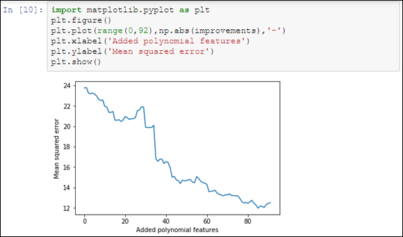
FIGURE 19-3: Adding polynomial features increases the predictive power.
Of course, instead of unconditionally adding all the generated variables, you could perform an ongoing test before deciding to add a quadratic term or an interaction, checking by cross validation if each addition is really useful for your predictive purposes. This example is a good foundation for checking other ways of controlling the existing complexity of your datasets or the complexity that you have to induce with transformation and feature creation in the course of data exploration efforts. Before moving on, you check both the shape of the actual dataset and its cross-validated mean squared error.
print('New shape of X:', np.shape(polyX))
crossvalidation = KFold(n_splits=10, shuffle=True,
random_state=1)
cv = cross_val_score(regression, polyX, y,
scoring='neg_mean_squared_error',
cv=crossvalidation)
print('Mean squared error: %.3f' % abs(np.mean(cv)))
Even though the mean squared error is good, the ratio between 506 observations and 104 features isn’t all that good because the number of observations may not be enough for a correct estimate of the coefficients.
New shape of X: (506, 104)
Mean squared error: 12.514
As a rule of thumb, divide the number of observations by the number of coefficients. The code should have at least 10 to 20 observations for every coefficient you want to estimate in linear models. However, experience shows that having at least 30 of them is better.
Regularizing Linear Models
Linear models have a high bias, but as you add more features, more interactions, and more transformations, they start gaining adaptability to the data characteristics and memorizing power for data noise, thus increasing the variance of their estimates. Trading higher variance for less bias isn’t always the best choice, but, as mentioned earlier, sometimes it’s the only way to increase the predictive power of linear algorithms.
You can introduce L1 and L2 regularization as a way to control the trade-off between bias and variance in favor of an increased generalization capability of the model. When you introduce one of the regularizations, an additive function that depends on the complexity of the linear model penalizes the optimized cost function. In linear regression, the cost function is the squared error of the predictions, and the cost function is penalized using a summation of the coefficients of the predictor variables.
If the model is complex but the predictive gain is little, the penalization forces the optimization procedure to remove the useless variables, or to reduce their impact on the estimate. The regularization also acts on highly correlated features — attenuating or excluding their contribution, thus stabilizing the results and reducing the consequent variance of the estimates:
- L1 (also called Lasso): Shrinks some coefficients to zero, making your coefficients sparse. It performs variable selection.
- L2 (also called Ridge): Reduces the coefficients of the most problematic features, making them smaller, but seldom equal to zero. All coefficients keep participating in the estimate, but many become small and irrelevant.
You can control the strength of the regularization using a hyperparameter, usually a coefficient itself, often called alpha. When alpha approaches 1.0, you have stronger regularization and a greater reduction of the coefficients. In some cases, the coefficients are reduced to zero. Don’t confuse alpha with C, a parameter used by LogisticRegression and by support vector machines, because C is 1/alpha, so it can be greater than 1. Smaller C numbers actually correspond to more regularization, exactly the opposite of alpha.
Regularization works because it is the sum of the coefficients of the predictor variables, therefore it’s important that they’re on the same scale or the regularization may find it difficult to converge, and variables with larger absolute coefficient values will greatly influence it, generating an infective regularization. It’s good practice to standardize the predictor values or bind them to a common min-max, such as the [-1,+1] range. The following sections demonstrate various methods of using both L1 and L2 regularization to achieve various effects.
Relying on Ridge regression (L2)
The first example uses the L2 type regularization, reducing the strength of the coefficients. The Ridge class implements L2 for linear regression. Its usage is simple; it presents just the parameter alpha to fix. Ridge also has another parameter, normalize, that automatically normalizes the inputted predictors to zero mean and unit variance.
from sklearn.model_selection import GridSearchCV
from sklearn.linear_model import Ridge
ridge = Ridge(normalize=True)
search_grid = {'alpha':np.logspace(-5,2,8)}
search = GridSearchCV(estimator=ridge,
param_grid=search_grid,
scoring='neg_mean_squared_error',
refit=True, cv=10)
search.fit(polyX,y)
print('Best parameters: %s' % search.best_params_)
score = abs(search.best_score_)
print('CV MSE of best parameters: %.3f' % score)
After searching for the best alpha parameter, the resulting best model is
Best parameters: {'alpha': 0.001}
CV MSE of best parameters: 11.630
A good search space for the alpha value is in the range np.logspace(-5,2,8). Of course, if the resulting optimum value is on one of the extremities of the tested range, you need to enlarge the range and retest.
The polyX and y variables used for the examples in this section and the sections that follow are created as part of the example in the “Creating interactions between variables” section, earlier in this chapter. If you haven’t worked through that section, the examples in this section will fail to work properly.
Using the Lasso (L1)
The second example uses the L1 regularization, the Lasso class, whose principal characteristic is to reduce the effect of less useful coefficients down toward zero. This action enforces sparsity in the coefficients, with just a few having values above zero. The class uses the same parameters of the Ridge class that are demonstrated in the previous section.
from sklearn.linear_model import Lasso
lasso = Lasso(normalize=True,tol=0.05, selection=’random’)
search_grid = {'alpha':np.logspace(-2,3,8)}
search = GridSearchCV(estimator=lasso,
param_grid=search_grid,
scoring='neg_mean_squared_error',
refit=True, cv=10)
search.fit(polyX,y)
print('Best parameters: %s' % search.best_params_)
score = abs(search.best_score_)
print('CV MSE of best parameters: %.3f' % score)
In setting the Lasso, the code uses a less sensitive algorithm (tol=0.05) and a random approach for its optimization (selection=’random’). The resulting mean squared error obtained is higher than it is using the L2 regularization:
Best parameters: {'alpha': 1e-05}
CV MSE of best parameters: 12.432
Leveraging regularization
Because you can indent the sparse coefficients resulting from a L1 regression as a feature selection procedure, you can effectively use the Lasso class for selecting the most important variables. By tuning the alpha parameter, you can select a greater or lesser number of variables. In this case, the code sets the alpha parameter to 0.01, obtaining a much simplified solution as a result.
lasso = Lasso(normalize=True, alpha=0.01)
lasso.fit(polyX,y)
print(polyX.columns[np.abs(lasso.coef_)>0.0001].values)
The simplified solution is made of a handful of interactions:
['CRIM*CHAS' 'ZN*CRIM' 'ZN*CHAS' 'INDUS*DIS' 'CHAS*B'
'NOX^2' 'NOX*DIS' 'RM^2' 'RM*CRIM' 'RM*NOX' 'RM*PTRATIO'
'RM*B' 'RM*LSTAT' 'RAD*B' 'TAX*DIS' 'PTRATIO*NOX'
'LSTAT^2']
You can apply L1-based variable selection automatically to both regression and classification using the RandomizedLasso and RandomizedLogisticRegression classes. Both classes create a series of randomized L1 regularized models. The code keeps track of the resulting coefficients. At the end of the process, the application keeps any coefficients that the class didn’t reduce to zero because they’re considered important. You can train the two classes using the fit method, but they don’t have a predict method, just a transform method that effectively reduces your dataset, just like most classes in the sklearn.preprocessing module.
Combining L1 & L2: Elasticnet
L2 regularization reduces the impact of correlated features, whereas L1 regularization tends to selects them. A good strategy is to mix them using a weighted sum by using the ElasticNet class. You control both L1 and L2 effects by using the same alpha parameter, but you can decide the L1 effect’s share by using the l1_ratio parameter. Clearly, if l1_ratio is 0, you have a ridge regression; on the other hand, when l1_ratio is 1, you have a lasso.
from sklearn.linear_model import ElasticNet
elastic = ElasticNet(normalize=True, selection='random')
search_grid = {'alpha':np.logspace(-4,3,8),
'l1_ratio': [0.10 ,0.25, 0.5, 0.75]}
search = GridSearchCV(estimator=elastic,
param_grid=search_grid,
scoring='neg_mean_squared_error',
refit=True, cv=10)
search.fit(polyX,y)
print('Best parameters: %s' % search.best_params_)
score = abs(search.best_score_)
print('CV MSE of best parameters: %.3f' % score)
After a while, you get a result that’s quite comparable to L1’s:
Best parameters: {'alpha': 0.0001, 'l1_ratio': 0.75}
CV MSE of best parameters: 12.581
Fighting with Big Data Chunk by Chunk
Up to this point, the book has dealt with small example databases. Real data, apart from being messy, can also be quite big — sometimes so big that it can’t fit in memory, no matter what the memory specifications of your machine are.
 The
The polyX and y variables used for the examples in the sections that follow are created as part of the example in the “Creating interactions between variables” section, earlier in this chapter. If you haven’t worked through that section, the examples in this section will fail to work properly.
Determining when there is too much data
In a data science project, data can be deemed big when one of these two situations occur:
- It can’t fit in the available computer memory.
- Even if the system has enough memory to hold the data, the application can’t elaborate the data using machine learning algorithms in a reasonable amount of time.
Implementing Stochastic Gradient Descent
When you have too much data, you can use the Stochastic Gradient Descent Regressor (SGDRegressor) or Stochastic Gradient Descent Classifier (SGDClassifier) as a linear predictor. The only difference with other methods described earlier in the chapter is that they actually optimize their coefficients using only one observation at a time. It therefore takes more iterations before the code reaches comparable results using a ridge or lasso regression, but it requires much less memory and time.
This is because both predictors rely on Stochastic Gradient Descent (SGD) optimization — a kind of optimization in which the parameter adjustment occurs after the input of every observation, leading to a longer and a bit more erratic journey toward minimizing the error function. Of course, optimizing based on single observations, and not on huge data matrices, can have a tremendous beneficial impact on the algorithm’s training time and the amount of memory resources.
When using the SGDs, apart from different cost functions that you have to test for their performance, you can also try using L1, L2, and Elasticnet regularization just by setting the penalty parameter and the corresponding controlling alpha and l1_ratio parameters. Some of the SGDs are more resistant to outliers, such as modified_huber for classification or huber for regression.
SGD is sensitive to the scale of variables, and that’s not just because of regularization, it’s because of the way it works internally. Consequently, you must always standardize your features (for instance, by using StandardScaler) or you force them in the range [0,+1] or [-1,+1]. Failing to do so will lead to poor results.
When using SGDs, you’ll always have to deal with chunks of data unless you can stretch all the training data into memory. To make the training effective, you should standardize by having the StandardScaler infer the mean and standard deviation from the first available data. The mean and standard deviation of the entire dataset is most likely different, but the transformation by an initial estimate will suffice to develop a working learning procedure.
from sklearn.linear_model import SGDRegressor
from sklearn.preprocessing import StandardScaler
SGD = SGDRegressor(loss='squared_loss',
penalty='l2',
alpha=0.0001,
l1_ratio=0.15,
max_iter=2000,
random_state=1)
scaling = StandardScaler()
scaling.fit(polyX)
scaled_X = scaling.transform(polyX)
cv = cross_val_score(SGD, scaled_X, y,
scoring='neg_mean_squared_error',
cv=crossvalidation)
score = abs(np.mean(cv))
print('CV MSE: %.3f' % score)
The resulting mean squared error after running the SGDRegressor is
CV MSE: 12.179
In the preceding example, you used the fit method, which requires that you preload all the training data into memory. You can train the model in successive steps by using the partial_fit method instead, which runs a single iteration on the provided data, then keeps it in memory and adjusts it when receiving new data. This time, the code uses a higher number of iterations:
from sklearn.metrics import mean_squared_error
from sklearn.model_selection import train_test_split
X_tr, X_t, y_tr, y_t = train_test_split(scaled_X, y,
test_size=0.20,
random_state=2)
SGD = SGDRegressor(loss='squared_loss',
penalty='l2',
alpha=0.0001,
l1_ratio=0.15,
max_iter=2000,
random_state=1)
improvements = list()
for z in range(10000):
SGD.partial_fit(X_tr, y_tr)
score = mean_squared_error(y_t, SGD.predict(X_t))
improvements.append(score)
Having kept track of the algorithm’s partial improvements during 10000 iterations over the same data, you can produce a graph and understand how the improvements work as shown in the following code. Note that you could have used different data at each step.
import matplotlib.pyplot as plt
plt.figure(figsize=(8, 4))
plt.subplot(1,2,1)
range_1 = range(1,101,10)
score_1 = np.abs(improvements[:100:10])
plt.plot(range_1, score_1,'o--')
plt.xlabel('Iterations up to 100')
plt.ylabel('Test mean squared error')
plt.subplot(1,2,2)
range_2 = range(100,10000,500)
score_2 = np.abs(improvements[100:10000:500])
plt.plot(range_2, score_2,'o--')
plt.xlabel('Iterations from 101 to 5000')
plt.show()
As shown in the first of the two panes in Figure 19-4, the algorithm initially starts with a high error rate, but it manages to reduce it in just a few iterations, usually 5–10. After that, the error rate slowly improves by a smaller amount each iteration. In the second pane, you can see that after 1,500 iterations, the error rate reaches a minimum and starts increasing. At that point, you’re starting to overfit because data already understands the rules and you’re actually forcing the SGD to learn more when nothing is left in the data other than noise. Consequently, it starts learning noise and erratic rules.

FIGURE 19-4: A slow descent optimizing squared error.
Unless you’re working with all the data in memory, grid-searching and cross-validating the best number of iterations will be difficult. A good trick is to keep a chunk of training data to use for validation apart in memory or storage. By checking your performance on that untouched part, you can see when SGD learning performance starts decreasing. At that point, you can interrupt data iteration (a method known as early stopping).
Understanding Support Vector Machines
Data scientists deem support vector machines (SVM) to be one of the most complex and powerful machine learning techniques in their toolbox, so you usually find this topic solely in advanced manuals. However, you shouldn’t turn away from this great learning algorithm because the Scikit-learn library offers you a wide and accessible range of SVM-supervised classes for regression and classification. You can even access an unsupervised SVM that appears in Chapter 16 (about outliers). When evaluating whether you want to try SVM algorithms as a machine learning solution, consider these main benefits:
- Comprehensive family of techniques for binary and multiclass classification, regression, and novelty detection
- Good prediction generator that provides robust handling of overfitting, noisy data, and outliers
- Successful handling of situations that involve many variables
- Effective when you have more variables than examples
- Fast, even when you’re working with up to 10,000 training examples
- Detects nonlinearity in your data automatically, so you don’t have to apply complex transformations of your variables
Wow, that sounds great. However, you should also consider a few relevant drawbacks before you jump into importing the SVM module:
- Performs better when applied to binary classification (which was the initial purpose of SVM), so SVM doesn’t work as well on other prediction problems
- Less effective when you have a lot more variables than examples; you have to look for other solutions like SGD
- Provides you with only a predicted outcome; you can obtain a probability estimate for each response at the cost of more time-consuming computations
- Works satisfactorily out of the box, but if you want the best results, you have to spend time experimenting in order to tune the many parameters
Relying on a computational method
Vladimir Vapnik and his colleagues invented SVM in the 1990s while working at AT&T laboratories. SVM gained success thanks to its high performance in many challenging problems for the machine learning community of the time, especially when used to help a computer read handwritten input. Today, data scientists frequently apply SVM to an incredible array of problems, from medical diagnosis to image recognition and textual classification. You’ll likely find SVM quite useful for your problems, too!
The code for this section is relatively long and complex. It appears in the P4DS4D2_19_Representing_SVM_boundaries.ipynb file, along with the outputs described in this section. You should refer to the source code to see how the code generates the figures in this section.
The idea behind SVM is simple, but the mathematical implementation is quite complex and requires many computations to work. This section helps you understand the technology behind the technique — knowing how a tool works always helps you figure out where and how to employ it best. Start considering the problem of separating two groups of data points — stars and squares scattered on two dimensions. It’s a classic binary classification problem in which a learning algorithm has to figure out how to separate one class of instances from the other one using the information provided by the data at hand. The first pane in Figure 19-5 shows a representation of a similar problem.

FIGURE 19-5: Dividing two groups.
If the two groups are separate from one another, you may solve the problem in many different ways just by choosing different separating lines. Of course, you must pay attention to the details and use fine measurements. Even though it may seem like an easy task, you need to consider what happens when the data changes, such as adding more points later. You may not be able to be sure that you chose the right separation line.
The second pane in Figure 19-5 shows two possible solutions, but even more can exist. Both chosen solutions are too near to the existing observations (as shown by the proximity of the lines to the data points), but there is no reason to think that new observations will behave precisely like those shown in the figure. SVM minimizes the risk of choosing the wrong line (as you may have done by selecting solution A or B from Figure 19-6) by choosing the solution characterized by the largest distance from the bordering points of the two groups. Having so much space between groups (the maximum possible) should reduce the chance of picking the wrong solution!
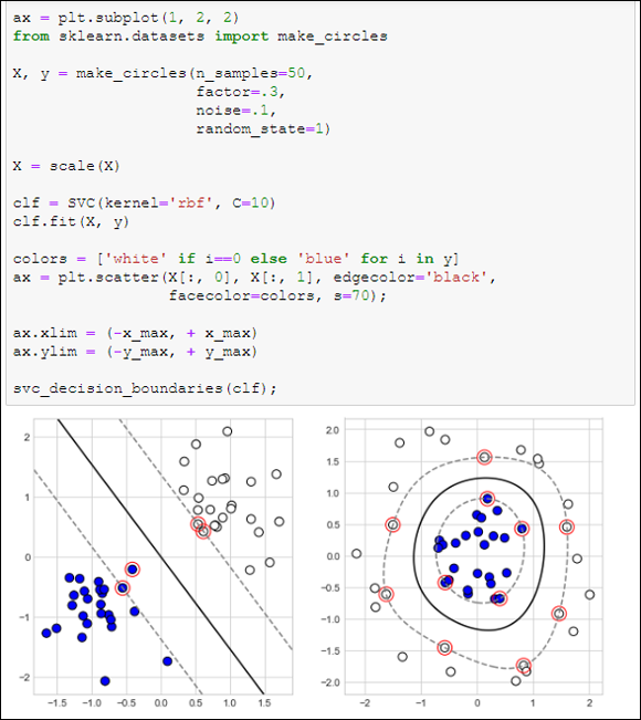
FIGURE 19-6: A viable SVM solution for the problem of the two groups and more.
The largest distance between the two groups is the margin. When the margin is large enough, you can be quite sure that it’ll keep working well, even when you have to classify previously unseen data. The margin is determined by the points that are present on the limit of the margin — the support vectors (the support vector machines algorithm takes its name from them).
You can see an SVM solution in the first pane in Figure 19-6. The figure shows the margin as a dashed line, the separator as the continuous line, and the support vectors as the circled data points.
Real-world problems don’t always provide neatly separable classes, as in this example. However, a well-tuned SVM can withstand some ambiguity (some misclassified points). An SVM algorithm with the right parameters can really do miracles.
When working with example data, it’s easier to look for neat solutions so that the data points can better explain how the algorithm works and you can grasp the core concepts. With real data, though, you need approximations that work. Therefore, you rarely see large and clear margins.
Apart from binary classifications on two dimensions, SVM can also work on complex data. You can consider the data as complex when you have more than two dimensions, or in situations that are similar to the layout depicted in the second pane in Figure 19-6, when separating the groups by a straight line isn’t possible.
 In the presence of many variables, SVM can use a complex separating plane (the hyperplane). SVM also works well when you can’t separate classes by a straight line or plane because it can explore nonlinear solutions in multidimensional space thanks to a computational technique called the kernel trick.
Fixing many new parameters
Although SVM is complex, it’s a great tool. After you find the most suitable SVM version for your problem, you have to apply it to your data and work a little to optimize some of the many parameters available and improve your results. Setting up a working SVM predictive model involves these general steps:
- Choose the SVM class you’ll use.
- Train your model with the data.
- Check your validation error and make it your baseline.
- Try different values for the SVM parameters.
- Check whether your validation error improves.
- Train your model again using the data with the best parameters.
To choose the right SVM class, you have to think about your problem. For example, you could choose a classification (guess a class) or regression (guess a number). When working with a classification, you must consider whether you need to classify just two groups (binary classification) or more than two (multiclass classification). Another important aspect to consider is the quantity of data you have to process. After taking notes of all your requirements on a list, a quick glance at Table 19-1 will help you to narrow your choices.
TABLE 19-1 The SVM Module of Learning Algorithms
Class |
Characteristic Usage |
Key Parameters |
sklearn.svm.SVC |
Binary and multiclass classification when the number of examples is less than 10,000 |
C, kernel, degree, gamma |
sklearn.svm.NuSVC |
Similar to SVC |
nu, kernel, degree, gamma |
sklearn.svm.LinearSVC |
Binary and multiclass classification when the number of examples is more than 10,000; sparse data |
Penalty, loss, C |
sklearn.svm.SVR |
Regression problems |
C, kernel, degree, gamma, epsilon |
sklearn.svm.NuSVR |
Similar to SVR |
Nu, C, kernel, degree, gamma |
sklearn.svm.OneClassSVM |
Outliers detection |
nu, kernel, degree, gamma |
The first step is to check the number of examples in your data. Having more than 10,000 examples could mean slow and cumbersome computations, but you can still use SVM to obtain acceptable performance for classification problems by using sklearn.svm.LinearSVC. When solving a regression problem, you may find that the LinearSVC isn’t fast enough, in which case you use a stochastic solution for SVM (as described in the sections that follow).
The Scikit-learn SVM module wraps two powerful libraries written in C, libsvm and liblinear. When fitting a model, there is a flow of data between Python and the two external libraries. A cache smooths the data exchange operations. However, if the cache is too small and you have too many data points, the cache becomes a bottleneck! If you have enough memory, it’s a good idea to set a cache size greater than the default 200MB (1000MB, if possible) using the SVM class’ cache_size parameter. Smaller numbers of examples require only that you decide between classification and regression.
In each case, you’ll have two alternative algorithms. For example, for classification, you may use sklearn.svm.SVC or sklearn.svm.NuSVC. The only difference with the Nu version is the parameters it takes and the use of a slightly different algorithm. In the end, it gets basically the same results, so you normally choose the non-Nu version.
After deciding on which algorithm to use, you find that you have a number of parameters from which to choose, and the C parameter is always among them. The C parameter indicates how much the algorithm has to adapt to training points. When C is small, the SVM adapts less to the points and tends to take an average direction, just using a few of the available points and variables. Larger C values tend to force the learning process to follow more of the available training points and to get involved with many variables.
The right C is usually a middle value, and you can find it after a bit of experimentation. If your C is too large, you risk overfitting, a situation in which your SVM adapts too much to your data and cannot properly handle new problems. If your C is too small, your prediction will be rougher and imprecise. You’ll experience a situation called underfitting — your model is too simple for the problem you want to solve.
After deciding the C value to use, the important block of parameters to fix is kernel, degree, and gamma. All three interconnect and their value depends on the kernel specification (for instance, the linear kernel doesn’t require degree or gamma, so you can use any value). The kernel specification determines whether your SVM model uses a line or a curve in order to guess the class or the point measure. Linear models are simpler and tend to guess well on new data, but sometimes underperform when variables in the data relate to each other in complex ways. Because you can’t know in advance whether a linear model works for your problem, it’s good practice to start with a linear kernel, fix its C value, and use that model and its performance as a baseline for testing nonlinear solutions afterward.
Classifying with SVC
It’s time to build the first SVM model. Because SVM initially performed so well with handwritten classification, starting with a similar problem is a great idea. Using this approach can give you an idea of how powerful this machine learning technique is. The example uses the digits dataset available from the module datasets in the Scikit-learn package. The digits dataset contains a series of 8-x-8-pixel images of handwritten numbers ranging from 0 to 9.
from sklearn import datasets
digits = datasets.load_digits()
X, y = digits.data, digits.target
After loading the datasets module, the load.digits function imports all the data, from which the example extracts the predictors (digits.data) as X and the predicted classes (digits.target) as y.
You can look at what’s inside this dataset using the matplotlib functions subplot (for creating an array of drawings arranged in two rows of five columns) and imshow (for plotting grayscale pixel values onto an 8-x-8 grid). The code arranges the information inside digits.images as a series of matrices, each one containing the pixel data of a number.
import matplotlib.pyplot as plt
%matplotlib inline
for k,img in enumerate(range(10)):
plt.subplot(2, 5, k+1)
plt.imshow(digits.images[img],
cmap='binary',
interpolation='none')
plt.show()
The code displays the first ten numbers as an example of the data used in the example. You can see the result in Figure 19-7.
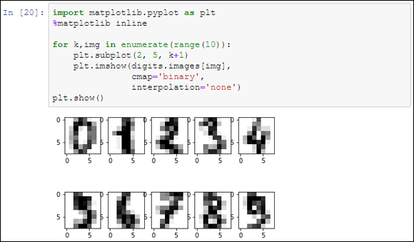
FIGURE 19-7: The first ten handwritten digits from the digits dataset.
By observing the data, you can also determine that SVM could guess a particular number by associating a probability with the values of specific pixels in the grid. A number 2 could turn on different pixels than a number 1, or maybe different groups of pixels. Data science involves testing many programming approaches and algorithms before reaching a solid result, but it helps to be imaginative and intuitive in order to determine which approach to try first. In fact, if you explore X, you discover that it’s made of exactly 64 variables, each one representing the grayscale value of a single pixel, and that you have plentiful examples — exactly 1,797 cases.
print(X[0])
The code returns a vector of the first example in the dataset:
[ 0. 0. 5. 13. 9. 1. 0. 0. 0. 0. 13. 15. 10. 15.
5. 0. 0. 3. 15. 2. 0. 11. 8. 0. 0. 4. 12. 0.
0. 8. 8. 0. 0. 5. 8. 0. 0. 9. 8. 0. 0. 4.
11. 0. 1. 12. 7. 0. 0. 2. 14. 5. 10. 12. 0. 0.
0. 0. 6. 13. 10. 0. 0. 0.]
If you reprint the same vector as an 8-x-8 matrix, you spot the image of a zero.
print(X[0].reshape(8, 8))
You interpret the zero values as the color white and the higher values as darker shades of gray:
[[ 0. 0. 5. 13. 9. 1. 0. 0.]
[ 0. 0. 13. 15. 10. 15. 5. 0.]
[ 0. 3. 15. 2. 0. 11. 8. 0.]
[ 0. 4. 12. 0. 0. 8. 8. 0.]
[ 0. 5. 8. 0. 0. 9. 8. 0.]
[ 0. 4. 11. 0. 1. 12. 7. 0.]
[ 0. 2. 14. 5. 10. 12. 0. 0.]
[ 0. 0. 6. 13. 10. 0. 0. 0.]]
At this point, you might wonder what to do about labels. You can try getting a count of the labels using the unique function in the NumPy package:
np.unique(y, return_counts=True)
The output associates the class label (the first number) with its frequency and is worth observing (it is the second row of output):
(array([0, 1, 2, 3, 4, 5, 6, 7, 8, 9]),
array([178, 182, 177, 183, 181, 182, 181, 179, 174, 180],
dtype=int64))
All the class labels present about the same number of examples. That means that your classes are balanced and that the SVM won’t be led to think that one class is more probable than any of the others. If one or more of the classes had a significantly different number of cases, you’d face an unbalanced class problem. An unbalanced class scenario requires you to perform an evaluation:
- Keep the unbalanced class and get predictions biased toward the most frequent classes
- Establish equality among the classes using weights, which means allowing some observations to count more
- Use selection to cut some cases from the classes that have too many cases
An imbalanced class problem requires you to set some additional parameters. sklearn.svm.SVC has both a class_weight parameter and a sample_weight keyword in the fit method. The most straightforward and easiest way to solve the problem is to set class_weight=’auto’ when defining your SVC and let the algorithm fix everything by itself.
Now you’re ready to test the SVC with the linear kernel. However, don’t forget to split your data into training and test sets, or you won’t be able to judge the effectiveness of the modeling work. Always use a separate data fraction for performance evaluation or the results will look good at the start but turn worse when adding fresh data.
from sklearn.model_selection import train_test_split
from sklearn.model_selection import cross_val_score
from sklearn.preprocessing import MinMaxScaler
X_tr, X_t, y_tr, y_t = train_test_split(X, y,
test_size=0.3,
random_state=0)
The train_test_split function splits X and y into training and test sets, using the test_size parameter value of 0.3 as a reference for the split ratio.
scaling = MinMaxScaler(feature_range=(-1, 1)).fit(X_tr)
X_tr = scaling.transform(X_tr)
X_t = scaling.transform(X_t)
As a best practice, after splitting the data into training and test parts, you scale the numeric values, first by getting scaling parameters from the training data and then by applying a transformation on both training and test sets.
Another important action to take before feeding the data into an SVM is scaling. Scaling transforms all the values to the range between –1 to 1 (or from 0 to 1, if you prefer). Scaling transformation avoids the problem of having some variables influence the algorithm (they may trick it into thinking they are important because they have big values) and it makes the computations exact, smooth, and fast.
The following code fits the training data to an SVC class with a linear kernel. It also cross-validates and tests the results in terms of accuracy (the percentage of numbers correctly guessed).
from sklearn.svm import SVC
svc = SVC(kernel='linear',
class_weight='balanced')
The code instructs the SVC to use the linear kernel and to reweight the classes automatically. Reweighting the classes ensures that they remain equally sized after the dataset is split into training and test sets.
cv = cross_val_score(svc, X_tr, y_tr, cv=10)
test_score = svc.fit(X_tr, y_tr).score(X_t, y_t)
The code then assigns two new variables. Cross-validation performance is recorded by the cross_val_score function, which returns a list with all ten scores after a ten-fold cross-validation (cv=10). The code obtains a test result by using two methods in sequence on the learning algorithm — fit, that fits the model, and score, which evaluates the result on the test set using mean accuracy (mean percentage of correct results among the classes to predict).
print('CV accuracy score: %0.3f' % np.mean(cv))
print('Test accuracy score: %0.3f' % (test_score))
Finally, the code prints the two variables and evaluates the result. The result is quite good: 97.4 percent correct predictions on the test set:
CV accuracy score: 0.983
Test accuracy score: 0.976
You might wonder what would happen if you optimize the principal parameter C instead of using the default value of 1.0. The following script provides you with an answer, using gridsearch to look for an optimal value for the C parameter:
from sklearn.model_selection import GridSearchCV
svc = SVC(class_weight='balanced', random_state=1)
search_space = {'C': np.logspace(-3, 3, 7)}
gridsearch = GridSearchCV(svc,
param_grid=search_space,
scoring='accuracy',
refit=True, cv=10)
gridsearch.fit(X_tr,y_tr)
Using GridSearchCV is a little more complex, but it allows you to check many models in sequence. First, you must define a search space variable using a Python dictionary that contains the exploration schedule of the procedure. To define a search space, you create a dictionary (or, if there is more than one dictionary, a dictionary list) for each tested group of parameters. Inside the dictionary, you place the name of the parameters as keys and associate them with a list (or a function generating a list, as in this case) containing the values to test.
The NumPy logspace function creates a list of seven C values, ranging from 10^–3 to 10^3. This is a computationally expensive number of values to test, but it’s also comprehensive, and you can always be safe when you test C and the other SVM parameters using such a range.
You then initialize GridSearchCV, defining the learning algorithm, search space, scoring function, and number of cross-validation folds. The next step is to instruct the procedure, after finding the best solution, to fit the best combination of parameters, so that you can have a ready-to-use predictive model:
cv = gridsearch.best_score_
test_score = gridsearch.score(X_t, y_t)
best_c = gridsearch.best_params_['C']
In fact, gridsearch now contains a lot of information about the best score (and best parameters, plus a complete analysis of all the evaluated combinations) and methods, such as score, which are typical of fitted predictive models in Scikit-learn.
print('CV accuracy score: %0.3f' % cv)
print('Test accuracy score: %0.3f' % test_score)
print('Best C parameter: %0.1f' % best_c)
Here, the code extracts cross-validation and test scores, and outputs the C value related to these best scores:
CV accuracy score: 0.989
Test accuracy score: 0.987
Best C parameter: 10.0
The last step prints the results and shows that using a C=100 increases performance compared to before, both on the cross-validation and the test set.
Going nonlinear is easy
Having defined a simple linear model as a benchmark for the handwritten digit project, you can now test a more complex hypothesis, and SVM offers a range of nonlinear kernels:
- Polynomial (poly)
- Radial Basis Function (rbf)
- Sigmoid (sigmoid)
- Advanced custom kernels
Even though so many choices exist, you rarely use something different from the radial basis function kernel (rbf for short) because it’s faster than other kernels and can approximate almost any nonlinear function.
Here’s a basic, practical explanation about how rbf works: It separates the data into many clusters, so it’s easy to associate a response to each cluster.
The rbf kernel requires that you set the degree and gamma parameters besides setting C. They’re both easy to set (and a good grid search will always find the right value).
The degree parameter has values that begin at 2. It determinates the complexity of the nonlinear function used to separate the points. As a practical suggestion, don’t worry too much about degree — test values of 2, 3, and 4 on a grid search. If you notice that the best result has a degree of 4, try shifting the grid range upward and test 3, 4, and 5. Continue proceeding upward as needed, but using a value greater than 5 is rare.
The gamma parameter’s role in the algorithm is similar to C (it provides a trade-off between overfit and underfit). It’s exclusive of the rbf kernel. High gamma values induce the algorithm to create nonlinear functions that have irregular shapes because they tend to fit the data more closely. Lower values create more regular, spherical functions, ignoring most of the irregularities present in the data.
Now that you know the details of the nonlinear approach, it’s time to try rbf on the previous example. Be warned that, given the high number of combinations tested, the computations may take some time to complete, depending on the characteristics of your computer.
from sklearn.model_selection import GridSearchCV
svc = SVC(class_weight='balanced', random_state=101)
search_space = [{'kernel': ['linear'],
'C': np.logspace(-3, 3, 7)},
{'kernel': ['rbf'],
'degree':[2, 3, 4],
'C':np.logspace(-3, 3, 7),
'gamma': np.logspace(-3, 2, 6)}]
gridsearch = GridSearchCV(svc,
param_grid=search_space,
scoring='accuracy',
refit=True, cv=10,
n_jobs=-1)
gridsearch.fit(X_tr, y_tr)
cv = gridsearch.best_score_
test_score = gridsearch.score(X_t, y_t)
print('CV accuracy score: %0.3f' % cv)
print('Test accuracy score: %0.3f' % test_score)
print(’Best parameters: %s’ % gridsearch.best_params_)Notice that the only difference in this script is that the search space is more sophisticated. By using a list, you enclose two dictionaries — one containing the parameters to test for the linear kernel and another for the rbf kernel. In this way, you can compare the performance of the two approaches at the same time. The code will take quite a while to run. Afterwards, it will report to you:
CV accuracy score: 0.990
Test accuracy score: 0.993
Best parameters: {'C': 1.0, 'degree': 2,
'gamma': 0.1, 'kernel': 'rbf'}
The results confirm that rbf performs better. However, it’s a small margin of victory over the linear models, gained at the expense of more complexity and computational time. In such cases, having more data available could help in determining the better model with greater confidence. Unfortunately, getting more data may be expensive in terms of money and time. When faced with the absence of a clear winning model, the best suggestion is to decide in favor of the simpler model. In this case, the linear kernel is much simpler than rbf.
Performing regression with SVR
Up to now, you have dealt only with classification, but SVM can also handle regression problems. Having seen how a classification works, you don’t need to know much more than that the SVM regression class is SVR and there is a new parameter to fix, epsilon. Everything else previous sections discussed for classification works precisely the same with regression.
This example uses a different dataset, a regression dataset. The Boston house price dataset, taken from the StatLib library maintained at Carnegie Mellon University, appears in many machine learning and statistical papers that address regression problems. It has 506 cases and 13 numeric variables (one of which is a 1/0 binary variable).
from sklearn.model_selection import train_test_split
from sklearn.model_selection import cross_val_score
from sklearn.model_selection import GridSearchCV
from sklearn.preprocessing import MinMaxScaler
from sklearn.svm import SVR
from sklearn import datasets
boston = datasets.load_boston()
X,y = boston.data, boston.target
X_tr, X_t, y_tr, y_t = train_test_split(X, y,
test_size=0.3,
random_state=0)
scaling = MinMaxScaler(feature_range=(-1, 1)).fit(X_tr)
X_tr = scaling.transform(X_tr)
X_t = scaling.transform(X_t)
The target is the median value of houses occupied by an owner, and you’ll try to guess it using SVR (epsilon-Support Vector Regression). In addition to C, kernel, degree, and gamma, SVR also has epsilon. Epsilon is a measure of how much error the algorithm considers acceptable. A high epsilon implies fewer support points, while a lower epsilon requires a larger number of support points. In other words, epsilon provides another way to trade-off underfit against overfit.
As a search space for this parameter, experience tells you that the sequence [0, 0.01, 0.1, 0.5, 1, 2, 4] works quite fine. Starting from a minimum value of 0 (when the algorithm doesn’t accept any error) and reaching a maximum of 4, you should enlarge the search space only if you notice that higher epsilon values bring better performance.
Having included epsilon in the search space and assigning SVR as a learning algorithm, you can complete the script. Be warned that, given the high number of combinations evaluated, the computations may take quite some time, depending on the characteristics of your computer.
svr = SVR()
search_space = [{'kernel': ['linear'],
'C': np.logspace(-3, 2, 6),
'epsilon': [0, 0.01, 0.1, 0.5, 1, 2, 4]},
{'kernel': ['rbf'],
'degree':[2, 3],
'C':np.logspace(-3, 3, 7),
'gamma': np.logspace(-3, 2, 6),
'epsilon': [0, 0.01, 0.1, 0.5, 1, 2, 4]}]
gridsearch = GridSearchCV(svr,
param_grid=search_space,
refit=True,
scoring= 'r2',
cv=10, n_jobs=-1)
gridsearch.fit(X_tr, y_tr)
cv = gridsearch.best_score_
test_score = gridsearch.score(X_t, y_t)
print('CV R2 score: %0.3f' % cv)
print('Test R2 score: %0.3f' % test_score)
print('Best parameters: %s' % gridsearch.best_params_)
The grid search may take a while on your computer. Even though the example uses all the computational power in your system (n_jobs=-1), the computer has to test quite a few combinations; for each kernel, you can figure out how many models it has to compute by multiplying the number of values it has to test for each parameter. For instance for the rbf kernel, it has two values for degree, seven for C, six for gamma, and seven for epsilon, which equates to 2 * 7 * 6 * 7 = 588 models, each one replicated 10 times (because cv=10). That is 5,880 models tested just for the rbf kernel (the code also tests the linear model, which requires 420 tests). Finally, you should get these results:
CV R2 score: 0.868
Test R2 score: 0.834
Best parameters: {'C': 1000.0, 'degree': 2, 'epsilon': 2,
'gamma': 0.1, 'kernel': 'rbf'}
Note that on the error measure, as a regression, the error is calculated using R squared, a measure in the range from 0 to 1 that indicates the model’s performance (with 1 being the best possible result to achieve).
Creating a stochastic solution with SVM
Now that you’re at the end of the overview of the family of SVM machine learning algorithms, you should see that they’re a fantastic tool for a data scientist. Of course, even the best solutions have problems. For example, you might think that the SVM has too many parameters in the SVM. Certainly, the parameters are a nuisance, especially when you have to test so many combinations of them, which can take a lot of CPU time. However, the key problem is the time necessary for training the SVM. You may have noticed that the examples use small datasets with a limited number of variables, and performing some extensive grid searches still takes a lot of time. Real-world datasets are much bigger. Sometimes it may seem to take forever to train and optimize your SVM on your computer.
A possible solution when you have too many cases (a suggested limit is 10,000 examples) is found inside the same SVM module, the LinearSVC class. This algorithm works only with the linear kernel and its focus is to classify (sorry, no regression) large numbers of examples and variables at a higher speed than the standard SVC. Such characteristics make the LinearSVC a good candidate for textual-based classification. LinearSVC has fewer and slightly different parameters to fix than the usual SVM (it’s similar to a regression class):
C: The penalty parameter. Small values imply more regularization (simpler models with attenuated or set to zero coefficients).loss: A value ofl1(just as in SVM) orl2(errors weight more, so it strives harder to fit misclassified examples).penalty: A value ofl2(attenuation of less important parameters) orl1(unimportant parameters are set to zero).dual: A value oftrueorfalse. It refers to the type of optimization problem solved and, though it won’t change the obtained scoring much, setting the parameter tofalseresults in faster computations than when it is set totrue.
The loss, penalty, and dual parameters are also bound by reciprocal constraints, so please refer to Table 19-2 to plan which combination to use in advance.
TABLE 19-2 The Loss, Penalty, and Dual Constraints
Penalty |
Loss |
Dual |
l1 |
l2 |
False |
l2 |
l1 |
True |
l2 |
l2 |
True; False |
The algorithm doesn’t support the combination of penalty=’l1’ and loss=’l1’. However, the combination of penalty=’l2’ and loss=’l1’ perfectly replicates the SVC optimization approach.
As mentioned previously, LinearSVC is quite fast, and a speed test against SVC demonstrates the level of improvement to expect in choosing this algorithm.
from sklearn.datasets import make_classification
from sklearn.model_selection import train_test_split
import numpy as np
X,y = make_classification(n_samples=10**4,
n_features=15,
n_informative=10,
random_state=101)
X_tr, X_t, y_tr, y_t = train_test_split(X, y,
test_size=0.3,
random_state=1)
from sklearn.svm import SVC, LinearSVC
svc = SVC(kernel='linear', random_state=1)
linear = LinearSVC(loss='hinge', random_state=1)
svc.fit(X_tr, y_tr)
linear.fit(X_tr, y_tr)
svc_score = svc.score(X_t, y_t)
libsvc_score = linear.score(X_t, y_t)
print('SVC test accuracy: %0.3f' % svc_score)
print('LinearSVC test accuracy: %0.3f' % libsvc_score)
The results are quite similar to SVC:
SVC test accuracy: 0.803
LinearSVC test accuracy: 0.804
After you create an artificial dataset using make_classfication, the code obtains confirmation of how the two algorithms arrive at almost identical results. At this point, the code tests the speed of the two solutions on the synthetic dataset in order to understand how they scale to use more data.
import timeit
X,y = make_classification(n_samples=10**4,
n_features=15,
n_informative=10,
random_state=101)
t_svc = timeit.timeit('svc.fit(X, y)',
'from __main__ import svc, X, y',
number=1)
t_libsvc = timeit.timeit('linear.fit(X, y)',
'from __main__ import linear, X, y',
number=1)
print('best avg secs for SVC: %0.1f' % np.mean(t_svc))
print('best avg secs for LinearSVC: %0.1f' % np.mean(t_libsvc))
The example system shows the following result (the output of your system may differ):
avg secs for SVC, best of 3: 16.6
avg secs for LinearSVC, best of 3: 0.4
Clearly, given the same data quantity, LinearSVC is much faster than SVC. You can calculate its performance ratio as 16.6 / 0.4 = 41.5 times faster than SVC. However, it’s important to understand what happens when you increase the size of the sample. For example, here’s what happens when you triple the size:
avg secs for SVC, best of 3: 162.6
avg secs for LinearSVC, best of 3: 2.6
The point here is that the time required for SVC grows faster (9.8 times) than that required by LinearSVC (6.5 times). This is because SVC requires proportionally more time to process the data provided and the time will grow even more as the sample size increases. Here are the results when you have five times more data, highlighting even more differences:
avg secs for SVC, best of 3: 539.1
avg secs for LinearSVC, best of 3: 4.5
Using SVC with large amounts of data soon becomes unfeasible; LinearSVC should be your choice if you need to work with large data amounts. Yet, even if LinearSVC is quite fast at performing tasks, you may need to classify or regress millions of examples. You need to know whether LinearSVC is still a better choice. You previously saw how the SGD class, using SGDClassifier and SGDRegressor, helps you implement an SVM-type algorithm in situations with millions of data rows without investing too much computational power. All you have to do is to set their loss to ’hinge’ for SGDClassifier and to ’epsilon_insensitive’ for SGDRegressor (in which case, you have to tune the epsilon parameter).
Another performance and speed test makes the advantages and limitations of using LinearSVC or SGDClassifier clear:
from sklearn.datasets import make_classification
from sklearn.model_selection import train_test_split
from sklearn.model_selection import cross_val_score
from sklearn.svm import LinearSVC
import timeit
from sklearn.linear_model import SGDClassifier
X, y = make_classification(n_samples=10**5,
n_features=15,
n_informative=10,
random_state=101)
X_tr, X_t, y_tr, y_t = train_test_split(X, y,
test_size=0.3,
random_state=1)
The sample now is quite big — 100,000 cases. If you have enough memory and a lot of time, you may even want to increase the number of trained cases or the number of features and more extensively test how the two algorithms scale with even bigger data.
linear = LinearSVC(penalty='l2',
loss='hinge',
dual=True,
random_state=1)
linear.fit(X_tr, y_tr)
score = linear.score(X_t, y_t)
t = timeit.timeit("linear.fit(X_tr, y_tr)",
"from __main__ import linear, X_tr, y_tr",
number=1)
print('LinearSVC test accuracy: %0.3f' % score)
print('Avg time for LinearSVC: %0.1f secs' % np.mean(t))
On the test computer, LinearSVC completed its computations on all the rows in about seven seconds:
LinearSVC test accuracy: 0.796
Avg time for LinearSVC: 7.4 secs
The following code tests SGDClassifier using the same procedure:
sgd = SGDClassifier(loss='hinge',
max_iter=100,
shuffle=True,
random_state=101)
sgd.fit(X_tr, y_tr)
score = sgd.score(X_t, y_t)
t = timeit.timeit("sgd.fit(X_tr, y_tr)",
"from __main__ import sgd, X_tr, y_tr",
number=1)
print('SGDClassifier test accuracy: %0.3f' % score)
print('Avg time SGDClassifier: %0.1f secs' % np.mean(t))
SGDClassifier instead took about a second and a half for processing the same data and obtaining a comparable, score:
SGDClassifier test accuracy: 0.796
Avg time SGDClassifier: 1.5 secs
Increasing the n_iter parameter can improve the performance, but it proportionally increases the computation time. Increasing the number of iterations up to a certain value (that you have to find out by test) increases the performance. However, after that value, performance starts to decrease because of overfitting.
Playing with Neural Networks
Starting with the idea of reverse-engineering how a brain processes signals, researchers based neural networks on biological analogies and their components, using brain terms such as neurons and axons as names. However, you’ll discover that neural networks resemble nothing more than a sophisticated kind of linear regression because they are a summation of coefficients multiplied by numeric inputs. You also find that neurons are just where such summations happen.
Even if neural networks don’t mimic a brain (they’re arithmetic), these algorithms are extraordinarily effective against complex problems such as image and sound recognition, or machine language translation. They also execute quickly when predicting, if you use the right hardware. Well-devised neural networks use the name deep learning and are behind powerful tools like Siri and other digital assistants, along with more astonishing machine learning applications as well.
Running deep learning requires special hardware (a computer with a GPU) and installing special frameworks such as Tensorflow (https://www.tensorflow.org/), MXNet (https://mxnet.apache.org/), Pytorch (https://pytorch.org/) or Chainer (https://chainer.org/). This book doesn’t delve into complex neural networks but does explore a simpler implementation offered by Scikit-learn instead, which allows you to create neural network quickly and compare them to other machine learning algorithms.
Understanding neural networks
The core neural network algorithm is the neuron (also called a unit). Many neurons arranged in an interconnected structure make up the layers of a neural network, with each neuron linking to the inputs and outputs of other neurons. Thus, a neuron can input features from examples or from the results of other neurons, depending on its location in the neural network.
Contrary to other algorithms, which have a fixed pipeline that determines how algorithms receive and process data, neural networks require you to decide how information flows by fixing the number of units (the neurons) and their distribution in layers. For this reason, setting up neural networks is more an art than a science; you learn from experience how to arrange neurons into layers and obtain the best predictions. In a more detailed view, neurons in a neural network take many weighted values as inputs, sum them, and provide the summation as the result.
A neural network can process only numeric, continuous information; it can’t process qualitative variables (for example, labels indicating a quality such as red, blue, or green in an image). You can process qualitative variables by transforming them into a continuous numeric value, such as a series of binary values
Neurons also provide a more sophisticated transformation of the summation. In observing nature, scientists noticed that neurons receive signals but don’t always release a signal of their own. It depends on the amount of signal received. When a neuron in a brain acquires enough stimuli, it fires an answer; otherwise, it remains silent. In a similar fashion, neurons in a neural network, after receiving weighted values, sum them and use an activation function to evaluate the result, which transforms it in a nonlinear way. For instance, the activation function can release a zero value unless the input achieves a certain threshold, or it can dampen or enhance a value by nonlinearly rescaling it, thus transmitting a rescaled signal.
Each neuron in the network receives inputs from the previous layers (when starting, it connects directly with data), weights them, sums them all, and transforms the result using the activation function. After activating, the computed output becomes the input for other neurons or the prediction of the network. Consequently, given a neural network made of a certain number of neurons and layers, what makes this structure efficient in its predictions is the weights used by each neuron for its inputs. Such weights aren’t different from the coefficients of a linear regression, and the network learns their value by repeated passes (iterations or epochs) over the examples of the dataset.
Classifying and regressing with neurons
Scikit-learn offers two functions for neural networks:
MLPClassifier: Implements a multilayer perceptron (MLP) for classification. Its outputs (one or many, depending on how many classes you have to predict) are intended as probabilities of the example being of a certain class.MLPRegressor: Implements MLP for regression problems. All its outputs (because it can predict multiple target values at one time) are intended as estimates of the measures to predict.
Because both functions have the exact same parameters, the example delves into a single example for classification, using the handwritten digits as an example of multiclass classification using a MLP. The example starts by importing the necessary packages, loading the dataset into memory, and splitting it into a training and a test set (as the chapter has done when demonstrating support vector machines):
from sklearn.model_selection import train_test_split
from sklearn.model_selection import cross_val_score
from sklearn.preprocessing import MinMaxScaler
from sklearn import datasets
from sklearn.neural_network import MLPClassifier
digits = datasets.load_digits()
X, y = digits.data, digits.target
X_tr, X_t, y_tr, y_t = train_test_split(X, y,
test_size=0.3,
random_state=0)
Preprocessing the data to feed to the neural network is an important aspect because the operations that neural networks perform under the hood are sensitive to the scale and distribution of data. Consequently, it’s good practice to normalize the data by putting its mean to zero and its variance to one, or to rescale it by fixing the minimum and maximum between –1 and +1 or 0 and +1. Experimentation shows which transformation works better for your data, though most people find that rescaling between –1 and +1 works better. This example rescales all the values between –1 and +1.
scaling = MinMaxScaler(feature_range=(-1, 1)).fit(X_tr)
X_tr = scaling.transform(X_tr)
X_t = scaling.transform(X_t)
As discussed earlier, it’s good practice to define the preprocessing transformations on the training data alone and then apply the learned procedure to the test data. Only in this way can you correctly test how your model works with different data.
To define MLP, you must consider that there are quite a few parameters and if you don’t tune them correctly, the results may be disappointing. (MLP is not an algorithm that works out of the box.) For an MLP to work properly, you should first define the architecture of the neurons, setting how many to use for each layer and how many layers to create. (You state the number of neurons for each layer in the hidden_layer_sizes parameter.) Then you have to determine the right solver among:
- L-BFGS: Use for small datasets.
- Adam: Use for large datasets.
- SGD: Excels at most problems if you correctly set some special parameters. L-BFGS works for small datasets, Adam for large ones, and SDG can excel at most problems if you set its parameters correctly. SGD’s parameters are the learning rate, which can reflect learning speed, and momentum (or Nesterov’s momentum), a value that helps the neural network to avoid less useful solutions. When specifying the learning rate, you have to define its starting value (
learning_rate_init, which is usually around 0.001, but it can be even less) and how the speed changes during training (thelearning_rateparameter, which can be’constant’,’invscaling’, or’adaptive’).
Given the complexity of setting the parameters for an SGD solver, you can determine how they work on your data only by testing them in a hyperparameter optimization. Most people prefer to start with an L-BFGS or Adam solver.
Another critical hyperparameter is max_iter, the number of iterations, which can lead to completely different results if you set it too low or too high. The default is 200 iterations, but it’s always better, after having fixed the other parameters, to try to increase or decrease its number. Finally, shuffling the data (shuffle=True) and setting a random_state for reproducibility of results are also important. The example code sets 512 nodes on a single layer, relies on the Adam solver, and uses the standard number of iterations (200):
nn = MLPClassifier(hidden_layer_sizes=(512, ),
activation='relu',
solver='adam',
shuffle=True,
tol=1e-4,
random_state=1)
cv = cross_val_score(nn, X_tr, y_tr, cv=10)
test_score = nn.fit(X_tr, y_tr).score(X_t, y_t)
print('CV accuracy score: %0.3f' % np.mean(cv))
print('Test accuracy score: %0.3f' % (test_score))
Using this code, the example successfully classifies handwritten digits by running an MLP whose CV and test score are
CV accuracy score: 0.978
Test accuracy score: 0.981
The results obtained are a little better than SVC’s, yet the increase involves tuning quite a few parameters correctly as well. When using nonlinear algorithms, you can’t expect any no-brainer approach, apart from a few decision-tree based solutions, which is the topic of the next chapter.