
Chapter 15
Clustering
IN THIS CHAPTER
![]() Exploring the potentialities of unsupervised clustering
Exploring the potentialities of unsupervised clustering
![]() Making K-means work with small and big data
Making K-means work with small and big data
![]() Trying DBScan as an alternative option
Trying DBScan as an alternative option
One of the basic abilities that humans have exercised since primitive times is to divide the known world into separate classes where individual objects share common features deemed important by the classifier. Starting with primitive cave dwellers classifying the natural world they lived in, distinguishing plants and animals useful or dangerous for their survival, we arrive at modern times in which marketing departments classify consumers into target segments and then act with proper marketing plans.
Classifying is crucial to our process of building new knowledge because, by gathering similar objects, we can:
- Mention all the items in a class by the same denomination
- Summarize relevant features by an exemplificative class type
- Associate particular actions or recall specific knowledge automatically
Dealing with big data streams today requires the same classificatory ability, but on a different scale. To spot unknown groups of signals present in the data, we need specialized algorithms that are both able to learn how to assign examples to certain given classes (the supervised approach) and to spot new interesting classes that we weren’t aware of (unsupervised learning).
Even though your main routine as a data scientist will be to put into practice your predictive skills, you’ll also have to provide useful insight into possible novel information present in your data. For example, you’ll often need to locate new features in order to strengthen the predictive power of your models, find an easy way to make complex comparisons inside the data, and discover communities in social networks.
A data-driven approach to classification, called clustering, will prove to be of great help in achieving success for your data project when you need to provide new insights from scratch and you lack labeled data or you want to create new labels for it.
Clustering techniques are a set of unsupervised classification methods that can create meaningful classes by directly processing your data, without any previous knowledge or hypothesis about the groups that may be present. If all supervised algorithms need labeled examples (class labels), unsupervised ones can figure out by themselves what the most appropriate labels could be.
 Clustering can help you to summarize huge quantities of data. It is an effective technique for presenting data to a nontechnical audience and for feeding a supervised algorithm with group variables, thus providing them with concentrated, significant information.
There are a few kinds of clustering techniques. You can distinguish between them using the guidelines in the following list:
- Assigning every example to a unique group (partitioning) or to multiple ones (fuzzy clustering)
- Determining the heuristic — that is, the rule of thumb — that they use to figure out whether an example is part of a group
- Specifying how they quantify the difference between observations, that is, the so-called distance measure
Most of the time you use partition-clustering techniques (a data point can be part of only one group, so the groups don’t overlap; their membership is distinct) and among partitioning methods, you use K-means the most. In addition, other useful methods are mentioned in this chapter, which are based on agglomerative methods and on data density.
Agglomerative methods set data into clusters based on a distance measure. Data density approaches take advantage of the idea that groups are very dense and continuous, so if you notice a decrease in density when exploring a part of a group of points, it could mean that you arrived at one of its borders.
Because you normally don’t know what you’re looking for, different methods can provide you with different solutions and points of view on the data. The secret of a successful clustering is to try as many of the recipes as possible, compare the results, and try to find a reason why you can consider certain observations as a group in respect to others.
 You don’t have to type the source code for this chapter manually. In fact, it’s a lot easier if you use the downloadable source (see the Introduction for download instructions). The source code for this chapter appears in the
 P4DS4D2_15_Clustering.ipynb source code file.
Clustering with K-means
K-means is an iterative algorithm that has become very popular in machine learning because of its simplicity, speed, and scalability to a large number of data points. The K-means algorithm relies on the idea that there are a specific number of data groups, called clusters. Each data group is scattered around a central point with which they share some key characteristics.
You can actually imagine the central point of a cluster, called a centroid, as a sun. The data points distribute around the centroid like planets. As star systems are separated by the void of space, clusters are also expected to clearly separate from each other, so, as groups of points they are both internally homogeneous and different from each other.
The K-means algorithm expects to find clusters in your data. Therefore, it will find them even when none exist. It’s important to check inside the groups to determine whether the group is a true gold nugget.
Given such assumptions, all you have to do is to specify the number of groups you expect (you can use a guess or try a number of possible desirable solutions), and the K-means algorithm will look for them, using a heuristic in order to recover the position of the central points.
The cluster centroids should be evident by their different characteristics and positions from each other. Even if you start by randomly guessing where they could be, in the end, after a few corrections, you always find them by using the many data points that gravitate around them.
Understanding centroid-based algorithms
The procedure for finding the centroids is straightforward:
Guess a K number of clusters.
K centroids are picked randomly from your data points or chosen so that they are placed in your data in very distant positions from each other. All the other points are assigned to their nearest centroid based on the Euclidean distance.
- Form the initial clusters.
Reiterate the clusters until you notice that your solution doesn’t change anymore.
You recalculate the centroids as an average of all the points present in the group. All the data points are reassigned to the groups based on the distance from the new centroids.
The iterative process of assigning cases to the most plausible centroid and then averaging the assigned ones to find a new centroid will slowly shift the centroid position toward the areas where most data points gravitate. The result is that you end up with the true centroid position.
The procedure has only two weak points that you need to consider. First, you choose the initial centroids randomly, which means that you could start from a bad starting point. As a result, the iterative process will stop at some unlikely solution — for example, having a centroid in the middle of two groups. To ensure that your solution is the most probable, you have to try the algorithm a few times and track the results. The more often you try, the more likely you are to confirm the right solution. The Python Scikit-learn implementation of K-means will do that for you, so you just have to decide how many times you intend to try. (The trade-off is that more iterations produce better results, but each iteration consumes valuable time.)
The second weak point is due to the distance that K-means uses, the Euclidean distance, which is the distance between two points on a plane (a concept that you likely studied at school). In a K-means application, each data point is a vector of features, so when comparing the distance of two points, you do the following:
- Create a list containing the differences of the elements in the two vectors.
- Square all the elements of the difference vector.
- Calculate the square root of the summed elements.
You can try a simple example in Python. Pretend that you have two points, A and B, and they have three numeric features. If A and B are the data representation of two persons, their distinguishing features could be measured in height (cm), weight (kg), and age (years), as shown in the following code:
import numpy as np
A = np.array([165, 55, 70])
B = np.array([185, 60, 30])
The following example shows how to calculate the differences between the three elements, square all the resulting elements, and determine the square root of the summed squared values:
D = (A - B)
D = D**2
D = np.sqrt(np.sum(D))
print(D)
45.0
In the end, the Euclidean distance is really just a big sum. When the variables making up the difference vector are significantly different in scale from each other (in this example, the height could have been expressed in meters), you end up with a distance dominated by the elements with the largest scale. It is very important to rescale the variables so that they use a similar scale before applying the K-means algorithm. You can use a fixed range or a statistical normalization with zero mean and unit variance to achieve this goal.
Another problem that may arise is due to correlation between variables, causing redundancy of information. If two variables are highly correlated, that means that a part of their information content is repeated. Replication implies counting the same information more than once in the summation used to calculate the distance. If you’re not aware of the correlation issue, some variables will dominate your distance measure calculation — a situation that may lead to not finding the useful clusters that you want. The solution is to remove the correlation thanks to a dimensionality reduction algorithm such as Principle Component Analysis (PCA). It is up to you to remember to evaluate scale and correlation before employing K-means and other clustering techniques using the Euclidean distance measure.
Creating an example with image data
An example with image data demonstrates how to apply the tool and how to get insight from clusters. An ideal example is clustering the handwritten digits dataset provided by the Scikit-learn package. Hand-written numbers are naturally different from each other — they possess variability in that there are several ways to write certain numbers. Of course, we all have different writing styles, so it is natural that each person’s numbers differ slightly. The following code shows how to import the image data.
from sklearn.datasets import load_digits
digits = load_digits()
X = digits.data
ground_truth = digits.target
The example begins by importing the digits dataset from Scikit-learn and assigning the data to a variable. It then stores the labels in another variable for later verification. The next step is to process the data using a PCA.
from sklearn.decomposition import PCA
from sklearn.preprocessing import scale
pca = PCA(n_components=30)
Cx = pca.fit_transform(scale(X))
print('Explained variance %0.3f'
% sum(pca.explained_variance_ratio_))
Explained variance 0.893
By applying a PCA on scaled data, the code addresses the problems of scale and correlation. Even though PCA can recreate the same number of variables as in the input data, the example code drops a few using the n_components parameter. The decision to use 30 components, as compared to the original 64 variables, allows the example to retain most of the original information (about 90 percent of the original variation in data) and simplify the dataset by removing correlation and reducing redundant variables and their noise.
The remainder of the chapter uses the Cx dataset. If you need to run single, isolated code examples from the chapter, you need to run the code presented earlier in this paragraph first.
In this example, the PCA-transformed data appears in the Cx variable. After importing the KMeans class, the code defines its main parameters:
n_clustersis the K number of centroids to find.n_initis the number of times to try the K-means with different starting centroids. The code needs to test the procedure a sufficient number of times, such as 10, as shown here.from sklearn.cluster import KMeansclustering = KMeans(n_clusters=10,n_init=10, random_state=1)clustering.fit(Cx)
After creating the parameters, the clustering class is ready for use. You can apply the fit() method to the Cx dataset, which produces a scaled and dimensionally reduced dataset.
Looking for optimal solutions
As mentioned in the previous section, the example is clustering ten different numbers. It’s time to start checking the solution with K = 10 first. The following code compares the previous clustering result to the ground truth — the true labels — in order to determine whether there is any correspondence.
import numpy as np
import pandas as pd
ms = np.column_stack((ground_truth,clustering.labels_))
df = pd.DataFrame(ms,
columns = ['Ground truth','Clusters'])
pd.crosstab(df['Ground truth'], df['Clusters'],
margins=True)
Converting the solution, given by the labels variable internal to the clustering class, into a pandas DataFrame allows it to apply a cross-tabulation and compare the original labels with the labels derived from clustering. You can observe the results in Figure 15-1. Because rows represent ground truth, you can look for numbers whose majority of observations are split among different clusters. These observations are the handwritten examples that are more difficult to figure out by K-means.

FIGURE 15-1: Cross-tabulation of ground truth and K-means clusters.
Notice how numbers such as six or zero are concentrated into a single major cluster, whereas others, such as three, nine and many examples from five and eight, tend to gather into the same group, cluster 1. Cluster 9 consists of a single number four (an example that’s so different from all others that that it has its own cluster). From such a discovery, you can deduce that certain handwritten numbers are easy to guess, while others aren’t.
Cross-tabulation has been particularly useful in this example because you can compare the clustering result to the ground truth. However, in many clustering applications, you won’t have any ground truth to compare with. In such cases, representing the variables’ values using the cluster centroids you found is particularly useful. You can use descriptive statistics to perform this task by applying the mean or the median, as described in Chapter 13, on each cluster and comparing the different descriptive stats between clusters.
Another observation you can make is that even though there are just ten numbers in this example, there are more types of handwritten forms of each, hence the necessity of finding more clusters. Of course, the problem is to determine just how many clusters you need.
You use inertia to measure the viability of a cluster. Inertia is the sum of all the differences between every cluster member and its centroid. If the examples in the group are similar to the centroid, the difference is small and so is the inertia. Inertia as an individual measure reveals little. Moreover, when comparing inertia from different clusters in general, you notice that the more groups you have, the less the inertia. You want to compare the inertia of a cluster solution with the previous cluster solution. This comparison provides you with the rate of change, a more interpretable measure. To obtain the inertia rate of change in Python, you will have to create a loop. Try progressive cluster solutions inside the loop, recording their values. Here is a script for the handwritten digit example:
import numpy as np
inertia = list()
for k in range(1,21):
clustering = KMeans(n_clusters=k,
n_init=10, random_state=1)
clustering.fit(Cx)
inertia.append(clustering.inertia_)
delta_inertia = np.diff(inertia) * -1
You use the inertia variable inside the clustering class after fitting the clustering. The inertia variable is a list containing the rate of change of inertia between a solution and the previous one. Here is some code that prints a line graph of the rate of change, as depicted by Figure 15-2.
import matplotlib.pyplot as plt
%matplotlib inline
plt.figure()
x_range = [k for k in range(2, 21)]
plt.xticks(x_range)
plt.plot(x_range, delta_inertia, 'ko-')
plt.xlabel('Number of clusters')
plt.ylabel('Rate of change of inertia')
plt.show()
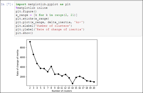
FIGURE 15-2: Rate of change of inertia for solutions up to k=20.
When examining inertia’s rate of change, look for jumps in the rate itself. If the rate jumps up, it means that adding a cluster more than the previous solution brings much more benefit than expected; if it jumps down instead, you’re likely forcing a cluster more than necessary. All the cluster solutions before a jump down may be a good candidate, according to the principle of parsimony (the jump signals a sophistication in our analysis, but the right solutions are usually the simplest). In the example, there are quite a few jumps at k=7, 9, 11, 14, 17 but k=17 seems to be the most promising peak because of a rate of change much higher with respect to the descending trend.
The rate of change in inertia will provide you with just a few tips where there could be good cluster solutions. It is up to you to decide which to pick if you need to get some extra insight on data. If, instead, clustering is just a step in a complex data science project, you don’t need to spend much effort in looking for an optimal number of clusters; you just pass a solution featuring enough clusters to the next machine learning algorithm and let it decide for the best.
Clustering big data
K-means is a way to reduce the complexity of your data by summarizing the many examples in your dataset. To perform this task, you load the data into your computer’s memory, and that won’t always be feasible, especially if you are working with big data. Scikit-learn offers an alternative way to apply K-means; the MiniBatchKMeans is a variant that can progressively cluster separated chunks of data. In fact, a batch learning procedure usually processes the data part by part. There are only two differences between the standard K-means function and MiniBatchKMeans:
- You cannot automatically test different starting centroids unless you try running the analysis again.
- The analysis will start when there is a batch made of at least a minimum number of cases. This value is usually set to 100 (but the more cases there are, the better the result) by the
batch_sizeparameter.
A simple demonstration on the previous handwritten dataset shows how effective and easy it is to use the MiniBatchKMeans clustering class. First, the example runs a test on the K-means algorithm on all the data available and records the inertia of the solution:
k = 10
clustering = KMeans(n_clusters=k,
n_init=10, random_state=1)
clustering.fit(Cx)
kmeans_inertia = clustering.inertia_
print("K-means inertia: %0.1f" % kmeans_inertia)
Take note that the resulting inertia is 58253.3. The example then tests the same data and number of clusters by fitting a MiniBatchKMeans clustering by small separate batches of 100 examples:
from sklearn.cluster import MiniBatchKMeans
batch_clustering = MiniBatchKMeans(n_clusters=k,
random_state=1)
batch = 100
for row in range(0, len(Cx), batch):
if row+batch < len(Cx):
feed = Cx[row:row+batch,:]
else:
feed = Cx[row:,:]
batch_clustering.partial_fit(feed)
batch_inertia = batch_clustering.score(Cx) * -1
print("MiniBatchKmeans inertia: %0.1f" % batch_inertia)
This script iterates through the indexes of the previously scaled and PCA simplified dataset (Cx), creating batches of 100 observations each. Using the partial_fit method, it fits a K-means clustering on each batch, using the centroids found by the previous call. The algorithm stops when it runs out of data. Using the score method on all the data available, it then reports its inertia for a 10-clusters solution. Now the reported inertia is 64633.6. Note that MiniBatchKmeans results in a higher inertia than the standard algorithm. Though the difference is minimal, the fitted solution is pejorative, thus you should reserve this approach for those times when you really cannot work with in-memory datasets.
Performing Hierarchical Clustering
If the K-means algorithm is concerned with centroids, hierarchical (also known as agglomerative) clustering tries to link each data point, by a distance measure, to its nearest neighbor, creating a cluster. Reiterating the algorithm using different linkage methods, the algorithm gathers all the available points into a rapidly diminishing number of clusters, until in the end all the points reunite into a single group.
The results, if visualized, will closely resemble the biological classifications of living beings that you may have studied in school or seen on posters at the local natural history museum, an upside-down tree whose branches are all converging into a trunk. Such a figurative tree is a dendrogram, and you see it used in medical and biological research. Scikit-learn implementation of agglomerative clustering does not offer the possibility of depicting a dendrogram from your data because such a visualization technique works fine with only a few cases, whereas you can expect to work on many examples.
Compared to K-means, agglomerative algorithms are more cumbersome and do not scale well to large datasets. Agglomerative algorithms are more suitable for statistical studies (they can be easily found in natural sciences, archeology, and sometimes psychology and economics). These algorithms do offer the advantage of creating a complete range of nested cluster solutions, so you just need to pick the right one for your purpose.
To use agglomerative clustering effectively, you have to know about the different linkage methods (the heuristics for clustering) and the distance metrics. There are three linkage methods:
- Ward: Tends to look for spherical clusters, very cohesive inside and extremely differentiated from other groups. Another nice characteristic is that the method tends to find clusters of similar size. It works only with the Euclidean distance.
- Complete: Links clusters using their furthest observations, that is, their most dissimilar data points. Consequently, clusters created using this method tend to be comprised of highly similar observations, making the resulting groups quite compact.
- Average: Links clusters using their centroids and ignoring their boundaries. The method creates larger groups than the complete method. In addition, the clusters can be of different sizes and shapes, contrary to the Ward’s solutions. Consequently, this approach sees successful use in the field of biological sciences, easily catching natural diversity.
There are also three distance metrics:
- Euclidean (euclidean or l2): As seen in K-means.
- Manhattan (manhattan or l1): Similar to Euclidean, but the distance is calculated by summing the absolute value of the difference between the dimensions. In a map, if the Euclidean distance is the shortest route between two points, the Manhattan distance implies moving straight, first along one axis and then along the other — as a car in the city would, reaching a destination by driving along city blocks (the distance is also known as city block distance).
- Cosine (cosine): A good choice when there are too many variables and you worry that some variable may not be significant (being just noise). Cosine distance reduces noise by taking the shape of the variables, more than their values, into account. It tends to associate observations that have the same maximum and minimum variables, regardless of their effective value.
Using a hierarchical cluster solution
If your dataset doesn’t contain too many observations, it’s worth trying agglomerative clustering with all the combinations of linkage and distance and then comparing the results carefully. In clustering, you rarely already know the right answers, and agglomerative clustering can provide you with another useful potential solution. For example, you can recreate the previous analysis with K-means and handwritten digits, using the ward linkage and the Euclidean distance as follows (the output appears in Figure 15-3):
from sklearn.cluster import AgglomerativeClustering
Hclustering = AgglomerativeClustering(n_clusters=10,
affinity='euclidean',
linkage='ward')
Hclustering.fit(Cx)
ms = np.column_stack((ground_truth,Hclustering.labels_))
df = pd.DataFrame(ms,
columns = ['Ground truth','Clusters'])
pd.crosstab(df['Ground truth'],
df['Clusters'], margins=True)

FIGURE 15-3: Cross-tabulation of ground truth and Ward’s agglomerative clusters.
The results, in this case, are slightly better than K-means, although, you may have noticed that completing the analysis using this approach certainly takes longer than using K-means. When working with a large number of observations, the computations for a hierarchical cluster solution may take hours to complete, making this solution less feasible. You can get around the time issue by using a two-phase clustering, which is faster and provides you with a hierarchical solution even when you are working with large datasets.
Using a two-phase clustering solution
To implement the two-phase clustering solution, you process the original observations using K-means with a large number of clusters. A good rule of thumb is to take the square root of the number of observations and use that figure; moreover, you always have to keep the number of clusters from exceeding the range of 100–200 for the second phase, based on hierarchical clustering, to work well. The following example uses 50 clusters.
from sklearn.cluster import KMeans
clustering = KMeans(n_clusters=50,
n_init=10,
random_state=1)
clustering.fit(Cx)
At this point, the tricky part is to keep track of what case has been assigned to what cluster derived from K-means. We use a dictionary for such a purpose.
Kx = clustering.cluster_centers_
Kx_mapping = {case:cluster for case,
cluster in enumerate(clustering.labels_)}
The new dataset is Kx, which is made up of the cluster centroids that the K-means algorithm has discovered. You can think of each cluster as a well-represented summary of the original data. If you cluster the summary now, it will be almost the same as clustering the original data.
from sklearn.cluster import AgglomerativeClustering
Hclustering = AgglomerativeClustering(n_clusters=10,
affinity='cosine',
linkage='complete')
Hclustering.fit(Kx)
You now map the results to the centroids you originally used so that you can easily determine whether a hierarchical cluster is made of certain K-means centroids. The result consists of the observations making up the K-means clusters having those centroids.
H_mapping = {case:cluster for case,
cluster in enumerate(Hclustering.labels_)}
final_mapping = {case:H_mapping[Kx_mapping[case]]
for case in Kx_mapping}
Now you can evaluate the solution you obtained using a similar confusion matrix as you did before for both K-means and hierarchical clustering (see Figure 15-4 for the results).
ms = np.column_stack((ground_truth,
[final_mapping[n] for n in range(max(final_mapping)+1)]))
df = pd.DataFrame(ms,
columns = ['Ground truth','Clusters'])
pd.crosstab(df['Ground truth'],
df['Clusters'], margins=True)
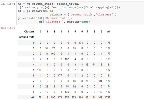
FIGURE 15-4: Cross-tabulation of ground truth and two-step clustering.
The solution you obtain is somehow analogous to the previous solutions. The result proves that this approach is a viable method for handling large datasets or even big data datasets, reducing them to a smaller representations and then operating with less scalable clustering, but more varied and precise techniques. The two-phase approach also presents another advantage because it operates well with noisy or outlying data — the initial K-means phase filters out such problems well and relegates them to separate cluster solutions.
Discovering New Groups with DBScan
Both K-means and agglomerative clustering, especially if you are using the Ward’s linkage criteria, will produce cohesive groups, similar to bubbles, equally spread in all directions. Reality can sometimes produce complex and unsettling results — groups may have strange forms far from the canonical bubble. The Scikit-learns’s datasets module (see http://scikit-learn.org/stable/modules/clustering.html for an overview) offers a wide range of mind-teasing shapes that you can’t successfully crunch using either K-means or agglomerative clustering: large circles containing smaller ones, interleaved small circles, and spiraling Swiss roll datasets (named after the sponge cake roll because of how the data points are arranged).
DBScan is another clustering algorithm based on a smart intuition that can solve even the most difficult problems. DBScan relies on the idea that clusters are dense, so to start exploring the data space in every direction and mark a cluster boundary when the density decreases should be sufficient. Areas of the data space with insufficient density of points are just considered empty, and all the points there are noise or outliers, that is, points characterized by unusual or strange values.
DBScan is more complex and requires more running time than K-means (but it is faster than agglomerative clustering). It automatically guesses the number of clusters and points out strange data that doesn’t easily fit into any class. This makes DBScan different from the previous algorithms that try to force every observation into a class.
Replicating the handwritten digit clustering requires just a few lines of Python code:
from sklearn.cluster import DBSCAN
DB = DBSCAN(eps=3.7, min_samples=15)
DB.fit(Cx)
Using DBScan, you won’t have to set a K number of expected clusters; the algorithm will find them by itself. Apparently, the lack of a K number seems to simplify the usage of DBScan; in reality, the algorithm requires you to fix two essential parameters, eps and min_sample, in order to work properly:
eps: The maximum distance between two observations that allows them to be part of the same neighborhood.min_sample: The minimum number of observations in a neighborhood that transform them into a core point.
The algorithm works by walking around the data and building clusters by linking observations arranged into neighborhoods. A neighborhood is a small cluster of data points all within a distance value of eps. If the number of points in the neighborhood is less than the number min_sample, then DBScan doesn’t form the neighborhood.
No matter what the shape of the cluster, DBScan links all the neighborhoods together if they are near enough (under the distance value of eps). When no more neighborhoods are within reach, DBScan tries to aggregate to group even single data points, if they are within eps distance. The data points that aren’t associated with any group are treated as noisy points (being too particular to be part of a group).
Try many values of eps and min_sample. The resulting clusters may also change drastically with respect to the values set into these two parameters. Start with a low number of min_samples. Using a lower number allows many neighborhoods to cluster together. The default number 5 is fine. Then try different numbers for eps, starting from 0.1 upward. Don’t be disappointed if you can’t get a viable result initially — keep trying different combinations.
Getting back to the example, after this brief explanation of DBScan details, some data exploration can allow you to observe the results under the right point of view. First, count the clusters:
from collections import Counter
print('No. clusters: %i' % len(np.unique(DB.labels_)))
print(Counter(DB.labels_))
ms = np.column_stack((ground_truth, DB.labels_))
df = pd.DataFrame(ms,
columns = ['Ground truth', 'Clusters'])
pd.crosstab(df['Ground truth'],
df['Clusters'], margins=True)
Almost half the observations are assigned to the cluster labeled -1, which represents the noise (noise is defined as examples that are too unusual to group). Given the number of dimensions (30 uncorrelated variables from a PCA analysis) in the data and its high variability (they are handwritten samples), many cases do not naturally fall together into the same group. Figure 15-5 shows the output from this example.
No. clusters: 12
Counter({-1: 836, 6: 182, 0: 172, 2: 159, 1: 156, 4: 119,
5: 77, 3: 28, 10: 21, 7: 18, 8: 16, 9: 13})
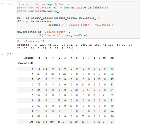
FIGURE 15-5: Cross-tabulation of ground truth and DBScan.
The strength of DBScan is to provide reliable, consistent clusters. DBScan isn’t forced, as are K-means and agglomerative clustering, to reach a solution with a certain number of clusters, even when such a solution does not exist.