
Chapter 6
Working with Real Data
IN THIS CHAPTER
![]() Manipulating data streams
Manipulating data streams
![]() Working with flat and unstructured files
Working with flat and unstructured files
![]() Interacting with relational databases
Interacting with relational databases
![]() Using NoSQL as a data source
Using NoSQL as a data source
![]() Interacting with web-based data
Interacting with web-based data
Data science applications require data by definition. It would be nice if you could simply go to a data store somewhere, purchase the data you need in an easy-open package, and then write an application to access that data. However, data is messy. It appears in all sorts of places, in many different forms, and you can interpret it in many different ways. Every organization has a different method of viewing data and stores it in a different manner as well. Even when the data management system used by one company is the same as the data management system used by another company, the chances are slim that the data will appear in the same format or even use the same data types. In short, before you can do any data science work, you must discover how to access the data in all its myriad forms. Real data requires a lot of work to use and fortunately, Python is up to the task of manipulating it as needed.
This chapter helps you understand the techniques required to access data in a number of forms and locations. For example, memory streams represent a form of data storage that your computer supports natively; flat files exist on your hard drive; relational databases commonly appear on networks (although smaller relational databases, such as those found in Access, could appear on your hard drive as well); and web-based data usually appears on the Internet. You won’t visit every form of data storage available (such as that stored on a point-of-sale, or POS, system). Quite possibly, an entire book on the topic wouldn’t suffice to cover the topic of data formats in any detail. However, the techniques in this chapter do demonstrate how to access data in the formats you most commonly encounter when working with real-world data.
 The Scikit-learn library includes a number of toy datasets (small datasets meant for you to play with). These datasets are complex enough to perform a number of tasks, such as experimenting with Python to perform data science tasks. Because this data is readily available, and making the examples too complicated to understand is a bad idea, this book relies on these toy datasets as input for many of the examples. Even though the book does use these toy datasets for the sake of reducing complexity and making the examples clearer, the techniques that the book demonstrates work equally well on real-world data that you access using the techniques shown in this chapter.
You don’t have to type the source code for this chapter in by hand. In fact, it’s a lot easier if you use the downloadable source (see the Introduction for download instructions). The source code for this chapter appears in the P4DS4D2_06_Dataset_Load.ipynb source code file.
 It’s essential that the
 Colors.txt, Titanic.csv, Values.xls, Colorblk.jpg, and XMLData.xml files that come with the downloadable source code appear in the same folder (directory) as your Notebook files. Otherwise, the examples in the following sections fail with an input/output (IO) error. The file location varies according to the platform you’re using. For example, on a Windows system, you find the notebooks stored in the C:UsersUsernameP4DS4D2 folder, where Username is your login name. (The book assumes that you’ve used the prescribed folder location of P4DS4D2, as described in the “Defining the code repository” section of Chapter 3.) To make the examples work, simply copy the four files from the downloadable source folder into your Notebook folder.
Uploading, Streaming, and Sampling Data
Storing data in local computer memory represents the fastest and most reliable means to access it. The data could reside anywhere. However, you don’t actually interact with the data in its storage location. You load the data into memory from the storage location and then interact with it in memory. This is the technique the book uses to access all the toy datasets found in the Scikit-learn library, so you see this technique used relatively often in the book.
 Data scientists call the columns in a database features or variables. The rows are cases. Each row represents a collection of variables that you can analyze.
Uploading small amounts of data into memory
The most convenient method that you can use to work with data is to load it directly into memory. This technique shows up a couple of times earlier in the book but uses the toy dataset from the Scikit-learn library. This section uses the Colors.txt file, shown in Figure 6-1, for input.

FIGURE 6-1: Format of the Colors.txt file.
The example also relies on native Python functionality to get the task done. When you load a file (of any type), the entire dataset is available at all times and the loading process is quite short. Here is an example of how this technique works.
with open("Colors.txt", 'r') as open_file:
    print('Colors.txt content:
' + open_file.read())
The example begins by using the open() method to obtain a file object. The open() function accepts the filename and an access mode. In this case, the access mode is read (r). It then uses the read() method of the file object to read all the data in the file. If you were to specify a size argument as part of read(), such as read(15), Python would read only the number of characters that you specify or stop when it reaches the End Of File (EOF). When you run this example, you see the following output:
Colors.txt content:
Color Value
Red 1
Orange 2
Yellow 3
Green 4
Blue 5
Purple 6
Black 7
White 8
The entire dataset is loaded from the library into free memory. Of course, the loading process will fail if your system lacks sufficient memory to hold the dataset. When this problem occurs, you need to consider other techniques for working with the dataset, such as streaming it or sampling it. In short, before you use this technique, you must ensure that the dataset will actually fit in memory. You won’t normally experience any problems when working with the toy datasets in the Scikit-learn library.
Streaming large amounts of data into memory
Some datasets will be so large that you won’t be able to fit them entirely in memory at one time. In addition, you may find that some datasets load slowly because they reside on a remote site. Streaming answers both needs by making it possible to work with the data a little at a time. You download individual pieces, making it possible to work with just part of the data and to work with it as you receive it, rather than waiting for the entire dataset to download. Here’s an example of how you can stream data using Python:
with open("Colors.txt", 'r') as open_file:
for observation in open_file:
print('Reading Data: ' + observation)
This example relies on the Colors.txt file, which contains a header, and then a number of records that associate a color name with a value. The open_file file object contains a pointer to the open file.
As the code performs data reads in the for loop, the file pointer moves to the next record. Each record appears one at a time in observation. The code outputs the value in observation using a print statement. You should receive this output:
Reading Data: Color Value
Reading Data: Red 1
Reading Data: Orange 2
Reading Data: Yellow 3
Reading Data: Green 4
Reading Data: Blue 5
Reading Data: Purple 6
Reading Data: Black 7
Reading Data: White 8
Python streams each record from the source. This means that you must perform a read for each record you want.
Generating variations on image data
At times, you need to import and analyze image data. The source and type of the image does make a difference. You see a number of examples of working with images throughout the book. However, a good starting point is to simply read a local image in, obtain statistics about that image, and display the image onscreen, as shown in the following code:
import matplotlib.image as img
import matplotlib.pyplot as plt
%matplotlib inline
image = img.imread("Colorblk.jpg")
print(image.shape)
print(image.size)
plt.imshow(image)
plt.show()
The example begins by importing two matplotlib libraries, image and pyplot. The image library reads the image into memory, while the pyplot library displays it onscreen.
After the code reads the file, it begins by displaying the image shape property — the number of horizontal pixels, vertical pixels, and pixel depth. Figure 6-2 shows that the image is 100 x 100 x 3 pixels. The image size property is the combination of these three elements, or 30,000 bytes.
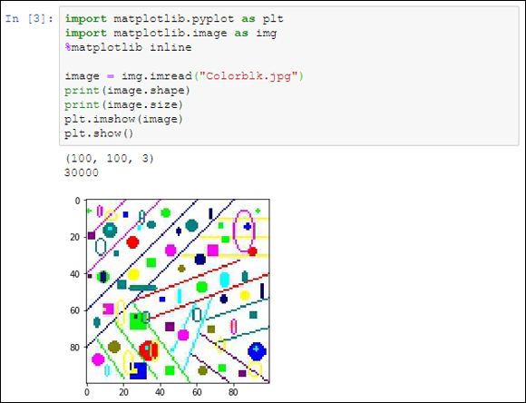
FIGURE 6-2: The test image is 100 pixels high and 100 pixels long.
The next step is to load the image for plotting using imshow(). The final call, plt.show(), displays the image onscreen, as shown in Figure 6-2. This technique represents just one of a number of methods for interacting with images using Python so that you can analyze them in some manner.
Sampling data in different ways
Data streaming obtains all the records from a data source. You may find that you don’t need all the records. You can save time and resources by simply sampling the data. This means retrieving records a set number of records apart, such as every fifth record, or by making random samples. The following code shows how to retrieve every other record in the Colors.txt file:
n = 2
with open("Colors.txt", 'r') as open_file:
for j, observation in enumerate(open_file):
if j % n==0:
print('Reading Line: ' + str(j) +
' Content: ' + observation)
The basic idea of sampling is the same as streaming. However, in this case, the application uses enumerate() to retrieve a row number. When j % n == 0, the row is one that you want to keep and the application outputs the information. In this case, you see the following output:
Reading Line: 0 Content: Color Value
Reading Line: 2 Content: Orange 2
Reading Line: 4 Content: Green 4
Reading Line: 6 Content: Purple 6
Reading Line: 8 Content: White 8
The value of n is important in determining which records appear as part of the dataset. Try changing n to 3. The output will change to sample just the header and rows 3 and 6.
You can perform random sampling as well. All you need to do is randomize the selector, like this:
from random import random
sample_size = 0.25
with open("Colors.txt", 'r') as open_file:
for j, observation in enumerate(open_file):
if random()<=sample_size:
print('Reading Line: ' + str(j) +
' Content: ' + observation)
To make this form of selection work, you must import the random class. The random() method outputs a value between 0 and 1. However, Python randomizes the output so that you don’t know what value you receive. The sample_size variable contains a number between 0 and 1 to determine the sample size. For example, 0.25 selects 25 percent of the items in the file.
The output will still appear in numeric order. For example, you won’t see Green come before Orange. However, the items selected are random, and you won’t always get precisely the same number of return values. The spaces between return values will differ as well. Here is an example of what you might see as output (although your output will likely vary):
Reading Line: 1 Content: Red 1
Reading Line: 4 Content: Green 4
Reading Line: 8 Content: White 8
Accessing Data in Structured Flat-File Form
In many cases, the data you need to work with won’t appear within a library, such as the toy datasets in the Scikit-learn library. Real-world data usually appears in a file of some type. A flat file presents the easiest kind of file to work with. The data appears as a simple list of entries that you can read one at a time, if desired, into memory. Depending on the requirements for your project, you can read all or part of the file.
A problem with using native Python techniques is that the input isn’t intelligent. For example, when a file contains a header, Python simply reads it as yet more data to process, rather than as a header. You can’t easily select a particular column of data. The pandas library used in the sections that follow makes it much easier to read and understand flat-file data. Classes and methods in the pandas library interpret (parse) the flat-file data to make it easier to manipulate.
The least formatted and therefore easiest-to-read flat-file format is the text file. However, a text file also treats all data as strings, so you often have to convert numeric data into other forms. A comma-separated value (CSV) file provides more formatting and more information, but it requires a little more effort to read. At the high end of flat-file formatting are custom data formats, such as an Excel file, which contains extensive formatting and could include multiple datasets in a single file.
The following sections describe these three levels of flat-file dataset and show how to use them. These sections assume that the file structures the data in some way. For example, the CSV file uses commas to separate data fields. A text file might rely on tabs to separate data fields. An Excel file uses a complex method to separate data fields and to provide a wealth of information about each field. You can work with unstructured data as well, but working with structured data is much easier because you know where each field begins and ends.
Reading from a text file
Text files can use a variety of storage formats. However, a common format is to have a header line that documents the purpose of each field, followed by another line for each record in the file. The file separates the fields using tabs. Refer to Figure 6-1 for an example of the Colors.txt file used for the example in this section.
Native Python provides a wide variety of methods you can use to read such a file. However, it’s far easier to let someone else do the work. In this case, you can use the pandas library to perform the task. Within the pandas library, you find a set of parsers, code used to read individual bits of data and determine the purpose of each bit according to the format of the entire file. Using the correct parser is essential if you want to make sense of file content. In this case, you use the read_table() method to accomplish the task, as shown in the following code:
import pandas as pd
color_table = pd.io.parsers.read_table("Colors.txt")
print(color_table)
The code imports the pandas library, uses the read_table() method to read Colors.txt into a variable named color_table, and then displays the resulting memory data onscreen using the print function. Here’s the output you can expect to see from this example.
Color Value
0 Red 1
1 Orange 2
2 Yellow 3
3 Green 4
4 Blue 5
5 Purple 6
6 Black 7
7 White 8
Notice that the parser correctly interprets the first row as consisting of field names. It numbers the records from 0 through 7. Using read_table() method arguments, you can adjust how the parser interprets the input file, but the default settings usually work best. You can read more about the read_table() arguments at http://pandas.pydata.org/pandas-docs/version/0.23.0/generated/pandas.read_table.html.
Reading CSV delimited format
A CSV file provides more formatting than a simple text file. In fact, CSV files can become quite complicated. There is a standard that defines the format of CSV files, and you can see it at https://tools.ietf.org/html/rfc4180. The CSV file used for this example is quite simple:
- A header defines each of the fields
- Fields are separated by commas
- Records are separated by linefeeds
- Strings are enclosed in double quotes
- Integers and real numbers appear without double quotes
Figure 6-3 shows the raw format for the Titanic.csv file used for this example. You can see the raw format using any text editor.

FIGURE 6-3: The raw format of a CSV file is still text and quite readable.
Applications such as Excel can import and format CSV files so that they become easier to read. Figure 6-4 shows the same file in Excel.

FIGURE 6-4: Use an application such as Excel to create a formatted CSV presentation.
Excel actually recognizes the header as a header. If you were to use features such as data sorting, you could select header columns to obtain the desired result. Fortunately, pandas also makes it possible to work with the CSV file as formatted data, as shown in the following example:
import pandas as pd
titanic = pd.io.parsers.read_csv("Titanic.csv")
X = titanic[['age']]
print(X)
Notice that the parser of choice this time is read_csv(), which understands CSV files and provides you with new options for working with it. (You can read more about this parser at http://pandas.pydata.org/pandas-docs/version/0.23.0/generated/pandas.read_csv.html.) Selecting a specific field is quite easy — you just supply the field name as shown. The output from this example looks like this (some values omitted for the sake of space):
age
0 29.0000
1 0.9167
2 2.0000
3 30.0000
4 25.0000
5 48.0000
…
1304 14.5000
1305 9999.0000
1306 26.5000
1307 27.0000
1308 29.0000
[1309 rows x 1 columns]
Of course, a human readable output like this one is nice when working through an example, but you might also need the output as a list. To create the output as a list, you simply change the third line of code to read X = titanic[[’age’]].values. Notice the addition of the values property. The output changes to something like this (some values omitted for the sake of space):
[[ 29. ]
[ 0.91670001]
[ 2. ]
…,
[ 26.5 ]
[ 27. ]
[ 29. ]]
Reading Excel and other Microsoft Office files
Excel and other Microsoft Office applications provide highly formatted content. You can specify every aspect of the information these files contain. The Values.xls file used for this example provides a listing of sine, cosine, and tangent values for a random list of angles. You can see this file in Figure 6-5.
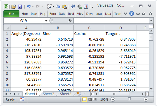
FIGURE 6-5: An Excel file is highly formatted and might contain information of various types.
When you work with Excel or other Microsoft Office products, you begin to experience some complexity. For example, an Excel file can contain more than one worksheet, so you need to tell pandas which worksheet to process. In fact, you can choose to process multiple worksheets, if desired. When working with other Office products, you have to be specific about what to process. Just telling pandas to process something isn’t good enough. Here’s an example of working with the Values.xls file.
import pandas as pd
xls = pd.ExcelFile("Values.xls")
trig_values = xls.parse('Sheet1', index_col=None,
na_values=['NA'])
print(trig_values)
The code begins by importing the pandas library as normal. It then creates a pointer to the Excel file using the ExcelFile() constructor. This pointer, xls, lets you access a worksheet, define an index column, and specify how to present empty values. The index column is the one that the worksheet uses to index the records. Using a value of None means that pandas should generate an index for you. The parse() method obtains the values you request. You can read more about the Excel parser options at https://pandas.pydata.org/pandas-docs/stable/generated/pandas.ExcelFile.parse.html.
You don’t absolutely have to use the two-step process of obtaining a file pointer and then parsing the content. You can also perform the task using a single step like this: trig_values = pd.read_excel("Values.xls", ’Sheet1’, index_col=None, na_values=[’NA’]). Because Excel files are more complex, using the two-step process is often more convenient and efficient because you don’t have to reopen the file for each read of the data.
Sending Data in Unstructured File Form
Unstructured data files consist of a series of bits. The file doesn’t separate the bits from each other in any way. You can’t simply look into the file and see any structure because there isn’t any to see. Unstructured file formats rely on the file user to know how to interpret the data. For example, each pixel of a picture file could consist of three 32-bit fields. Knowing that each field is 32-bits is up to you. A header at the beginning of the file may provide clues about interpreting the file, but even so, it’s up to you to know how to interact with the file.
The example in this section shows how to work with a picture as an unstructured file. The example image is a public domain offering from http://commons.wikimedia.org/wiki/Main_Page. To work with images, you need to access the Scikit-image library (http://scikit-image.org/), which is a free-of-charge collection of algorithms used for image processing. You can find a tutorial for this library at http://scipy-lectures.github.io/packages/scikit-image/. The first task is to be able to display the image onscreen using the following code. (This code can require a little time to run. The image is ready when the busy indicator disappears from the Notebook tab.)
from skimage.io import imread
from skimage.transform import resize
from matplotlib import pyplot as plt
import matplotlib.cm as cm
example_file = ("http://upload.wikimedia.org/" +
"wikipedia/commons/7/7d/Dog_face.png")
image = imread(example_file, as_grey=True)
plt.imshow(image, cmap=cm.gray)
plt.show()
The code begins by importing a number of libraries. It then creates a string that points to the example file online and places it in example_file. This string is part of the imread() method call, along with as_grey, which is set to True. The as_grey argument tells Python to turn any color images into gray scale. Any images that are already in gray scale remain that way.
Now that you have an image loaded, it’s time to render it (make it ready to display onscreen. The imshow() function performs the rendering and uses a grayscale color map. The show() function actually displays image for you, as shown in Figure 6-6.
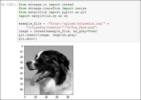
FIGURE 6-6: The image appears onscreen after you render and show it.
You now have an image in memory and you may want to find out more about it. When you run the following code, you discover the image type and size:
print("data type: %s, shape: %s" %
(type(image), image.shape))
The output from this call tells you that the image type is a numpy.ndarray and that the image size is 90 pixels by 90 pixels. The image is actually an array of pixels that you can manipulate in various ways. For example, if you want to crop the image, you can use the following code to manipulate the image array:
image2 = image[5:70,0:70]
plt.imshow(image2, cmap=cm.gray)
plt.show()
The numpy.ndarray in image2 is smaller than the one in image, so the output is smaller as well. Figure 6-7 shows typical results. The purpose of cropping the image is to make it a specific size. Both images must be the same size for you to analyze them. Cropping is one way to ensure that the images are the correct size for analysis.
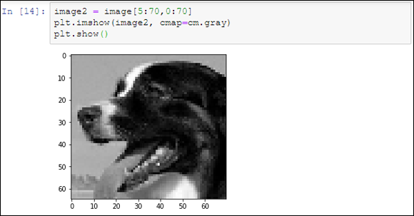
FIGURE 6-7: Cropping the image makes it smaller.
Another method that you can use to change the image size is to resize it. The following code resizes the image to a specific size for analysis:
image3 = resize(image2, (30, 30), mode='symmetric')
plt.imshow(image3, cmap=cm.gray)
print("data type: %s, shape: %s" %
(type(image3), image3.shape))
The output from the print() function tells you that the image is now 30 pixels by 30 pixels in size. You can compare it to any image with the same dimensions.
After you have all the images the right size, you need to flatten them. A dataset row is always a single dimension, not two dimensions. The image is currently an array of 30 pixels by 30 pixels, so you can’t make it part of a dataset. The following code flattens image3 so that it becomes an array of 900 elements that is stored in image_row.
image_row = image3.flatten()
print("data type: %s, shape: %s" %
(type(image_row), image_row.shape))
Notice that the type is still a numpy.ndarray. You can add this array to a dataset and then use the dataset for analysis purposes. The size is 900 elements, as anticipated.
Managing Data from Relational Databases
Databases come in all sorts of forms. For example, AskSam (http://asksam.en.softonic.com/) is a kind of free-form textual database. However, the vast majority of data used by organizations rely on relational databases because these databases provide the means for organizing massive amounts of complex data in an organized manner that makes the data easy to manipulate. The goal of a database manager is to make data easy to manipulate. The focus of most data storage is to make data easy to retrieve.
Relational databases accomplish both the manipulation and data retrieval objectives with relative ease. However, because data storage needs come in all shapes and sizes for a wide range of computing platforms, there are many different relational database products. In fact, for the data scientist, the proliferation of different Database Management Systems (DBMSs) using various data layouts is one of the main problems you encounter with creating a comprehensive dataset for analysis.
The one common denominator between many relational databases is that they all rely on a form of the same language to perform data manipulation, which does make the data scientist’s job easier. The Structured Query Language (SQL) lets you perform all sorts of management tasks in a relational database, retrieve data as needed, and even shape it in a particular way so that the need to perform additional shaping is unnecessary.
Creating a connection to a database can be a complex undertaking. For one thing, you need to know how to connect to that particular database. However, you can divide the process into smaller pieces. The first step is to gain access to the database engine. You use two lines of code similar to the following code (but the code presented here is not meant to execute and perform a task):
from sqlalchemy import create_engine
engine = create_engine('sqlite:///:memory:')
After you have access to an engine, you can use the engine to perform tasks specific to that DBMS. The output of a read method is always a DataFrame object that contains the requested data. To write data, you must create a DataFrame object or use an existing DataFrame object. You normally use these methods to perform most tasks:
read_sql_table(): Reads data from a SQL table to aDataFrameobjectread_sql_query(): Reads data from a database using a SQL query to aDataFrameobjectread_sql(): Reads data from either a SQL table or query to aDataFrameobjectDataFrame.to_sql(): Writes the content of aDataFrameobject to the specified tables in the database
The sqlalchemy library provides support for a broad range of SQL databases. The following list contains just a few of them:
- SQLite
- MySQL
- PostgreSQL
- SQL Server
- Other relational databases, such as those you can connect to using Open Database Connectivity (ODBC)
You can discover more about working with databases at https://docs.sqlalchemy.org/en/latest/core/engines.html. The techniques that you discover in this book using the toy databases also work with relational databases.
Interacting with Data from NoSQL Databases
In addition to standard relational databases that rely on SQL, you find a wealth of databases of all sorts that don’t have to rely on SQL. These Not only SQL (NoSQL) databases are used in large data storage scenarios in which the relational model can become overly complex or can break down in other ways. The databases generally don’t use the relational model. Of course, you find fewer of these DBMSes used in the corporate environment because they require special handling and training. Still, some common DBMSes are used because they provide special functionality or meet unique requirements. The process is essentially the same for using NoSQL databases as it is for relational databases:
- Import required database engine functionality.
- Create a database engine.
- Make any required queries using the database engine and the functionality supported by the DBMS.
The details vary quite a bit, and you need to know which library to use with your particular database product. For example, when working with MongoDB (https://www.mongodb.org/), you must obtain a copy of the PyMongo library (https://api.mongodb.org/python/current/) and use the MongoClient class to create the required engine. The MongoDB engine relies heavily on the find() function to locate data. Following is a pseudo-code example of a MongoDB session. (You won’t be able to execute this code in Notebook; it’s shown only as an example.)
import pymongo
import pandas as pd
from pymongo import Connection
connection = Connection()
db = connection.database_name
input_data = db.collection_name
data = pd.DataFrame(list(input_data.find()))
Accessing Data from the Web
It would be incredibly difficult (perhaps impossible) to find an organization today that doesn’t rely on some sort of web-based data. Most organizations use web services of some type. A web service is a kind of web application that provides a means to ask questions and receive answers. Web services usually host a number of input types. In fact, a particular web service may host entire groups of query inputs.
Another type of query system is the microservice. Unlike the web service, microservices have a specific focus and provide only one specific query input and output. Using microservices has specific benefits that are outside the scope of this book to address, but essentially they work like tiny web services, so that’s how this book addresses them.
One of the most beneficial data access techniques to know when working with web data is accessing XML. All sorts of content types rely on XML, even some web pages. Working with web services and microservices means working with XML (in most cases). With this in mind, the example in this section works with XML data found in the XMLData.xml file, shown in Figure 6-8. In this case, the file is simple and uses only a couple of levels. XML is hierarchical and can become quite a few levels deep.

FIGURE 6-8: XML is a hierarchical format that can become quite complex.
The technique for working with XML, even simple XML, can be a bit harder than anything else you’ve worked with so far. Here’s the code for this example:
from lxml import objectify
import pandas as pd
xml = objectify.parse(open('XMLData.xml'))
root = xml.getroot()
df = pd.DataFrame(columns=('Number', 'String', 'Boolean'))
for i in range(0,4):
obj = root.getchildren()[i].getchildren()
row = dict(zip(['Number', 'String', 'Boolean'],
[obj[0].text, obj[1].text,
obj[2].text]))
row_s = pd.Series(row)
row_s.name = i
df = df.append(row_s)
print(df)
The example begins by importing libraries and parsing the data file using the objectify.parse() method. Every XML document must contain a root node, which is <MyDataset> in this case. The root node encapsulates the rest of the content, and every node under it is a child. To do anything practical with the document, you must obtain access to the root node using the getroot() method.
The next step is to create an empty DataFrame object that contains the correct column names for each record entry: Number, String, and Boolean. As with all other pandas data handling, XML data handling relies on a DataFrame. The for loop fills the DataFrame with the four records from the XML file (each in a <Record> node).
The process looks complex but follows a logical order. The obj variable contains all the children for one <Record> node. These children are loaded into a dictionary object in which the keys are Number, String, and Boolean to match the DataFrame columns.
There is now a dictionary object that contains the row data. The code creates an actual row for the DataFrame next. It gives the row the value of the current for loop iteration. It then appends the row to the DataFrame. To see that everything worked as expected, the code prints the result, which looks like this:
Number String Boolean
0 1 First True
1 2 Second False
2 3 Third True
3 4 Fourth False