
Chapter 4
Working with Google Colab
IN THIS CHAPTER
![]() Understanding Google Colab
Understanding Google Colab
![]() Accessing Google and Colab
Accessing Google and Colab
![]() Performing essential Colab tasks
Performing essential Colab tasks
![]() Obtaining additional information
Obtaining additional information
Colaboratory (https://colab.research.google.com/notebooks/welcome.ipynb), or Colab for short, is a Google cloud-based service that replicates Jupyter Notebook in the cloud. You don’t have to install anything on your system to use it. In most respects, you use Colab as you would a desktop installation of Jupyter Notebook (also called Notebook throughout the book). This book includes this chapter mainly for those readers who use something other than a standard desktop setup to work through the examples.
 Because you may not be using the same versions of products that appear in this book, the book’s example source code may or may not work precisely as described in the text when you use Colab. Also when using Colab, you may not see the results as presented in this book because of the differences in hardware between platforms. The introductory sections of this chapter go into more detail about Colab and help you understand what you can expect from it. However, the most important thing to remember is that Colab isn’t a replacement for Jupyter Notebook and the examples aren’t tested to specifically work with it, but you can try it with your alternative device if desired to follow the examples.
To use Colab, you must have a Google account and then access Colab using your account. Otherwise, most of the Colab features won’t work. The next section of the chapter gets you started with Google and helps you access Colab.
As with Notebook, you can use Colab to perform specific tasks in a cell-oriented paradigm. The next sections of the chapter go through a range of task-related topics that start with the use of notebooks. If you’ve used Notebook in previous chapters, you notice a strong resemblance between Notebook and Colab. Of course, you also want to perform other sorts of tasks, such as creating various cell types and using them to create notebooks that look like those you create with Notebook.
Finally, this chapter can’t address every aspect of Colab, so the final section of the chapter serves as a handy resource for locating the most reliable information about Colab.
Defining Google Colab
Google Colab is the cloud version of Notebook. In fact, the Welcome page makes this fact apparent. It even uses IPython (the previous name for Jupyter) Notebook (.ipynb) files for the site. That’s right, you’re viewing a Notebook right there in your browser. Even though the two applications are similar and they both use .ipynb files, they do have some differences that you need to know about. The following sections help you understand the Colab differences.
Understanding what Google Colab does
You can use Colab to perform many tasks, but for the purpose of this book, you use it to write and run code, create its associated documentation, and display graphics, just as you do with Notebook. The techniques you use are similar, in fact, to using Notebook, but later in the chapter, you find out the small differences between the two. Even so, the downloadable source for this book should run without much effort on your part.
Notebook is a localized application in that you use local resources with it. You could potentially use other sources, but doing so could prove inconvenient or impossible in some cases. For example, according to https://help.github.com/articles/working-with-jupyter-notebook-files-on-github/, your Notebook files will appear as static HTML pages when you use a GitHub repository. In fact, some features won’t work at all. Colab enables you to fully interact with your Notebook files using GitHub as a repository. In fact, Colab supports a number of online storage options, so you can regard Colab as your online partner in creating Python code.
The other reason that you really need to know about Colab is that you can use it with your alternative device. During the writing process, some of the example code was tested on an Android-based tablet (an ASUS ZenPad 3S 10). The target tablet has Chrome installed and executes the code well enough to follow the examples. All this said, you likely won’t want to try to write code using a tablet of that size — the text was incredibly small, for one thing, and the lack of a keyboard could be a problem, too. The point is that you don’t absolutely have to have a Windows, Linux, or OS X system to try the code, but the alternatives might not provide quite the performance you expect.
Google Colab generally doesn’t work with browsers other than Chrome or Firefox. In most cases, you see an error message and no other display if you try to start Colab in a browser that it doesn’t support. Your copy of Firefox may also need some configuration to work properly (see the “Using local runtime support” section, later in this chapter, for details). The amount of configuration that you perform depends on which Colab features you choose to use. Many examples work fine in Firefox without any modification.
Considering the online coding difference
For the most part, you use Colab just as you would Notebook. However, some features work differently. For example, to execute the code within a cell, you select that cell and click the run button (right-facing arrow) for that cell. The current cell remains selected, which means that you must actually initiate the selection of the next cell as a separate action. A block next to the output lets you clear just that output without affecting any other cell. Hovering the mouse over the block tells you when someone executed the content. On the right side of the cell, you see a vertical ellipsis that you can click to see a menu of options for that cell. The result is the same as when using Notebook, but the process for achieving the result is different.
The actual process for working with the code also differs from Notebook. Yes, you still type the code as you always have and the resulting code executes without problem in Notebook. The difference is in the way you can manage the code. You can upload code from your local drive as desired and then save it to a Google Drive or GitHub. The code becomes accessible from any device at this point by accessing those same sources. All you need to do is load Colab to access it.
If you use Chrome when working with Colab and choose to sync your copy of Chrome among various devices, all your code becomes available on any device you choose to work with. Syncing transfers your choices to all your devices as long as those devices are also set to synchronize their settings. Consequently, you can write code on your desktop, test it on your tablet, and then review it on your smart phone. It’s all the same code, all the same repository, and the same Chrome setup, just a different device.
What you may find, however, is that all this flexibility comes at the price of speed and ergonomics. In reviewing the various options, a local copy of Notebook executes the code in this book faster than a copy of Colab using any of the available configurations (even when working with a local copy of the .ipynb file). So, you trade speed for flexibility when working with Colab. In addition, viewing the source code on a tablet is hard; viewing it on a smart phone is nearly impossible. If you make the text large enough to see, you can’t see enough of the code to make any sort of reasonable editing possible. At best, you could review the code one line at a time to determine how it works.
 Using Notebook has other benefits, too. For example, when working with Colab, you have options to download your source files only as
 .ipynb or .py files. Colab doesn’t include all the other download options, including (but not limited to) HTML, LaTeX, and PDF. Consequently, your options for creating presentations from the online content are also limited to some extent. In short, using Colab and Notebook provides different coding experiences to some degree. They’re not mutually exclusive, however, because they share file formats. Theoretically, switching between the two as needed is possible.
One thing to consider when using Notebook and Colab is that the two products use most of the same terminology and many of the same features, but they’re not completely the same. The methods used to perform tasks differ, and some of the terminology does as well. For example, a Markdown cell in Notebook is a Text cell in Colab. The “Performing Common Tasks” section of this chapter tells you about other differences you need to consider.
Using local runtime support
The only time you really need local runtime support is when you want to work within a team environment and you need the speed or resource access advantage offered by a local runtime. Using a local runtime normally produces better speed than you obtain when relying on the cloud. In addition, a local runtime enables you to access files on your machine. A local runtime also gives you control over the version of Notebook used to execute code. You can read more about local runtime support at https://research.google.com/colaboratory/local-runtimes.html.
 You need to consider several issues when determining the need for local runtime support. The most obvious is that you need a local runtime, which means that this option won’t work with your laptop or tablet unless your laptop has Windows, Linux, or OS X and the appropriate version of Notebook installed. Your laptop or tablet will also need an appropriate browser; Internet Explorer is almost guaranteed to cause problems, assuming that it works at all.
The most important consideration when using a local runtime, however, is that your machine is now open to possible infection from Notebook code. You need to trust the party supplying the code. The local runtime option doesn’t open your machine to others that you share code with, however; they must either use their own local runtimes or rely on the cloud to execute code.
When working with Colab on using local runtime support and Firefox, you must perform some special setups. Make sure to read the Browser Specific Setups section on the Local Runtimes page to ensure that you have Firefox configured correctly. Always verify your setup. Firefox may appear to work correctly with Colab. However, a configuration issue arises when you perform tasks with it, and Colab shows error messages that say the code didn’t execute (or something else that isn’t particularly helpful).
Getting a Google Account
Before you can perform any significant tasks using Colab, you must have a Google account. You can use the same account for all sorts of purposes, not just development. For example, a Google account gives you access to Google Docs (https://www.google.com/docs/about/), an online document management system similar to Office 365.
Creating the account
To create a Google account, simply navigate to https://account.google.com/ and click the Create Your Google Account link. This page also contains a wealth of information about what a Google account can provide. When you click Create Your Google Account, you see the page shown in Figure 4-1. The account creation process consumes several pages. You just provide the required information in each page and click Next.

FIGURE 4-1: Follow the prompts to create your Google account.
Signing in
After you create and verify your account, you can sign into it. Before you can use Colab effectively, you must sign into your account. That’s because Colab relies on your Google Drive for certain tasks. You can also store notebooks in other places, such as GitHub, but having your Google account ensures that everything works as planned. To sign into your account, navigate to https://accounts.google.com/, provide your e-mail address and password, and then click Next. You see the sign-in page shown in Figure 4-2.
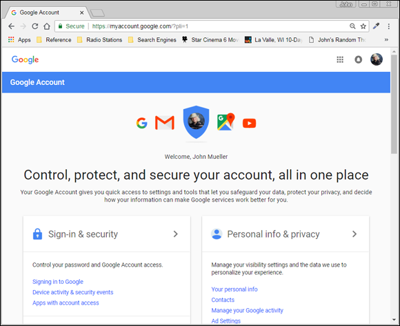
FIGURE 4-2: The sign-in page gives you access to all the general features, including your drive.
Working with Notebooks
As with Jupyter Notebook, the notebook forms the basis of interactions with Colab. In fact, Colab is built on notebooks, as previously mentioned. When you place the mouse on certain parts of the Welcome page at https://colab.research.google.com/notebooks/welcome.ipynb, you see opportunities for interacting with the page by adding either code or text entries (which you can use for notes as needed). These entries are active, so you can interact with them. You can also move cells around and copy the resulting material to your Google Drive. Of course, while interacting with the Welcome page is both unexpected and fun, the real purpose of this chapter is to demonstrate how to interact with Colab notebooks. The following sections describe how to perform basic notebook-related tasks with Colab.
Creating a new notebook
To create a new notebook, choose File ⇒ New Python 3 Notebook. You see a new Python 3 notebook like the one shown in Figure 4-3. The new notebook looks similar to, but not precisely the same as, those found in Notebook. However, all the same functionality exists. You can also create a new Python 2 notebook if desired, but this book doesn’t rely on Python 2.
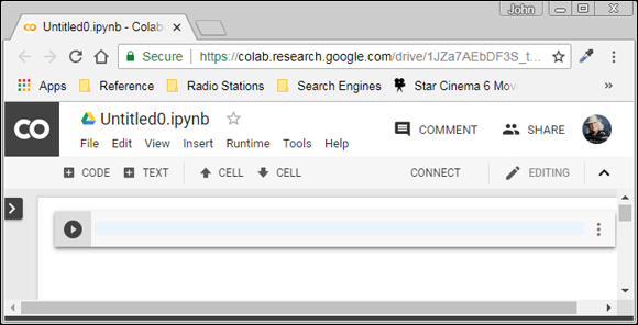
FIGURE 4-3: Create a new Python 3 Notebook using the same techniques as normal.
The notebook shown in Figure 4-3 lets you change the filename by clicking on it, just as you do when working in Notebook. Some features work differently but provide the same results. For example, to run the code in a particular cell, you click the right-pointing arrow on the left side of that cell. In contrast to Notebook, the cell focus doesn’t change to the next cell, so you must choose the next cell directly or by clicking the Next Cell or Previous Cell buttons on the toolbar.
Opening existing notebooks
You can open existing notebooks found in local storage, on Google Drive, or on GitHub. You can also open any of the Colab examples or upload files from sources that you can access, such as a network drive on your system. In all cases, you begin by choosing File ⇒ Open Notebook. You see the dialog box shown in Figure 4-4.
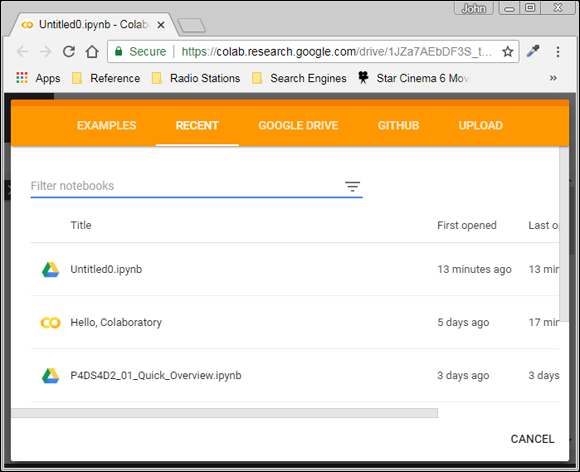
FIGURE 4-4: Use this dialog box to open existing notebooks.
The default view shows all the files you opened recently, regardless of location. The files appear in alphabetical order. You can filter the number of items displayed by typing a string into the Filter Notebooks field. Across the top are other options for opening notebooks.
Even if you’re not logged in, you can still access the Colab example projects. These projects help you understand Colab but won’t allow you to do anything with your own projects. Even so, you can still experiment with Colab without logging into Google first. The following sections discuss these options in more detail.
Using Google Drive for existing notebooks
Google Drive is the default location for many operations in Colab, and you can always choose it as a destination. When working with Drive, you see a list of files similar to those shown in Figure 4-4. To open a particular file, you click its link in the dialog box. The file opens in the current tab of your browser.
Using GitHub for existing notebooks
When working with GitHub, you initially need to provide the location of the source code online, as shown in Figure 4-5. The location must point to a public project; you can’t use Colab to access private projects.

FIGURE 4-5: When using GitHub, you must provide the location of the source code.
After you make the connection to GitHub, you see two lists: repositories, which are containers for code related to a particular project; and branches, a particular implementation of the code. Selecting a repository and branch displays a list of notebook files that you can load into Colab. Simply click the required link and it loads as if you were using a Google Drive.
Using local storage for existing notebooks
If you want to use the downloadable source for this book, or any local source for that matter, you select the Upload tab of the dialog box. In the center is a single button, Choose File. Clicking this button opens the File Open dialog box for your browser. You locate the file you want to upload, just as you normally would for opening any file.
Selecting a file and clicking Open uploads the file to Google Drive. If you make changes to the file, those changes appear on Google Drive, not on your local drive. Depending on your browser, you usually see a new window open with the code loaded. However, you could also simply see a success message, in which case you must now open the file using the same technique as you would when using Google Drive. In some case, your browser asks whether you want to leave the current page. You should tell the browser to do so.
The File ⇒ Upload Notebook command also uploads a file to Google Drive. In fact, uploading a notebook works like uploading any other kind of file, and you see the same dialog box. If you want to upload other kinds of files, using the File ⇒ Upload Notebook command is likely faster.
Saving notebooks
Colab provides a significant number of options for saving your notebook. However, none of these options works with your local drive. After you upload content from your local drive to Google Drive or GitHub, Colab manages the content in the cloud and not on your local drive. To save updates to your local drive, you must download the file using the techniques found in the “Downloading notebooks” section, later in this chapter. The following sections review the cloud-based options for saving notebooks.
Using Drive to save notebooks
The default location for storing your data is Google Drive. When you choose File ⇒ Save, the content you create goes to the root directory of your Google Drive. If you want to save the content to a different folder, you need to select that folder in Google Drive (https://drive.google.com/).
Colab tracks the versions of your project as you perform saves. However, as these revisions age, Colab removes them. To save a version that won’t age, you use the File ⇒ Save and Pin Revision command. To see the revisions for your project, choose File ⇒ Revision History. You see the output shown in Figure 4-6. Notice that the first entry is pinned. You can also pin entries by checking the entry in the History list. The revision history also shows you the modification date, who made the revision, and the size of the resulting file. You can use this list to restore a previous revision or download the revision to your local drive.
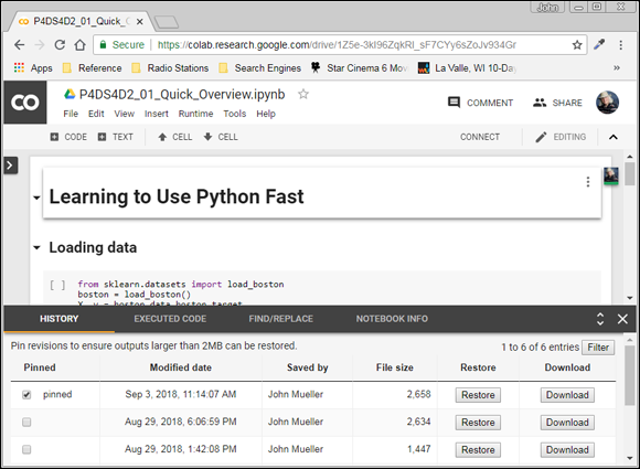
FIGURE 4-6: Colab maintains a history of the revisions for your project.
You can also save a copy of your project by choosing File ⇒ Save a Copy In Drive. The copy receives the word Copy as part of its name. Of course, you can rename it later. Colab stores the copy in the current Google Drive folder.
Using GitHub to save notebooks
GitHub provides an alternative to Google Drive for saving content. It offers an organized method of sharing code for the purpose of discussion, review, and distribution. You can find GitHub at https://github.com/.
You may use only public repositories when working with GitHub from Colab, even though GitHub also supports private repositories. To save a file to GitHub, choose File ⇒ Save a Copy in GitHub. If you aren’t already signed into GitHub, Colab displays a window that requests your sign-in information. After you sign in, you see a dialog box similar to the one shown in Figure 4-7.

FIGURE 4-7: Using GitHub means storing your data in a repository.
Notice that this account doesn’t currently have a repository. You must either create a new repository or choose an existing repository in which to store your data. After you save the file, it will appear in your GitHub repository of your choice. The repository will include a link to open the data in Colab by default, unless you choose not to include this feature.
Using GitHubGist to save notebooks
You use GitHub Gists as a means of sharing single files or other resources with other people. Some people use them for full projects as well, but the idea is that you have a concept that you want to share — something that isn’t quite fully formed and doesn’t represent a usable application. You can read more about Gists at https://help.github.com/articles/about-gists/.
As with GitHub, Gists come in both public and secret form. You can access both public and secret Gists from Colab, but Colab automatically keeps your files secret. To save your current project as a Gist, you choose File ⇒ Save a Copy as a GitHub Gist. Unlike GitHub, you don’t need to create a repository or do anything fancy in this case. The file saves as a Gist without any extra effort. The resulting entry always contains a View in Colaboratory link, as shown in Figure 4-8.
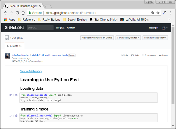
FIGURE 4-8: Use Gists to store individual files or other resources.
Downloading notebooks
Colab supports two methods for downloading notebooks to your local drive: .ipynb files (using File ⇒ Download .ipynb) and .py files (using File ⇒ Download .py). In both cases, the file appears in the default download directory for your browser; Colab doesn’t offer a method for downloading the file to a specific directory.
Performing Common Tasks
Most tasks in Colab work similar to their Notebook counterparts. For example, you can create code cells just as you do in Notebook. Markdown cells come in three forms: text, heading, and table of contents. They work somewhat differently from the Markdown cells found in Notebook, but the idea is the same. You can also edit and move cells, just as you do with Notebook. One important difference is that you can’t change a cell type. A cell that you create as a header can’t suddenly transform into a code cell. The following sections provide a brief overview of the various features.
Creating code cells
The first cell that Colab creates for you is a code cell. The code you create in Colab uses all the same features that you find in Notebook. However, off to the side of the cell, you see a menu of extras that you can use with Colab that aren’t present in Notebook, as shown in Figure 4-9.
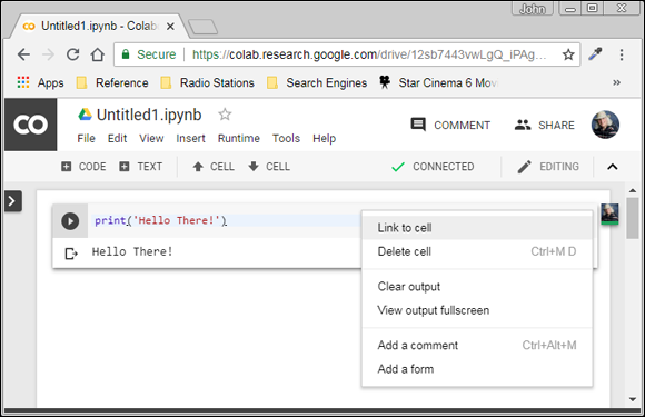
FIGURE 4-9: Colab code cells contain a few extras not found in Notebook.
You use the options shown in Figure 4-9 to augment your Colab code experience. The following list provides a short description of these features:
- Link to Cell: Displays a dialog box containing a link you can use to access a specific cell within the notebook. You can embed this link anywhere on a web page or within a notebook to allow someone to access that specific cell. The person still sees the entire notebook but doesn’t have to search for the cell you want to discuss.
- Delete Cell: Removes the cell from the notebook.
- Clear Output: Removes the output from the cell. You must run the code again to regenerate the output.
- View Output Fullscreen: Displays the output (not the entire cell or any other part of the notebook) in full-screen mode on the host device. This option is useful when displaying a significant amount of content or when a detailed view of graphics helps explain a topic. Press Esc to exit full-screen mode.
- Add a Comment: Creates a comment balloon to the right of the cell. This is not the same as a code comment, which exists in line with the code but affects the entire cell. You can edit, delete, or resolve comments. A resolved comment is one that receives attention and is no longer applicable.
- Add a Form: Inserts a form into the cell to the right of the code. You use forms to provide a graphical input for parameters. Forms don’t appear in Notebook, but because of how you create them, they won’t prevent you from running the code in Notebook. You can read more about forms at
https://colab.research.google.com/notebooks/forms.ipynb.
Code cells also tell you about the code and its execution. The little icon next to the output displays information about the execution when you hover your mouse over it, as shown in Figure 4-10. Clicking the icon clears the output. You must run the code again to regenerate the output.

FIGURE 4-10: Colab code cells contain a few extras not found in Notebook.
Creating text cells
Text cells work much like Markup cells in Notebook. However, Figure 4-11 shows that you receive additional help in formatting the text using a graphical interface. The markup is the same, but you have the option of allowing the GUI to help you create the markup. For example, in this case, to create the # sign for a heading, you click the double T icon that appears first in the list. Clicking the double T icon again would increase the header level. To the right, you see how the text will appear in the notebook.

FIGURE 4-11: Use the GUI to make formatting your text easier.
Notice the menu to the right of the text cell. This menu contains many of the same options that a code cell does. For example, you can create a list of links to help people access specific parts of your notebook through an index. Unlike Notebook, you can’t execute text cells to resolve the markup they contain.
Creating special cells
The special cells that Colab provides are variations of the text cell. These special cells, which you access using the Insert menu option, make creating the required cells faster. The following sections describe each of these special cell types.
Working with headings
When you choose Insert ⇒ Section Header Cell, you see a new cell created below the currently selected cell that has the appropriate header level 1 entry in it. You can increase the heading level by clicking the double T icon. The GUI looks the same as the one in Figure 4-11, so you have all the standard formatting features for your text.
Working with table of contents
An interesting addition to Colab is the automatic generation of a table of contents for your notebook. To use this feature, choose Insert ⇒ Table of Contents Cell. Figure 4-12 shows the output for this particular example.
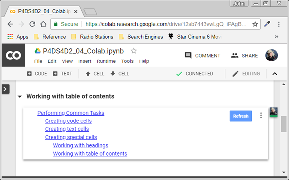
FIGURE 4-12: Adding a table of contents to your notebook makes the information more accessible.
The Table of Contents cell contains a heading in the actual cell that you can modify in the same way as any other heading in your notebook. The table of contents appears in the cell output. To update the table of contents, click Refresh to the right of the cell output. You also have access to all the usual text cell features when working with a Table of Contents cell.
The table of contents feature does appear in Notebook, but it’s not usable. If you plan to share the notebook with people who use Notebook, you should remove the table of contents to avoid potential confusion.
Editing cells
Both Colab and Notebook have Edit menus that contain the options you except, such as the ability to cut, copy, and paste cells. The two products have some interesting differences. For example, Notebook allows you to split and merge cells. Colab contains an option to show or hide the code as a toggle. These differences give each product a slightly different flavor but don’t really change your ability to use it to create and modify Python code.
Moving cells
The same technique you use for moving cells in Notebook also works with Colab. The only difference is that Colab relies exclusively on toolbar buttons, while Notebook also has cell movement options on the Edit menu.
Using Hardware Acceleration
Your Colab code executes on a Google server. All your computing device does is host a browser that displays the code and its results. Consequently, any special hardware on your computing device is ignored unless you choose to execute code locally.
Fortunately, you do have another option when working with Colab. Choose Edit ⇒ Notebook Settings to display the Notebook Settings dialog box shown in Figure 4-13. This dialog box lets you choose the Python runtime and gives you a way to add GPU execution for your code. The article at https://medium.com/deep-learning-turkey/google-colab-free-gpu-tutorial-e113627b9f5d provides additional details on how this feature works. The availability of a GPU isn’t an invitation to run large computations using Colab. The content at https://research.google.com/colaboratory/faq.html#gpu-availability tells you about the limitations of the Colab hardware acceleration (including that it may not be available when you need it).
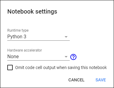
FIGURE 4-13: Hardware acceleration speeds code execution.
The Notebook Settings dialog box also lets you choose whether to include cell output when saving the notebook. Given that you store your notebook in the cloud in most cases and that loading large files into your browser can be time consuming, this feature enables you to restart a session more quickly. Of course, the trade-off is that you must now regenerate all the outputs you need.
Executing the Code
For your to be useful, you need to run it at some point. Previous sections have mentioned the right-pointing arrow that appears in the current cell. Clicking it runs just the current cell. Of course, you have other options than clicking the right-pointing arrow, and all these options appear on the Runtime menu. The following list summarizes these options:
- Running the current cell: Besides clicking the right-pointing arrow, you can also choose Runtime ⇒ Run the Focused Cell to execute the code in the current cell.
- Running other cells: Colab provides options on the Runtime menu for executing the code in the next cell, the previous cell, or a selection of cells. Simply choose the option that matches the cell or set of cells you want to execute.
- Running all the cells: In some cases, you want to execute all the code in a notebook. In this case, choose Runtime ⇒ Run All. Execution starts at the top of the notebook, in the first cell containing code, and continues to the last cell that contains code in the notebook. You can stop execution at any time by choosing Runtime ⇒ Interrupt Execution.
Choosing Runtime ⇒ Manage Sessions displays a dialog box containing a list of all the sessions that are currently executing for your account on Colab. You can use this dialog box to determine when the code in that notebook last executed and how much memory the notebook consumes. Click Terminate to end execution for a particular notebook. Click Close to close the dialog box and return to your current notebook.
Viewing Your Notebook
A notebook has a right-pointing arrow in its left margin. Clicking this icon displays a pane containing tabs that show various kinds of information about your notebook. You can also choose specific pieces of information to see from the View menu. To close this pane, click the X in the upper-right corner of the pane. The following sections describe each of these pieces of information.
Displaying the table of contents
Choose View ⇒ Table of Contents to see a table of contents for your notebook, as shown in Figure 4-14. Clicking any of the entries takes you to that section of the notebook.

FIGURE 4-14: Use the table of contents to navigate your notebook.
At the bottom of the pane is a + Section button. Click this button to create a new header cell below the currently selected cell.
Getting notebook information
When you choose View ⇒ Notebook Information, you see a pane open at the bottom of the browser, as shown in Figure 4-15. This pane contains the notebook size, settings, and owner. Notice that the display also tells you the maximum notebook size.
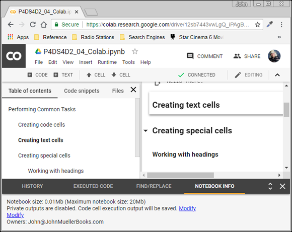
FIGURE 4-15: The notebook information includes both size and settings.
The Notebook Info tab also includes a Modify link (two of them). Both links display the Notebook Settings dialog box, in which you can choose the runtime type and whether the notebook relies on hardware acceleration, as described in the “Using Hardware Acceleration” section, earlier in this chapter.
Checking code execution
Colab keeps track of your code as you execute it. Choose View ⇒ Executed Code History to display the Executed Code tab in the pane at the bottom of the window, as shown in Figure 4-16. Note that the number associated with the entries in the Executed Code tab may not match the numbers associated with the associated cells. In addition, each unique execution of code receives a separate number.

FIGURE 4-16: Colab tracks which code you execute and in what order.
Sharing Your Notebook
You can share your Colab notebooks in a number of ways. For example, you can save it to GitHub or GitHub Gists. However, the two most direct methods are the following:
- Create a share message and send it to the recipient.
- Obtain a link to the code and send the link to the recipient.
In both cases, you click the Share button in the upper right of the Colab window. The Share with Others dialog box opens (see Figure 4-17).

FIGURE 4-17: Send a message or obtain a link to share your notebook.
When you enter one or more names in the People field, an additional field opens in which to add a sharing message. You can type a message and click Send to send the link immediately. If you click Advanced instead, you see another dialog box, where you can define how to share the notebook.
In the upper-right corner of the Share with Others dialog box, you see the Get Shareable Link button. Click this button to display a dialog box containing the link for your notebook. Clicking Copy Link places the URL on the Clipboard for your device, and you can paste it into messages or other forms of communication with others.
Getting Help
The most obvious place to obtain help with Colab is from the Colab Help menu. This menu contains all the usual entries for accessing frequently asked questions (FAQs) pages. The menu doesn’t have a link to general help, but you can find general help at https://colab.research.google.com/notebooks/welcome.ipynb (which requires you to log into the Colab site). The menu also provides options for submitting a bug and sending feedback.
One of the more intriguing Help menu entries is Search Code Snippets. This option opens the pane shown in Figure 4-18, in which you can search for example code that could meet your needs with a little modification. Clicking the Insert button inserts the code at the current cursor location in the cell that has focus. Each of the entries also shows an example of the code.
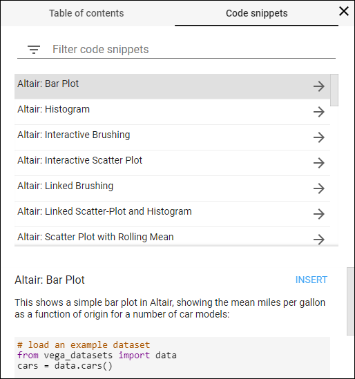
FIGURE 4-18: Use code snippets to write your applications more quickly.
Colab enjoys strong community support. Choosing Help ⇒ Ask a Question on Stack Overflow displays a new browser tab, where you can ask questions from other users. You see a login screen if you haven’t already logged into Stack Overflow.