
Chapter 3
Setting Up Python for Data Science
IN THIS CHAPTER
![]() Obtaining an off-the-shelf solution
Obtaining an off-the-shelf solution
![]() Creating an Anaconda installation on Linux, Mac OS, and Windows
Creating an Anaconda installation on Linux, Mac OS, and Windows
![]() Getting and installing the datasets and example code
Getting and installing the datasets and example code
Before you can do too much with Python or use it to solve data science problems, you need a workable installation. In addition, you need access to the datasets and code used for this book. Downloading the sample code and installing it on your system is the best way to get a good learning experience from the book. This chapter helps you get your system set up so that you can easily follow the examples in the remainder of the book.
This book relies on Jupyter Notebook version 5.5.0 supplied with the Anaconda 3 environment (version 5.2.0) that supports the Python version 3.6.5 to create the coding examples. For the examples to work, you must use Python 3.6.5 and the packages’ version as present in the Anaconda 3 version 5.2.0. Older versions of both Python and its packages tend to lack needed features, and newer versions tend to produce breaking changes. If you use some other version of Python, the examples are likely not going to work as intended. However, you can find other development tools that you may prefer to Jupyter Notebook. As part of looking at tools that you can use to write Python code, this chapter also reviews a few other offerings. If you choose one of these other offerings, your screenshots won’t match those provided in the book and you won’t be able to following the procedures, but if the package you choose supports Python 3.6.5, the code should still run as described in the book.
 Using the downloadable source doesn’t prevent you from typing the examples on your own, following them using a debugger, expanding them, or working with the code in all sorts of ways. The downloadable source is there to help you get a good start with your data science and Python learning experience. After you see how the code works when it’s correctly typed and configured, you can try to create the examples on your own. If you make a mistake, you can compare what you’ve typed with the downloadable source and discover precisely where the error exists. You can find the downloadable source for this chapter in the
 P4DS4D2_03_Sample.ipynb and P4DS4D2_03_Dataset_Load.ipynb files. (The Introduction tells you where to download the source code for this book.)
Considering the Off-the-Shelf Cross-Platform Scientific Distributions
It’s entirely possible to obtain a generic copy of Python and add all of the required data science libraries to it. The process can be difficult because you need to ensure that you have all the required libraries in the correct versions to ensure success. In addition, you need to perform the configuration required to ensure that the libraries are accessible when you need them. Fortunately, going through the required work is not necessary because a number of Python data science products are available for you to use. These products provide everything needed to get started with data science projects.
You can use any of the packages mentioned in the following sections to work with the examples in this book. However, the book’s source code and downloadable source rely on Continuum Analytics Anaconda because this particular package works on every platform this book is designed to support: Linux, Mac OS X, and Windows. The book doesn’t mention a specific package in the chapters that follow, but any screenshots reflect how things look when using Anaconda on Windows. You may need to tweak the code to use another package, and the screens will look different if you use Anaconda on some other platform.
Getting Continuum Analytics Anaconda
The basic Anaconda package is a free download that you obtain at https://www.anaconda.com/download/ (you may need to go to https://repo.anaconda.com/archive/ to obtain the 5.2.0 version used in this book if a newer version of the product is available when you visit the main site). Simply click one of the Python 3.6 Version links to obtain access to the free product. The filename you want begins with Anaconda3-5.2.0- followed by the platform and 32-bit or 64-bit version, such as Anaconda3-5.2.0-Windows-x86_64.exe for the Windows 64-bit version. Anaconda supports the following platforms:
- Windows 32-bit and 64-bit (the installer may offer you only the 64-bit or 32-bit version, depending on which version of Windows it detects)
- Linux 32-bit and 64-bit
- Mac OS X 64-bit
The default download version installed Python 3.6, which is the version used in this book. You can also choose to install Python 2.7 by clicking one of the Python 2.7 Version links. Both Windows and Mac OS X provide graphical installers. When using Linux, you rely on the bash utility.
 Obtaining Anaconda with older versions of Python is possible. If you want to use an older version of Python, click the installer archive link about halfway down the page. You should use only an older version of Python when you have a pressing need to do so.
The free product is all you need for this book. However, when you look on the site, you see that many other add-on products are available. These products can help you create robust applications. For example, when you add Accelerate to the mix, you obtain the ability to perform multicore and GPU-enabled operations. The use of these add-on products is outside the scope of this book, but the Anaconda site provides details on using them.
Getting Enthought Canopy Express
Enthought Canopy Express is a free product for producing both technical and scientific applications using Python. You can obtain it at https://www.enthought.com/canopy-express/. Click Download on the main page to see a listing of the versions that you can download. Only Canopy Express is free, the full Canopy product comes at a cost. Canopy Express supports the following platforms:
- Windows 32-bit and 64-bit
- Linux 32-bit and 64-bit
- Mac OS X 32-bit and 64-bit
 As of this writing, Canopy supports Python 3.5. You need Python 3.6 to ensure that the examples will run as anticipated. Make sure to download a version of Canopy that provides Python 3.6 support or be aware that some examples in the book may not work. The page at
 https://www.enthought.com/product/canopy/#/package-index lists packages that work with Python 3.6.
Choose the platform and version you want to download. When you click Download Canopy Express, you see an optional form for providing information about yourself. The download starts automatically, even if you don’t provide personal information to the company.
One of the advantages of Canopy Express is that Enthought is heavily involved in providing support for both students and teachers. People also can take classes, including online classes, that teach the use of Canopy Express in various ways (see https://training.enthought.com/courses). Also offered is live classroom training specifically designed for the data scientist; read about this training at https://www.enthought.com/services/training/data-science.
Getting WinPython
The name tells you that WinPython is a Windows-only product, which you can find at http://winpython.github.io/. That site provides Python 3.5, 3.6 and 3.7 support. This product is actually a takeoff of Python(x,y) (an IDE that went dormant in 2015 and stopped being developed; see http://python-xy.github.io/) and isn’t simply meant to replace it. Quite the contrary: WinPython gives you a more flexible way to work with Python(x,y). You can read about the initial motivation for creating WinPython at http://sourceforge.net/p/winpython/wiki/Roadmap/ and about its most recent development roadmap at https://github.com/winpython/winpython/wiki/Roadmap.
The bottom line for this product is that you gain flexibility at the cost of friendliness and a little platform integration. However, for developers who need to maintain multiple versions of an IDE, WinPython may make a significant difference. When using WinPython with this book, make sure to pay particular attention to configuration issues or you’ll find that even the downloadable code has little chance of working.
Installing Anaconda on Windows
Anaconda comes with a graphical installation application for Windows, so getting a good install means using a wizard, much as you would for any other installation. Of course, you need a copy of the installation file before you begin, and you can find the required download information in the “Getting Continuum Analytics Anaconda” section of this chapter. The following procedure should work fine on any Windows system, whether you use the 32-bit or the 64-bit version of Anaconda.
Locate the downloaded copy of Anaconda on your system.
The name of this file varies, but normally it appears as
Anaconda3-5.2.0-Windows-x86.exefor 32-bit systems andAnaconda3-5.2.0-Windows-x86_64.exefor 64-bit systems. The version number is embedded as part of the filename. In this case, the filename refers to version 5.2.0, which is the version used for this book. If you use some other version, you may experience problems with the source code and need to make adjustments when working with it.Double-click the installation file.
(You may see an Open File – Security Warning dialog box that asks whether you want to run this file. Click Run if you see this dialog box pop up.) You see an Anaconda 5.2.0 Setup dialog box similar to the one shown in Figure 3-1. The exact dialog box you see depends on which version of the Anaconda installation program you download. If you have a 64-bit operating system, it’s always best to use the 64-bit version of Anaconda so that you obtain the best possible performance. This first dialog box tells you when you have the 64-bit version of the product.
Click Next.
The wizard displays a licensing agreement. Be sure to read through the licensing agreement so that you know the terms of usage.
Click I Agree if you agree to the licensing agreement.
You’re asked what sort of installation type to perform, as shown in Figure 3-2. In most cases, you want to install the product just for yourself. The exception is if you have multiple people using your system and they all need access to Anaconda.
Choose one of the installation types and then click Next.
The wizard asks where to install Anaconda on disk, as shown in Figure 3-3. The book assumes that you use the default location. If you choose some other location, you may have to modify some procedures later in the book to work with your setup.
Choose an installation location (if necessary) and then click Next.
You see the Advanced Installation Options, shown in Figure 3-4. These options are selected by default and there isn’t a good reason to change them in most cases. You might need to change them if Anaconda won’t provide your default Python 3.6 setup. However, the book assumes that you’ve set up Anaconda using the default options.
The Add Anaconda to My PATH Environment Variable option is cleared by default, and you should leave it cleared. Adding it to the PATH environment variable does offer the ability to locate the Anaconda files when using a standard command prompt, but if you have multiple versions of Anaconda installed, only the first version you installed is accessible. Opening an Anaconda Prompt instead is far better so that you gain access to the version you expect.Change the advanced installation options (if necessary) and then click Install.
You see an Installing dialog box with a progress bar. The installation process can take a few minutes, so get yourself a cup of coffee and read the comics for a while. When the installation process is over, you see a Next button enabled.
Click Next.
The wizard tells you that the installation is complete.
Click Next.
Anaconda offers you the chance to integrate Visual Studio code support. You don’t need this support for this book, and adding it could potentially change the way that the Anaconda tools work. Unless you absolutely need Visual Studio support, you want to keep the Anaconda environment pure.
Click Skip.
You see a completion screen. This screen contains options to discover more about Anaconda Cloud and obtain information about starting your first Anaconda project. Selecting these options (or clearing them) depends on what you want to do next; the options don’t affect your Anaconda setup.
Select any required options. Click Finish.
You’re ready to begin using Anaconda.

FIGURE 3-1: The setup process begins by telling you whether you have the 64-bit version.
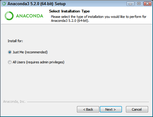
FIGURE 3-2: Tell the wizard how to install Anaconda on your system.
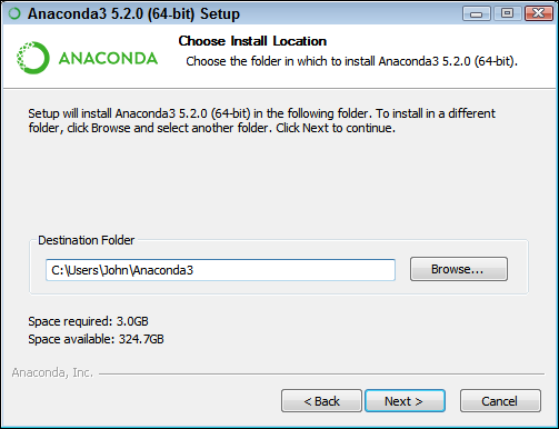
FIGURE 3-3: Specify an installation location.
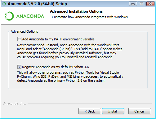
FIGURE 3-4: Configure the advanced installation options.
Installing Anaconda on Linux
You use the command line to install Anaconda on Linux — there is no graphical installation option. Before you can perform the install, you must download a copy of the Linux software from the Continuum Analytics site. You can find the required download information in the “Getting Continuum Analytics Anaconda” section of this chapter. The following procedure should work fine on any Linux system, whether you use the 32-bit or the 64-bit version of Anaconda.
Open a copy of Terminal.
You see the Terminal window appear.
Change directories to the downloaded copy of Anaconda on your system.
The name of this file varies, but normally it appears as
Anaconda3-5.2.0-Linux-x86.shfor 32-bit systems andAnaconda3-5.2.0-Linux-x86_64.shfor 64-bit systems. The version number is embedded as part of the filename. In this case, the filename refers to version 5.2.0, which is the version used for this book. If you use some other version, you may experience problems with the source code and need to make adjustments when working with it.Type bash Anaconda3-5.2.0-Linux-x86 (for the 32-bit version) or Anaconda3-5.2.0-Linux-x86_64.sh (for the 64-bit version) and press Enter.
An installation wizard starts that asks you to accept the licensing terms for using Anaconda.
Read the licensing agreement and accept the terms using the method required for your version of Linux.
The wizard asks you to provide an installation location for Anaconda. The book assumes that you use the default location of ~/anaconda. If you choose some other location, you may have to modify some procedures later in the book to work with your setup.
Provide an installation location (if necessary) and press Enter (or click Next).
You see the application extraction process begin. After the extraction is complete, you see a completion message.
Add the installation path to your
PATHstatement using the method required for your version of Linux.You’re ready to begin using Anaconda.
Installing Anaconda on Mac OS X
The Mac OS X installation comes only in one form: 64-bit. Before you can perform the install, you must download a copy of the Mac software from the Continuum Analytics site. You can find the required download information in the “Getting Continuum Analytics Anaconda” section of this chapter. The following steps help you install Anaconda 64-bit on a Mac system.
Locate the downloaded copy of Anaconda on your system.
The name of this file varies, but normally it appears as
Anaconda3-5.2.0-MacOSX-x86_64.pkg. The version number is embedded as part of the filename. In this case, the filename refers to version 5.2.0, which is the version used for this book. If you use some other version, you may experience problems with the source code and need to make adjustments when working with it.Double-click the installation file.
You see an introduction dialog box.
Click Continue.
The wizard asks whether you want to review the Read Me materials. You can read these materials later. For now, you can safely skip the information.
Click Continue.
The wizard displays a licensing agreement. Be sure to read through the licensing agreement so that you know the terms of usage.
Click I Agree if you agree to the licensing agreement.
The wizard asks you to provide a destination for the installation. The destination controls whether the installation is for an individual user or a group.
You may see an error message stating that you can’t install Anaconda on the system. The error message occurs because of a bug in the installer and has nothing to do with your system. To get rid of the error message, choose the Install Only for Me option. You can’t install Anaconda for a group of users on a Mac system.Click Continue.
The installer displays a dialog box containing options for changing the installation type. Click Change Install Location if you want to modify where Anaconda is installed on your system (the book assumes that you use the default path of ~/anaconda). Click Customize if you want to modify how the installer works. For example, you can choose not to add Anaconda to your
PATHstatement. However, the book assumes that you have chosen the default install options and there isn’t a good reason to change them unless you have another copy of Python 2.7 installed somewhere else.Click Install.
You see the installation begin. A progress bar tells you how the installation process is progressing. When the installation is complete, you see a completion dialog box.
Click Continue.
You’re ready to begin using Anaconda.
Downloading the Datasets and Example Code
This book is about using Python to perform data science tasks. Of course, you could spend all your time creating the example code from scratch, debugging it, and only then discovering how it relates to data science, or you can take the easy way and download the prewritten code so that you can get right to work. Likewise, creating datasets large enough for data science purposes would take quite a while. Fortunately, you can access standardized, precreated datasets quite easily using features provided in some of the data science libraries. The following sections help you download and use the example code and datasets so that you can save time and get right to work with data science–specific tasks.
Using Jupyter Notebook
To make working with the relatively complex code in this book easier, you use Jupyter Notebook. This interface makes it easy to create Python notebook files that can contain any number of examples, each of which can run individually. The program runs in your browser, so which platform you use for development doesn’t matter; as long as it has a browser, you should be OK.
Starting Jupyter Notebook
Most platforms provide an icon to access Jupyter Notebook. All you need to do is open this icon to access Jupyter Notebook. For example, on a Windows system, you choose Start ⇒ All Programs ⇒ Anaconda3 ⇒ Jupyter Notebook. Figure 3-5 shows how the interface looks when viewed in a Firefox browser. The precise appearance on your system depends on the browser you use and the kind of platform you have installed.

FIGURE 3-5: Jupyter Notebook provides an easy method to create data science examples.
If you have a platform that doesn’t offer easy access through an icon, you can use these steps to access Jupyter Notebook:
Open an Anaconda Prompt, Command Prompt, or Terminal Window on your system.
You see the window open so that you can type commands.
Change directories to the
Anaconda3Scriptsdirectory on your machine.Most systems let you use the
CDcommand for this task.Type ..python Jupyter-script.py notebook and press Enter.
The Jupyter Notebook page opens in your browser.
Stopping the Jupyter Notebook server
No matter how you start Jupyter Notebook (or just Notebook, as it appears in the remainder of the book), the system generally opens a command prompt or terminal window to host Notebook. This window contains a server that makes the application work. After you close the browser window when a session is complete, select the server window and press Ctrl+C or Ctrl+Break to stop the server.
Defining the code repository
The code you create and use in this book will reside in a repository on your hard drive. Think of a repository as a kind of filing cabinet where you put your code. Notebook opens a drawer, takes out the folder, and shows the code to you. You can modify it, run individual examples within the folder, add new examples, and simply interact with your code in a natural manner. The following sections get you started with Notebook so that you can see how this whole repository concept works.
Defining a new folder
You use folders to hold your code files for a particular project. The project for this book is P4DS4D2 (which stands for Python for Data Science For Dummies, 2nd Edition). The following steps help you create a new folder for this book.
Choose New ⇒ Folder.
Notebook creates a new folder for you. The name of the folder can vary, but for Windows users, it’s simply listed as Untitled Folder. You may have to scroll down the list of available folders to find the folder in question.
- Place a check in the box next to Untitled Folder.
Click Rename at the top of the page.
You see the Rename Directory dialog box, shown in Figure 3-6.
Type P4DS4D2 and press Enter.
Notebook renames the folder for you.

FIGURE 3-6: Create a folder to use to hold the book’s code.
Creating a new notebook
Every new notebook is like a file folder. You can place individual examples within the file folder, just as you would sheets of paper into a physical file folder. Each example appears in a cell. You can put other sorts of things in the file folder, too, but you see how these things work as the book progresses. Use these steps to create a new notebook.
Click the P4DS4D2 entry on the Home page.
You see the contents of the project folder for this book, which will be blank if you’re performing this exercise from scratch.
Choose New ⇒ Python 3.
You see a new tab open in the browser with the new notebook, as shown in Figure 3-7. Notice that the notebook contains a cell and that Notebook has highlighted the cell so that you can begin typing code in it. The title of the notebook is Untitled right now. That’s not a particularly helpful title, so you need to change it.
Click Untitled on the page.
Notebook asks whether you want to use a new name, as shown in Figure 3-8.
Type P4DS4D2_03_Sample and press Enter.
The new name tells you that this is a file for Python for Data Science For Dummies, 2nd Edition, Chapter 3, Sample.ipynb. Using this naming convention will let you easily differentiate these files from other files in your repository.

FIGURE 3-7: A notebook contains cells that you use to hold code.

FIGURE 3-8: Provide a new name for your notebook.
Adding notebook content
Of course, the Sample notebook doesn’t contain anything just yet. This book follows a convention of putting the source code files together that makes them easy to use. The following steps tell you about this convention:
Choose Markdown from the drop-down list that currently contains the word Code.
A Markdown cell contains documentation text. You can put anything in a Markdown cell because Notebook won’t interpret it. By using Markdown cells, you can easily document precisely what you mean when writing code.
Type # Downloading the Datasets and Example Code and click Run (the button with the right-pointing arrow on the toolbar).
The hash mark (#) creates a heading. A single # creates a first-level heading. The text that follows contains that actual heading information. Clicking Run turns the formatted text into a heading, as shown in Figure 3-9. Notice that Notebook automatically creates a new cell for you to use.
Choose Markdown, type ## Defining the code repository, and click Run.
Notebook creates a second-level heading, which looks smaller than a first-level heading.
Choose Markdown, type ### Adding notebook content, and click Run.
Notebook creates a third-level heading. Your headings now match the hierarchy that starts with the first-level heading for this section. Using this approach helps you to easily locate a particular piece of code in the downloadable source. As always, Notebook creates a new cell for you, and the cell type automatically changes to Code, so you’re ready to type some code for this example.
Type print(’Python is really cool!’) and click Run.
Notice that the code is color coded so that you can tell the different between a function (
print) and its associated data (’Python is really cool!’). You see the output shown in Figure 3-10. The output is part of the same cell as the code. However, Notebook visually separates the output from the code so that you can tell them apart. Notebook automatically creates a new cell for you.

FIGURE 3-9: Create headings to document your code.

FIGURE 3-10: Notebook uses cells to store your code.
When you finish working with a notebook, shutting it down is important. To close a notebook, choose File ⇒ Close and Halt. You return to the P4DS4D2 page, where you can see the notebook you just created added to the list, as shown in Figure 3-11.

FIGURE 3-11: Any notebooks you create appear in the repository list.
Exporting a notebook
It isn’t much fun to create notebooks and keep them all to yourself. At some point, you want to share them with other people. To perform this task, you must export your notebook from the repository to a file. You can then send the file to someone else who will import it into his or her repository.
The previous section shows how to create a notebook named P4DS4D2_03_Sample. You can open this notebook by clicking its entry in the repository list. The file reopens so that you can see your code again. To export this code, choose File ⇒ Download As ⇒ Notebook (.ipynb). What you see next depends on your browser, but you generally see some sort of dialog box for saving the notebook as a file. Use the same method for saving the Notebook file as you use for any other file you save using your browser.
Removing a notebook
Sometimes notebooks get outdated or you simply don’t need to work with them any longer. Rather than allow your repository to get clogged with files you don’t need, you can remove these unwanted notebooks from the list. Notice the check box next to the P4DS4D2_03_Sample.ipynb entry in Figure 3-11. Use these steps to remove the file:
- Select the check box next to the
P4DS4D2_03_Sample.ipynbentry. Click the Delete (trashcan) icon.
You see a Delete notebook warning message like the one shown in Figure 3-12.
Click Delete.
Notebook removes the notebook file from the list.
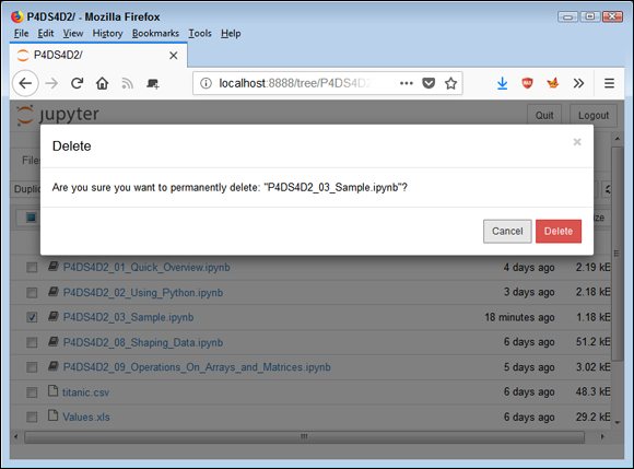
FIGURE 3-12: Notebook warns you before removing any files from the repository.
Importing a notebook
To use the source code from this book, you must import the downloaded files into your repository. The source code comes in an archive file that you extract to a location on your hard drive. The archive contains a list of .ipynb (IPython Notebook) files containing the source code for this book (see the Introduction for details on downloading the source code). The following steps tell how to import these files into your repository:
Click Upload on the Notebook P4DS4D2 page.
What you see depends on your browser. In most cases, you see some type of File Upload dialog box that provides access to the files on your hard drive.
- Navigate to the directory containing the files you want to import into Notebook.
Highlight one or more files to import and click the Open (or other, similar) button to begin the upload process.
You see the file added to an upload list, as shown in Figure 3-13. The file isn’t part of the repository yet — you’ve simply selected it for upload.
Click Upload.
Notebook places the file in the repository so that you can begin using it.
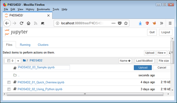
FIGURE 3-13: The files you want to add to the repository appear as part of an upload list.
Understanding the datasets used in this book
This book uses a number of datasets, all of which appear in the Scikit-learn library. These datasets demonstrate various ways in which you can interact with data, and you use them in the examples to perform a variety of tasks. The following list provides a quick overview of the function used to import each of the datasets into your Python code:
load_boston(): Regression analysis with the Boston house-prices datasetload_iris(): Classification with the Iris datasetload_diabetes(): Regression with the diabetes datasetload_digits([n_class]): Classification with the digits datasetfetch_20newsgroups(subset=’train’):Data from 20 newsgroupsfetch_olivetti_faces(): Olivetti faces dataset from AT&T
The technique for loading each of these datasets is the same across examples. The following example shows how to load the Boston house-prices dataset. You can find the code in the P4DS4D2_03_Dataset_Load.ipynb notebook.
from sklearn.datasets import load_boston
Boston = load_boston()
print(Boston.data.shape)
To see how the code works, click Run Cell. The output from the print call is (506L, 13L). You can see the output shown in Figure 3-14. (Be patient; the dataset load can require a few seconds to complete.)

FIGURE 3-14: The Boston object contains the loaded dataset.