
Chapter 18
Performing Cross-Validation, Selection, and Optimization
IN THIS CHAPTER
![]() Learning about overfitting and underfitting
Learning about overfitting and underfitting
![]() Choosing the right metric to monitor
Choosing the right metric to monitor
![]() Cross-validating the results
Cross-validating the results
![]() Selecting the best features for machine learning
Selecting the best features for machine learning
![]() Optimizing hyperparameters
Optimizing hyperparameters
Machine learning algorithms can indeed learn from data. For instance, the four algorithms presented in the previous chapter, although quite simple, can effectively estimate a class or a value after being presented with examples associated with outcomes. It is all a matter of learning by induction, which is the process of extracting general rules from specific examples. From childhood, humans commonly learn by seeing examples, deriving some general rules or ideas from them, and then successfully applying the derived rule to new situations as we grow up. For example, if we see someone being burned after touching fire, we understand that fire is dangerous, and we don’t need to touch it ourselves to know that.
Learning by example using machine algorithms has pitfalls. Here are a few issues that might arise:
- There aren’t enough examples to make a judgment about a rule, no matter what machine learning algorithm you are using.
- The machine learning application is presented with the wrong examples and consequently cannot reason correctly.
- Even when the application sees enough right examples, it still can’t figure out rules because they’re too complex. Sir Isaac Newton, the father of modern physics, narrated the story that he was inspired by the fall of an apple from a tree in his formulation of gravity. Unfortunately, deriving a universal law from a series of observations is not an automatic consequence for most of us and the same applies to algorithms.
It’s important to consider these pitfalls when delving into machine learning. The quantity of data, its quality, and the characteristics of the learning algorithm decide whether a machine learning application can generalize well to new cases. If anything is wrong with any of them, they can pose some serious limits. As a data science practitioner, you must recognize and learn to avoid these types of pitfalls in your data science experiments.
 You don’t have to type the source code for this chapter manually. In fact, it’s a lot easier if you use the downloadable source (see the Introduction for download instructions). The source code for this chapter appears in the
 P4DS4D2_18_Performing_Cross_Validation_Selection_and_Optimization.ipynb source code file.
Pondering the Problem of Fitting a Model
Fitting a model implies learning from data a representation of the rules that generated the data in the first place. From a mathematical perspective, fitting a model is analogous to guessing an unknown function of the kind you faced in high school, such as, y=4x^2+2x, just by observing its y results. Therefore, under the hood, you expect that machine learning algorithms generate mathematical formulations by determining how reality works based on the examples provided.
Demonstrating whether such formulations are real is beyond the scope of data science. What is most important is that they work by producing exact predictions. For example, even though you can describe much of the physical world using mathematical functions, you often can’t describe social and economic dynamics this way — but people try guessing them anyway.
To summarize, as a data scientist, you should always strive to approximate the real, unknown functions underlying the problems you face using the best information available. The result of your work is evaluated based on your capacity to predict specific outcomes (the target outcome) given certain premises (the data) thanks to a useful range of algorithms (the machine learning algorithms).
Earlier in the book, you see something akin to a real function or law when the book presents linear regression, which has its own formulation. The linear formula y = Bx + a, which mathematically represents a line on a plane, can often approximate training data well, even if the data is not representing a line or something similar to a line. As with linear regression, all other machine learning algorithms have an internal formulation themselves (and some, such as neural networks, even require you to define their formulation from scratch). The linear regression’s formulation is one of the simplest ones; formulations from other learning algorithms can appear quite complex. You don’t need to know exactly how they work. You do need to have an idea of how complex they are, whether they represent a line or a curve, and whether they can sense outliers or noisy data. When planning to learn from data, you should address these problematic aspects based on the formulation you intend to use:
- Whether the learning algorithm is the best one that can approximate the unknown function that you imagine behind the data you are using. In order to make such a decision, you must consider the learning algorithm’s formulation performance on the data at hand and compare it with other, alternative formulations from other algorithms.
- Whether the specific formulation of the learning algorithm is too simple, with respect to the hidden function, to make an estimate (this is called a bias problem).
- Whether the specific formulation of the learning algorithm is too complex, with respect to the hidden function to be guessed (leading to the variance problem).
Not all algorithms are suitable for every data problem. If you don’t have enough data or the data is full of erroneous information, it may be too difficult for some formulations to figure out the real function.
Understanding bias and variance
If your chosen learning algorithm can’t learn properly from data and is not performing well, the cause is bias or variance in its estimates.
- Bias: Given the simplicity of formulation, your algorithm tends to overestimate or underestimate the real rules behind the data and is systematically wrong in certain situations. Simple algorithms have high bias; having few internal parameters, they tend to represent only simple formulations well.
- Variance: Given the complexity of formulation, your algorithm tends to learn too much information from the data and detect rules that don’t exist, which causes its predictions to be erratic when faced with new data. You can think of variance as a problem connected to memorization. Complex algorithms can memorize data features thanks to the algorithms’ high number of internal parameters. However, memorization doesn’t imply any understanding about the rules.
Bias and variance depend on the complexity of the formulation at the core of the learning algorithm with respect to the complexity of the formulation that is presumed to have generated the data you are observing. However, when you consider a specific problem using the available data rules, you’re better off having high bias or variance when
- You have few observations: Simpler algorithms perform better, no matter what the unknown function is. Complex algorithms tend to learn too much from data, estimating with inaccuracy.
- You have many observations: Complex algorithms always reduce variance. The reduction occurs because even complex algorithms can’t learn all that much from data, so they learn just the rules, not any erratic noise.
- You have many variables: Provided that you also have many observations, simpler algorithms tend to find a way to approximate even complex hidden functions.
Defining a strategy for picking models
When faced with a machine learning problem, you usually know little about the problem and don’t know whether a particular algorithm will manage it well. Consequently, you don’t really know whether the source of a problem is caused by bias or variance — although you can usually use the rule of thumb that if an algorithm is simple, it will have high bias, and if it is complex, it will have high variance. Even when working with common, well-documented data science applications, you’ll notice that what works in other situations (as described in academic and industry papers) often doesn’t operate very well for your own application because the data is different.
You can summarize this situation using the famous no-free-lunch theorem of the mathematician David Wolpert: Any two machine learning algorithms are equivalent in performance when tested across all possible problems. Consequently, it isn’t possible to say that one algorithm is always better than another; it can be better than another one only when used to solve specific problems. You can view the concept in another way: For every problem, there is never a fixed recipe! The best and only strategy is just to try everything you can and verify the results using a controlled scientific experiment. Using this approach ensures that what seems to work is what really works and, most important, what will keep on working with new data. Although you may have more confidence when using some learners over others, you can never tell what machine learning algorithm is the best before trying it and measuring its performance on your problem.
At this point, you must consider a critical, yet underrated, aspect to ensure the success of your data project. For a best model and greatest results, it’s essential to define an evaluation metric that distinguishes a good model from a bad one with respect to the business or scientific problem that you want to solve. In fact, for some projects, you may need to avoid predicting negative cases when they are positive; for others, you may want to absolutely spot all the positive ones; and for still others, all you need to do is order them so that positive ones come before the negative ones and you don’t need to check them all.
By picking an algorithm, you automatically also pick an optimization process ruled by an evaluation metric that reports its performance to the algorithm so that the algorithm can better adjust its parameters. For instance, when using a linear regression, the metric is the mean squared error given by the vertical distance of the observations from the regression line. Therefore, it’s automatic, and you can more easily accept the algorithm performance provided by such a default evaluation metric.
Apart from accepting the default metric, some algorithms do let you choose a preferred evaluation function. In other cases, when you can’t point out a favorite evaluation function, you can still influence the existing evaluation metric by appropriately fixing some of its hyperparameters, thus optimizing the algorithm indirectly for another, different, metric.
Before starting to train your data and create predictions, always consider what could be the best performance measure for your project. Scikit-learn offers access to a wide range of measures for both classification and regression problems. The sklearn.metrics module allows you to call the optimization procedures using a simple string or by calling an error function from its modules. Table 18-1 shows the measures commonly used for regression problems.
TABLE 18-1 Regression Evaluation Measures
Callable String |
Function |
mean_absolute_error |
sklearn.metrics.mean_absolute_error |
mean_squared_error |
sklearn.metrics.mean_squared_error |
r2 |
sklearn.metrics.r2_score |
The r2 string specifies a statistical measure for linear regression called R2 (R squared). It expresses how the model compares in predictive power with respect to a simple mean. Machine learning applications seldom use this measure because it doesn’t explicitly report errors made by the model, although high R2 values imply fewer errors; more viable metrics for regression models are the mean squared errors and the mean absolute errors.
Squared errors penalize extreme values more, whereas absolute error weights all the errors the same. So it is really a matter of considering the trade-off between reducing the error on extreme observations as much as possible (squared error) or trying to reduce the error for the majority of the observations (absolute error). The choice you make depends on the application. When extreme values represent critical situations for your application, a squared error measure is better. However, when your concern is to minimize the common and usual observations, as often happens in forecasting sales problems, you should use a mean absolute error as the reference. The choices are even for complex classification problems, as you can see in Table 18-2.
TABLE 18-2 Classification Evaluation Measures
Callable String |
Function |
accuracy |
sklearn.metrics.accuracy_score |
precision |
sklearn.metrics.precision_score |
recall |
sklearn.metrics.recall_score |
f1 |
sklearn.metrics.f1_score |
roc_auc |
sklearn.metrics.roc_auc_score |
Accuracy is the simplest error measure in classification, counting (as a percentage) how many of the predictions are correct. It takes into account whether the machine learning algorithm has guessed the right class. This measure works with both binary and multiclass problems. Even though it’s a simple measure, optimizing accuracy may cause problems when an imbalance exists between classes. For example, it could be a problem when the class is frequent or preponderant, such as in fraud detection, where most transactions are actually legitimate with respect to a few criminal transactions. In such situations, machine learning algorithms optimized for accuracy tend to guess in favor of the preponderant class and be wrong most of time with the minor classes, which is an undesirable behavior for an algorithm that you expect to guess all the classes correctly, not just a few selected ones.
Precision and recall, and their conjoint optimization by F1 score, can solve problems not addressed by accuracy. Precision is about being precise when guessing. It tracks the percentage of times, when forecasting a class, that a class was right. For example, you can use precision when diagnosing cancer in patients after evaluating data about their exams. Your precision in this case is the percentage of patients who really have cancer among those diagnosed with cancer. Therefore, if you have diagnosed ten ill patients and nine are truly ill, your precision is 90 percent.
You face different consequences when you don’t diagnose cancer in a patient who has it or you do diagnose it in a healthy patient. Precision tells just a part of the story, because there are patients with cancer that you have diagnosed as healthy, and that’s a terrible problem. The recall measure tells the second part of the story. It reports, among an entire class, your percentage of correct guesses. For example, when reviewing the previous example, the recall metric is the percentage of patients that you correctly guessed have cancer. If there are 20 patients with cancer and you have diagnosed just 9 of them, your recall will be 45 percent.
When using your model, you can be accurate but still have low recall, or have a high recall but lose accuracy in the process. Fortunately, precision and recall can be maximized together using the F1 score, which uses the formula: F1 = 2 * (precision * recall) / (precision + recall). Using the F1 score ensures that you always get the best precision and recall combined.
Receiver Operating Characteristic Area Under Curve (ROC AUC) is useful when you want to order your classifications according to their probability of being correct. Therefore, when optimizing ROC AUC in the previous example, the learning algorithm will first try to order (sort) patients starting from those most likely to have cancer to those least likely to have cancer. The ROC AUC is higher when the ordering is good and low when it is bad. If your model has a high ROC AUC, you need to check the most likely ill patients. Another example is in a fraud detection problem, when you want to order customers according to the risk of being fraudulent. If your model has a good ROC AUC, you need to check just the riskiest customers closely.
Dividing between training and test sets
Having explored how to decide among the different error metrics for classification and regression, the next step in the strategy for choosing the best model is to experiment and evaluate the solutions by viewing their ability to generalize to new cases. As an example of correct procedures for experimenting with machine learning algorithms, begin by loading the Boston dataset (a popular example dataset created in the 1970s), which consists of Boston housing prices, various house characteristic measurements, and measures of the residential area where each house is located.
from sklearn.datasets import load_boston
boston = load_boston()
X, y = boston.data, boston.target
Notice that the dataset contains more than 500 observations and 13 features. The target is a price measure, so you decide to use linear regression and to optimize the result using the mean squared error. The objective is to ensure that a linear regression is a good model for the Boston dataset and to quantify how good it is using the mean squared error (which lets you compare it with alternative models).
from sklearn.linear_model import LinearRegression
from sklearn.metrics import mean_squared_error
regression = LinearRegression()
regression.fit(X,y)
print('Mean squared error: %.2f' % mean_squared_error(
y_true=y, y_pred=regression.predict(X)))
The resulting mean square error generated by the commands is
Mean squared error: 21.90
After having fitted the model with the data (which is called the training data because it provides examples to learn from), the mean_squared_error error function reports the data prediction error. The mean squared error is 21.90, apparently a good measure but calculated directly on the training set, so you cannot be sure if it could work as well with new data (machine learning algorithms are both good at learning and at memorizing from examples).
Ideally, you need to perform a test on data that the algorithm has never seen in order to exclude any memorization. Only in this way can you discover whether your algorithm will work well when new data arrives. To perform this task, you wait for new data, make the predictions on it, and then compare the predictions to reality. But, performing the task this way may take a long time and could become both risky and expensive, depending on the type of problem you want to solve using machine learning (for example, some applications such as cancer detection can be incredibly risky to experiment with because lives are at a stake).
Luckily, you have another way to obtain the same result. To simulate having new data, you can divide the observations into test and training cases. It’s quite common in data science to have a test size of 25–30 percent of the available data and to train the predictive model using the remaining 70–75 percent. Here is an example of how you can achieve data partitioning in Python:
from sklearn.model_selection import train_test_split
X_train, X_test, y_train, y_test = train_test_split(
X, y, test_size=0.30, random_state=5)
print(X_train.shape, X_test.shape)The code prints the resulting shapes of the training and test sets, with the former being 70 percent of the initial dataset size and the latter just 30 percent:
(354, 13) (152, 13)
The example separates training and test X and y variables into distinct variables using the train_test_split function. The test_size parameter indicates a test set made of 30 percent of the available observations. The function always chooses the test sample randomly. Now you can use the training set for training:
regression.fit(X_train,y_train)
print('Train mean squared error: %.2f' % mean_squared_error(
y_true=y_train, y_pred=regression.predict(X_train)))
The output shows the training set’s mean squared error:
Train mean squared error: 19.07
At this point, you fit the model again and the code reports a new training error of 19.07, which is somehow different from before. However, the error you really have to refer to comes from the test set you reserved.
print('Test mean squared error: %.2f' % mean_squared_error(
y_true=y_test, y_pred=regression.predict(X_test)))
After running the evaluation on the test set, you get its error value:
Test mean squared error: 30.70
When you the estimate the error on the test set, the results show that the reported value is 30.70. What a difference, indeed! Somehow, the estimate on the training set was too optimistic. Using the test set, while more realistic in error estimation, really makes your result depend on a small portion of the data. If you change that small portion, the test result will also change. Here is an example:
from sklearn.model_selection import train_test_split
X_train, X_test, y_train, y_test = train_test_split(
X, y, test_size=0.30, random_state=6)
regression.fit(X_train,y_train)
print('Train mean squared error: %.2f' % mean_squared_error(
y_true=y_train, y_pred=regression.predict(X_train)))
print('Test mean squared error: %.2f' % mean_squared_error(
y_true=y_test, y_pred=regression.predict(X_test)))
You get a new report of the errors in the train and test sets:
Train mean squared error: 19.48
Test mean squared error: 28.33
What you have experienced in this section is a common problem with machine learning algorithms. You know that each algorithm has a certain bias or variance in predicting an outcome; the problem is that you can’t estimate its impact for sure. Moreover, if you have to make choices with regard to the algorithm, you can’t be sure of which decision might be the most effective one.
Using training data is always unsuitable when evaluating algorithm performance because the learning algorithm can actually predict the training data better. This is especially true when an algorithm has a low bias because of its complexity. In this case, you can expect a lower error when predicting the training data, which means that you get an overly optimistic result that doesn’t compare it fairly with other algorithms (which may have a different bias/variance profile), nor are the results useful for this example’s evaluation. By using the test data, you actually reduce the training examples (which may cause the algorithm to perform less well), but in exchange, you get a more reliable and comparable error estimate.
Cross-Validating
If test sets provide unstable results because of sampling, the solution is to systematically sample a certain number of test sets and then average the results. It’s a statistical approach (to observe many results and take an average of them), and that’s the basis of cross-validation. The recipe is straightforward:
- Divide your data into folds (each fold is a container that holds an even distribution of the cases), usually 10, but fold sizes of 3, 5, and 20 are viable alternative options.
- Hold out one fold as a test set and use the others as training sets.
- Train and record the test set result. If you have little data, it’s better to use a larger number of folds, because the quantity of data and the use of additional folds positively affects the quality of training.
- Perform Steps 2 and 3 again, using each fold in turn as a test set.
- Calculate the average and the standard deviation of all the folds’ test results. The average is a reliable estimator of the quality of your predictor. The standard deviation will tell you the predictor reliability (if it is too high, the cross-validation error could be imprecise). Expect that predictors with high variance will have a high cross-validation standard deviation.
Even though this technique may appear complicated, Scikit-learn handles it using the functions in the sklearn.model_selection module.
Using cross-validation on k folds
To run cross-validation, you first have to initialize an iterator. KFold is the iterator that implements k folds cross-validation. There are other iterators available from the sklearn.model_selection module, mostly derived from the statistical practice, but KFold is the most widely used in data science practice.
KFold requires you to specify specify the n_splits number (the number of folds to generate), and indicate whether you want to shuffle the data (by using the shuffle parameter). As a rule, the higher the expected variance, the more that increasing the number of splits improves the mean estimate. It’s a good idea to shuffle the data because ordered data can introduce confusion into the learning processes for some algorithms if the first observations are different from the last ones.
After setting KFold, call the cross_val_score function, which returns an array of results containing a score (from the scoring function) for each cross-validation fold. You have to provide cross_val_score with your data (both X and y) as an input, your estimator (the regression class), and the previously instantiated KFold iterator (as the cv parameter). In a matter of a few seconds or minutes, depending on the number of folds and data processed, the function returns the results. You average these results to obtain a mean estimate, and you can also compute the standard deviation to check how stable the mean is.
from sklearn.model_selection import cross_val_score, KFold
import numpy as np
crossvalidation = KFold(n_splits=10, shuffle=True, random_state=1)
scores = cross_val_score(regression, X, y,
scoring='neg_mean_squared_error', cv=crossvalidation, n_jobs=1)
print('Folds: %i, mean squared error: %.2f std: %.2f' %
(len(scores),np.mean(np.abs(scores)),np.std(scores)))
Here is the result:
Folds: 10, mean squared error: 23.76 std: 12.13
 Cross-validating can work in parallel because no estimate depends on any other estimate. You can take advantage of the multiple cores present on your computer by setting the parameter
 n_jobs=-1.
Sampling stratifications for complex data
Cross-validation folds are decided by random sampling. Sometimes it may be necessary to track if and how much of a certain characteristic is present in the training and test folds in order to avoid malformed samples. For instance, the Boston dataset has a binary variable (a feature that has a value of 1 or 0) indicating whether the house bounds the Charles River. This information is important to understand the value of the house and determine whether people would like to spend more for it. You can see the effect of this variable using the following code.
%matplotlib inline
import pandas as pd
df = pd.DataFrame(X, columns=boston.feature_names)
df['target'] = y
df.boxplot('target', by='CHAS', return_type='axes');
A boxplot, represented in Figure 18-1, reveals that houses on the river tend to have values higher than other houses. Of course, there are expensive houses all around Boston, but you have to keep an eye about how many river houses you are analyzing because your model has to be general for all of Boston, not just Charles River houses.

FIGURE 18-1: Boxplot of the target outcome, grouped by CHAS.
In similar situations, when a characteristic is rare or influential, you can’t be sure when it’s present in the sample because the folds are created in a random way. Having too many or too few of a particular characteristic in each fold implies that the machine learning algorithm may derive incorrect rules.
The StratifiedKFold class provides a simple way to control the risk of building malformed samples during cross-validation procedures. It can control the sampling so that certain features, or even certain outcomes (when the target classes are extremely unbalanced), will always be present in your folds in the right proportion. You just need to point out the variable you want to control by using the y parameter, as shown in the following code.
from sklearn.model_selection import StratifiedShuffleSplit
from sklearn.metrics import mean_squared_error
strata = StratifiedShuffleSplit(n_splits=3,
test_size=0.35,
random_state=0)
scores = list()
for train_index, test_index in strata.split(X, X[:,3]):
X_train, X_test = X[train_index], X[test_index]
y_train, y_test = y[train_index], y[test_index]
regression.fit(X_train, y_train)
scores.append(mean_squared_error(y_true=y_test,
y_pred=regression.predict(X_test)))
print('%i folds cv mean squared error: %.2f std: %.2f' %
(len(scores),np.mean(np.abs(scores)),np.std(scores)))
The result from the 3-fold stratified cross-validation is
3 folds cv mean squared error: 24.30 std: 3.99
Although the validation error is similar, by controlling the CHAR variable, the standard error of the estimates decreases, making you aware that the variable was influencing the previous cross-validation results.
Selecting Variables Like a Pro
Selecting the right variables can improve the learning process by reducing the amount of noise (useless information) that can influence the learner’s estimates. Variable selection, therefore, can effectively reduce the variance of predictions. In order to involve just the useful variables in training and leave out the redundant ones, you can use these techniques:
- Univariate approach: Select the variables most related to the target outcome.
- Greedy or backward approach: Keep only the variables that you can remove from the learning process without damaging its performance.
Selecting by univariate measures
If you decide to select a variable by its level of association with its target, the class SelectPercentile provides an automatic procedure for keeping only a certain percentage of the best, associated features. The available metrics for association are
f_regression: Used only for numeric targets and based on linear regression performance.f_classif: Used only for categorical targets and based on the Analysis of Variance (ANOVA) statistical test.chi2: Performs the chi-square statistic for categorical targets, which is less sensible to the nonlinear relationship between the predictive variable and its target.
When evaluating candidates for a classification problem, f_classif and chi2 tend to provide the same set of top variables. It’s still a good practice to test the selections from both the association metrics.
Apart from applying a direct selection of the top percentile associations, SelectPercentile can also rank the best variables to make it easier to decide at what percentile to exclude a feature from participating in the learning process. The class SelectKBest is analogous in its functionality, but it selects the top k variables, where k is a number, not a percentile.
from sklearn.feature_selection import SelectPercentile
from sklearn.feature_selection import f_regression
Selector_f = SelectPercentile(f_regression, percentile=25)
Selector_f.fit(X, y)
for n,s in zip(boston.feature_names,Selector_f.scores_):
print('F-score: %3.2f for feature %s ' % (s,n))
After a few iterations, the code prints the following results:
F-score: 88.15 for feature CRIM
F-score: 75.26 for feature ZN
F-score: 153.95 for feature INDUS
F-score: 15.97 for feature CHAS
F-score: 112.59 for feature NOX
F-score: 471.85 for feature RM
F-score: 83.48 for feature AGE
F-score: 33.58 for feature DIS
F-score: 85.91 for feature RAD
F-score: 141.76 for feature TAX
F-score: 175.11 for feature PTRATIO
F-score: 63.05 for feature B
F-score: 601.62 for feature LSTAT
Using the level of association output (higher values signal more association of a feature with the target variable) helps you to choose the most important variables for your machine learning model, but you should watch out for these possible problems:
- Some variables with high association could also be highly correlated, introducing duplicated information, which acts as noise in the learning process.
- Some variables may be penalized, especially binary ones (variables indicating a status or characteristic using the value 1 when it is present, 0 when it is not). For example, notice that the output shows the binary variable
CHASas the least associated with the target variable (but you know from previous examples that it’s influential from the cross-validation phase).
The univariate selection process can give you a real advantage when you have a huge number of variables to select from and all other methods turn computationally infeasible. The best procedure is to reduce the value of SelectPercentile by half or more of the available variables, reduce the number of variables to a manageable number, and consequently allow the use of a more sophisticated and more precise method such as a greedy selection.
Using a greedy search
When using a univariate selection, you have to decide for yourself how many variables to keep: Greedy selection automatically reduces the number of features involved in a learning model on the basis of their effective contribution to the performance measured by the error measure. The RFECV class, fitting the data, can provide you with information on the number of useful features, point them out to you, and automatically transform the X data, by the method transform, into a reduced variable set, as shown in the following example:
from sklearn.feature_selection import RFECV
selector = RFECV(estimator=regression,
cv=10,
scoring='neg_mean_squared_error')
selector.fit(X, y)
print("Optimal number of features : %d"
% selector.n_features_)The example outputs an optimal number of features for the problem:Optimal number of features: 6
Obtaining an index to the optimum variable set is possible by calling the attribute support_ from the RFECV class after you fit it:
print(boston.feature_names[selector.support_])
The command prints the list containing the features:
['CHAS' 'NOX' 'RM' 'DIS' 'PTRATIO' 'LSTAT']
Notice that CHAS is now included among the most predictive features, which contrasts with the result from the univariate search in the previous section. The RFECV method can detect whether a variable is important, no matter whether it is binary, categorical, or numeric, because it directly evaluates the role played by the feature in the prediction.
The RFECV method is certainly more efficient, when compared to the univariate approach, because it considers highly correlated features and is tuned to optimize the evaluation measure (which usually is not Chi-square or F-score). Being a greedy process, it’s somehow computationally demanding and may only approximate the best set of predictors.
As RFECV learns the best set of variables from data, the selection may overfit, which is what happens with all other machine learning algorithms. Trying RFECV on different samples of the training data can confirm the best variables to use.
Pumping Up Your Hyperparameters
As a last example for this chapter, you can see the procedures for searching for the optimal hyperparameters of a machine learning algorithm in order to achieve the best possible predictive performance. Actually, much of the performance of your algorithm has already been decided by
- The choice of the algorithm: Not every machine learning algorithm is a good fit for every type of data, and choosing the right one for your data can make the difference.
- The selection of the right variables: Predictive performance is increased dramatically by feature creation (new created variables are more predictive than old ones) and feature selection (removing redundancies and noise).
Fine-tuning the correct hyperparameters could provide even better predictive generalizability and pump up your results, especially in the case of complex algorithms that don’t work well using the out-of-the-box default settings.
Hyperparameters are parameters that you have to decide by yourself, since an algorithm can’t learn them automatically from data. As with all other aspects of the learning process that involve a decision by the data scientist, you have to make your choices carefully after evaluating the cross-validated results.
The Scikit-learn sklearn.grid_search module specializes in hyperparameters optimization. It contains a few utilities for automating and simplifying the process of searching for the best values of hyperparameters. The code in the following paragraphs provides an illustration of the correct procedures, starting from uploading the Iris dataset into memory:
import numpy as np
from sklearn.datasets import load_iris
iris = load_iris()
X, y = iris.data, iris.target
The example prepares to perform its task by loading the Iris dataset and the NumPy library. At this point, the example can optimize a machine learning algorithm for predicting Iris species.
Implementing a grid search
The best way to verify the best hyperparameters for an algorithm is to test them all and then pick the best combination. This means, in the case of complex settings of multiple parameters, that you have to run hundreds, if not thousands, of slightly differently tuned models. Grid searching is a systematic search method that combines all the possible combinations of the hyperparameters into individual sets. It’s a time-consuming technique. However, grid searching provides one of the best ways to optimize a machine learning application that could have many working combinations, but just a single best one. Hyperparameters that have many acceptable solutions (called local minima) may trick you into thinking that you have found the best solution when you could actually improve their performance.
Grid searching is like throwing a net into the sea. It’s better to use a large net at first, one that has loose meshes. The large net helps you understand where there are schools of fish in the sea. After you know where the fish are, you can use a smaller net with tight meshes to get the fish that are in the right places. In the same way, when performing grid searching, you start first with a grid search with a few sparse values to test (the loose meshes). After you understand which hyperparameter values to explore (the schools of fish), you can perform a more thorough search. In this way, you also minimize the risk of overfitting by cross-validating too many variables because as a general principle in machine learning and scientific experimentation, the more things you try, the greater the chances that some fake good result will appear.
Grid searching is easy to perform as a parallel task because the results of a tested combination of hyperparameters are independent from the results of the others. Using a multicore computer at its full power requires that you change n_jobs to –1 when instantiating any of the grid search classes from Scikit-learn.
 You have options other than grid searching. Scikit-learn implements a random search algorithm as an alternative to using a grid search. There are other optimization techniques based on Bayesian optimization or on nonlinear optimization techniques such as the Nelder–Mead method, which aren’t implemented in the data science packages that you’re using in Python now.
In the example for demonstrating how to implement a grid search effectively, you use one of the previously seen simple algorithms, the K-neighbors classifier:
from sklearn.neighbors import KNeighborsClassifier
classifier = KNeighborsClassifier(n_neighbors=5,
weights='uniform', metric= 'minkowski', p=2)
The K-neighbors classifier has quite a few hyperparameters that you can set for optimal performance:
- The number of neighbor points to consider in the estimate
- How to weight each of them
- What metric to use for finding the neighbors
Using a range of possible values for all the parameters, you can easily realize that you’re going to test a large number of models — exactly 40 in this case:
grid = {'n_neighbors': range(1,11),
'weights': ['uniform', 'distance'], 'p': [1,2]}
print ('Number of tested models: %i'
% np.prod([len(grid[element]) for element in grid]))
score_metric = 'accuracy'
The code multiplies the number of all the parameters you test and prints the result:
Number of tested models: 40
To set the instructions for the search, you have to build a Python dictionary whose keys are the names of the parameters, and the dictionary’s values are lists of the values you want to test. For instance, the example records a range of 1 to 10 for the hyperparameter n_neighbors using the range(1,11) iterator, which produces the sequence of numbers during the grid search.
Before starting, you also figure out what the cross-validation score is with a “vanilla” model, a model with the following default parameters:
from sklearn.model_selection import cross_val_score
print('Baseline with default parameters: %.3f'
% np.mean(cross_val_score(classifier, X, y,
cv=10, scoring=score_metric, n_jobs=1)))
You take note of the result to determine the increase provided by optimizing the parameters: Baseline with default parameters: 0.967
Using the accuracy metric (the percentage of exact answers), the example first tests the baseline, which consists of the algorithm’s default parameters (also explicated when instantiating the classifier variable with its class). It’s difficult to improve an already high accuracy of 0.967 (or 96.7 percent), but the search will locate the answer using a tenfold cross-validation.
from sklearn.model_selection import GridSearchCV
search = GridSearchCV(estimator=classifier,
param_grid=grid,
scoring=score_metric,
n_jobs=1,
refit=True,
return_train_score=True,
cv=10)
search.fit(X,y)
After being instantiated with the learning algorithm, the search dictionary, the scoring metric, and the cross-validation folds, the GridSearch class operates with the fit method. Optionally, after the grid search ended, it refits the model with the best found parameter combination (refit=True), allowing it to immediately start predicting by using the GridSearch class itself. Finally, you print the resulting best parameters and the score of the best combination:
print('Best parameters: %s' % search.best_params_)
print('CV Accuracy of best parameters: %.3f' %
search.best_score_)
Here are the printed values:Best parameters: {'n_neighbors': 9, 'weights': 'uniform',
'p': 1}
CV Accuracy of best parameters: 0.973
When the search is completed, you can inspect the results using the best_params_ and best_score:_ attributes. The best accuracy found was 0.973, an improvement over the initial baseline. You can also inspect the complete sequence of obtained cross-validation scores and their standard deviation:
print(search.cv_results_)
By looking through the large number of tested combinations, you notice that more than a few obtained the score of 0.973 when the combinations had nine or ten neighbors. To better understand how the optimization works with respect to the number of neighbors used by your algorithm, you can launch a Scikit-learn class for visualization. The validation_curve method provides you with detailed information about how train and validation behave when used with different n_neighbors hyperparameters.
from sklearn.model_selection import validation_curve
model = KNeighborsClassifier(weights='uniform',
metric= 'minkowski', p=1)
train, test = validation_curve(model, X, y,
param_name='n_neighbors',
param_range=range(1, 11),
cv=10, scoring='accuracy',
n_jobs=1)
The validation_curve class provides you with two arrays containing the results arranged with the parameters values on the rows and the cross-validation folds on the columns.
import matplotlib.pyplot as plt
mean_train = np.mean(train,axis=1)
mean_test = np.mean(test,axis=1)
plt.plot(range(1,11), mean_train,'ro--', label='Training')
plt.plot(range(1,11), mean_test,'bD-.', label='CV')
plt.grid()
plt.xlabel('Number of neighbors')
plt.ylabel('accuracy')
plt.legend(loc='upper right', numpoints= 1)
plt.show()
Projecting the row means creating a graphic visualization, as shown in Figure 18-2, which helps you understand what is happening with the learning process.
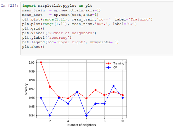
FIGURE 18-2: Validation curves.
You can obtain two pieces of information from the visualization:
- The peak cross-validation accuracy using nine neighbors is higher than the training score. The training score should always be better than any cross-validation score. The higher score points out that the example overfitted the cross-validation and luck played a role in getting such a good cross-validation score.
- The second peak of cross-validation accuracy, at five neighbors, is near the lowest results. Well-scoring areas usually surround optimum values, so this peak is a bit suspect.
Based on the visualization, you should accept the nine- neighbors solution (it is the highest and it is indeed surrounded by other acceptable solutions). As an alternative, given that nine neighbors is a solution on the limit of the search, you could instead launch a new grid search, extending the limit to a higher number of neighbors (above ten) in order to verify whether the accuracy stabilizes, decreases, or even improves.
It is part of the data science process to query, test, and query again. Even though Python and its packages offer you many automated processes in data learning and discovering, it is up to you to ask the right questions and to check whether the answers are the best ones by using statistical tests and visualizations.
Trying a randomized search
Grid searching, though exhaustive, is indeed a time-consuming activity. It’s prone to overfitting the cross-validation folds when you have few observations in your dataset and you extensively search for an optimization. Instead, an interesting alternative option is to try a randomized search. In this case, you define a grid search to test only some of the combinations, picked at random.
Even though it may sound like betting on blind luck, a grid search is actually quite useful because it’s inefficient — if you pick enough random combinations, you have a high statistical probability of finding an optimum hyperparameter combination, without risking overfitting at all. For instance, in the previous example, the code tested 40 different models using a systematic search. Using a randomized search, you can reduce the number of tests by 75 percent, to just 10 tests, and reach the same level of optimization!
Using a randomized search is straightforward. You import the class from the grid_search module and input the same parameters as the GridSearchCV, adding a n_iter parameter that indicates how many combinations to sample. As a rule of thumb, you choose from a quarter or a third of the total number of hyperparameter combinations:
from sklearn.model_selection import RandomizedSearchCV
random_search = RandomizedSearchCV(estimator=classifier,
param_distributions=grid, n_iter=10,
scoring=score_metric, n_jobs=1, refit=True, cv=10, )
random_search.fit(X, y)
Having completed the search using the same technique as before, you can explore the results by outputting the best scores and parameters:
print('Best parameters: %s' % random_search.best_params_)
print('CV Accuracy of best parameters: %.3f' %
random_search.best_score_)The resulting search ends with the following best parameters and score:Best parameters: {'n_neighbors': 9, 'weights': 'distance',
'p': 2}
Accuracy of best parameters: 0.973
From the reported results, it appears that a random search can actually obtain results similar to a much more CPU-expensive grid search.