
Chapter 2
Introducing Python’s Capabilities and Wonders
IN THIS CHAPTER
![]() Delving into why Python came about
Delving into why Python came about
![]() Getting a quick start with Python
Getting a quick start with Python
![]() Considering Python’s special features
Considering Python’s special features
![]() Defining and exploring the power of Python for the data scientist
Defining and exploring the power of Python for the data scientist
All computers run on just one language — machine code. However, unless you want to learn how to talk like a computer in 0s and 1s, machine code isn’t particularly useful. You’d never want to try to define data science problems using machine code. It would take an entire lifetime (if not longer) just to define one problem. Higher-level languages make it possible to write a lot of code that humans can understand quite quickly. The tools used with these languages make it possible to translate the human-readable code into machine code that the machine understands. Therefore, the choice of languages depends on the human need, not the machine need. With this in mind, this chapter introduces you to the capabilities that Python provides that make it a practical choice for the data scientist. After all, you want to know why this book uses Python and not another language, such as Java or C++. These other languages are perfectly good choices for some tasks, but they’re not as suited to meet data science needs.
The chapter begins with a short history of Python so that you know a little about why developers created Python in the first place. You also see some simple Python examples to get a taste for the language. As part of exploring Python in this chapter, you discover all sorts of interesting features that Python provides. Python gives you access to a host of libraries that are especially suited to meet the needs of the data scientist. In fact, you use a number of these libraries throughout the book as you work through the coding examples. Knowing about these libraries in advance will help you understand the programming examples and why the book shows how to perform tasks in a certain way.
 Even though this chapter does show examples of working with Python, you don’t really begin using Python in earnest until Chapter 6. This chapter provides you with an overview so that you can better understand what Python can do. Chapter 3 shows how to install the particular version of Python used for this book. Chapters 4 and 5 are about tools you can use, with Chapter 4 emphasizing Google’s Colab, an alternative environment for coding. In short, if you don’t quite understand an example in this chapter, don’t worry: You get plenty of additional information in later chapters.
Why Python?
Python is the vision of a single person, Guido van Rossum. You might be surprised to learn that Python has been around a long time — Guido started the language in December 1989 as a replacement for the ABC language. Not much information is available as to the precise goals for Python, but it does retain ABC’s ability to create applications using less code. However, it far exceeds the ability of ABC to create applications of all types, and in contrast to ABC, boasts four programming styles. In short, Guido took ABC as a starting point, found it limited, and created a new language without those limitations. It’s an example of creating a new language that really is better than its predecessor.
Python has gone through a number of iterations and currently has two development paths. The 2.x path is backward compatible with previous versions of Python, while the 3.x path isn’t. The compatibility issue is one that figures into how data science uses Python because a few of the libraries won’t work with 3.x. However, this issue is slowly being resolved, and you should use 3.x for all new development because the end of the line is coming for the 2.x versions (see https://pythonclock.org/ for details). As a result, this edition of the book uses 3.x code. In addition, some versions use different licensing because Guido was working at various companies during Python’s development. You can see a listing of the versions and their respective licenses at https://docs.python.org/3/license.html. The Python Software Foundation (PSF) owns all current versions of Python, so unless you use an older version, you really don’t need to worry about the licensing issue.
Grasping Python’s Core Philosophy
Guido actually started Python as a skunkworks project. The core concept was to create Python as quickly as possible, yet create a language that is flexible, runs on any platform, and provides significant potential for extension. Python provides all these features and many more. Of course, there are always bumps in the road, such as figuring out just how much of the underlying system to expose. You can read more about the Python design philosophy at http://python-history.blogspot.com/2009/01/pythons-design-philosophy.html. The history of Python at http://python-history.blogspot.com/2009/01/introduction-and-overview.html also provides some useful information.
Contributing to data science
Because this is a book about data science, you’re probably wondering how Python contributes toward better data science and what the word better actually means in this case. Knowing that a lot of organizations use Python doesn’t help you because it doesn’t really say much about how they use Python, and if you want to match your choice of language to your particular need, answering how they use Python becomes important.
One such example appears at https://www.datasciencegraduateprograms.com/python/. In this case, the article talks about Forecastwatch.com (https://forecastwatch.com/), which actually does watch the weather and try to make predictions better. Every day, Forecastwatch.com compares 36,000 forecasts with the actual weather that people experience and then uses the results to create better forecasts. Trying to aggregate and make sense of the weather data for 800 U.S. cities is daunting, so Forecastwatch.com needed a language that could do what it needed with the least amount of fuss. Here are the reasons Forecast.com chose Python:
- Library support: Python provides support for a large number of libraries, more than any one organization will ever need. According to
https://www.python.org/about/success/forecastwatch/, Forecastwatch.com found the regular expression, thread, object serialization, and gzip data compression libraries especially useful. - Parallel processing: Each of the forecasts is processed as a separate thread so that the system can work through them quickly. The thread data includes the web page URL that contains the required forecast, along with category information, such as city name.
- Data access: This huge amount of data can’t all exist in memory, so Forecast.com relies on a MySQL database accessed through the MySQLdb (
https://sourceforge.net/projects/mysql-python/) library, which is one of those few libraries that hasn’t moved on to Python 3.x yet. However, the associated website promises the required support soon. - Data display: Originally, PHP produced the Forecastwatch.com output. However, by using Quixote (
https://www.mems-exchange.org/software/quixote/), which is a display framework, Forecastwatch.com was able to move everything to Python.
Discovering present and future development goals
The original development (or design) goals for Python don’t quite match what has happened to the language since Guido initially thought about it. Guido originally intended Python as a second language for developers who needed to create one-off code but who couldn’t quite achieve their goals using a scripting language. The original target audience for Python was the C developer. You can read about these original goals in the interview at http://www.artima.com/intv/pyscale.html.
You can find a number of applications written in Python today, so the idea of using it solely for scripting didn’t come to fruition. In fact, you can find listings of Python applications at https://www.python.org/about/apps/ and https://www.python.org/about/success/. As of this writing, Python is the fourth-ranked language in the world (see https://www.tiobe.com/tiobe-index/). It continues to move up the scale because developers see it as one of the best ways to create modern applications, many of which rely on data science.
Naturally, with all these success stories to go on, people are enthusiastic about adding to Python. You can find lists of Python Enhancement Proposals (PEPs) at http://legacy.python.org/dev/peps/. These PEPs may or may not see the light of day, but they prove that Python is a living, growing language that will continue to provide features that developers truly need to create great applications of all types, not just those for data science.
Working with Python
This book doesn’t provide you with a full Python tutorial. (However, you can get a great start with Beginning Programming with Python For Dummies, 2nd Edition, by John Paul Mueller (Wiley). For now, it’s helpful to get a brief overview of what Python looks like and how you interact with it, as in the following sections.
 You don’t have to type the source code for this chapter manually. You’ll find using the downloadable source a lot easier (see the Introduction for details on downloading the source code). The source code for this chapter appears in the
 P4DS4D2_02_Using_Python.ipynb source code file.
Getting a taste of the language
Python is designed to provide clear language statements but to do so in an incredibly small space. A single line of Python code may perform tasks that another language usually takes several lines to perform. For example, if you want to display something on-screen, you simply tell Python to print it, like this:
print("Hello There!")
This is an example of a 3.x print() function. (The 2.x version of Python includes both a function form of print, which requires parentheses, and a statement form of print, which omits the parentheses.) The “Why Python?” section of this chapter mentions some differences between the 2.x path and the 3.x path. If you use the print() function without parentheses in 3.x, you get an error message:
File ">Jupyter-input-1-fe18535d9681>", line 1
print "Hello There!"
^
SyntaxError: Missing parentheses in call to 'print'. Did you
mean print("Hello There!")?
The point is that you can simply tell Python to output text, an object, or anything else using a simple statement. You don’t really need too much in the way of advanced programming skills. When you want to end your session using a command line environment such as IDLE, you simply type quit() and press Enter. This book relies on a much better environment, Jupyter Notebook, which really does make your code look as though it came from someone’s notebook.
Understanding the need for indentation
Python relies on indentation to create various language features, such as conditional statements. One of the most common errors that developers encounter is not providing the proper indentation for code. You see this principle in action later in the book, but for now, always be sure to pay attention to indentation as you work through the book examples. For example, here is an if statement (a conditional that says that if something meets the condition, perform the code that follows) with proper indentation.
if 1 > 2:
print("1 is less than 2")
 The
The print statement must appear indented below the conditional statement. Otherwise, the condition won’t work as expected, and you might see an error message, too.
Working at the command line or in the IDE
Anaconda is a product that makes using Python even easier. It comes with a number of utilities that help you work with Python in a variety of ways. The vast majority of this book relies on Jupyter Notebook, which is part of the Anaconda installation you create in Chapter 3. You saw this editor used in Chapter 1 and you see it again later in the book. In fact, this book doesn’t use any of the other Anaconda utilities much at all. However, they do exist, and sometimes they’re helpful in playing with Python. The following sections provide a brief overview of the other Anaconda utilities for creating Python code. You may want to experiment with them as you work through various coding techniques in the book.
Creating new sessions with Anaconda Command Prompt
Only one of the Anaconda utilities provides direct access to the command line, Anaconda Prompt. When you start this utility, you see a command prompt at which you can type commands. The main advantage of this utility is that you can start an Anaconda utility with any of the switches it provides to modify that utility’s standard environment. Of course, you start many of the utilities using the Python interpreter that you access using the python.exe command. (If you have both Python 3.6 and Python 2.7 installed on your system and open a regular command prompt or terminal window, you may see the Python 2.7 version start instead of the Python 3.6 version, so it’s always best to open an Anaconda Command Prompt to ensure that you get the right version of Python.) So you could simply type python and press Enter to start a copy of the Python interpreter should you wish to do so. Figure 2-1 shows how the plain Python interpreter looks.
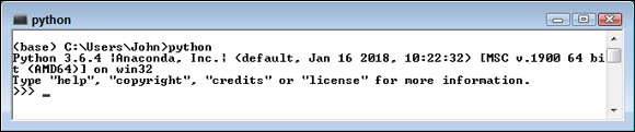
FIGURE 2-1: A view of the plain Python interpreter.
You quit the interpreter by typing quit() and pressing Enter. Once back at the command line, you can discover the list of python.exe command-line switches by typing python -? and pressing Enter. Figure 2-2 shows just some of the ways in which you can change the Python interpreter environment.

FIGURE 2-2: The Python interpreter includes all sorts of command-line switches.
If you want, you can create a modified form of any of the utilities provided by Anaconda by starting the interpreter with the correct script. The scripts appear in the scripts subdirectory. For example, type python Anaconda3/scripts/Jupyter-script.py and press Enter to start the Jupyter environment without using the graphical command for your platform. You can also add command-line arguments to further modify the script’s behavior. When working with this script, you can get information about Jupyter by using the following command-line arguments:
--version: Obtains the version of Jupyter Notebook in use.--config-dir: Displays the configuration directory for Jupyter Notebook (where the configuration information is stored).--data-dir: Displays the storage location of Jupyter application data, rather than projects. Your projects generally appear in your user folder.--runtime-dir: Shows the location of the Jupyter runtime files, which is normally a subdirectory of the data directory.--paths: Creates a list of paths that Jupyter is configured to use.
Consequently, if you want to obtain a list of Jupyter paths, you type python Anaconda3/scripts/Jupyter-script.py --paths and press Enter. The scripts subdirectory also contains a wealth of executable files. Often, these files are compiled versions of scripts and may execute more quickly as a result. If you want to start the Jupyter Notebook browser environment, you can either type python Anaconda3/scripts/Jupyter-notebook-script.py and press Enter to use the script version or execute Jupyter-notebook.exe. The result is the same in either case.
Entering the IPython environment
The Interactive Python (IPython) environment provides enhancements to the standard Python interpreter. To start this environment, you use the IPython command, rather than the standard Python command, at the Anaconda Prompt. The main purpose of the environment shown in Figure 2-3 is to help you use Python with less work. Note that the Python version is the same as when using the Python command, but that the IPython version is different and that you see a different prompt. To see these enhancements (as shown in the figure), type %quickref and press Enter.

FIGURE 2-3: The Jupyter environment is easier to use than the standard Python interpreter.
One of the more interesting additions to IPython is a fully functional clear screen (cls) command. You can’t clear the screen easily when working in the Python interpreter, which means that things tend to get a bit messy after a while. It’s also possible to perform tasks such as searching for variables using wildcard matches. Later in the book, you see how to use the magic functions to perform tasks such as capturing the amount of time it takes to perform a task for the purpose of optimization.
Entering Jupyter QTConsole environment
Trying to remember Python commands and functions is hard — and trying to remember the enhanced Jupyter additions is even harder. In fact, some people would say that the task is impossible (and perhaps they’re right). This is where the Jupyter QTConsole comes into play. It adds a graphical user interface (GUI) on top of Jupyter that makes using the enhancements that Jupyter provides a lot easier.
You may think that QTConsole is missing if you used previous versions of Anaconda, but it’s still present. Only the direct access method is gone. To start QTConsole, open an Anaconda Prompt, type Jupyter QTConsole, and press Enter. You see QTConsole start, as shown in Figure 2-4. Of course, you give up a little screen real estate to get this feature, and some hardcore programmers don’t like the idea of using a GUI, so you have to choose what sort of environment to work with when programming.

FIGURE 2-4: Use the QTConsole to make working with Jupyter easier.
Some of the enhanced commands appear in menus across the top of the window. All you need to do is choose the command you want to use. For example, to restart the kernel, you choose Kernel ⇒ Restart Current Kernel. You also have the same access to IPython commands. For example, type %magic and press Enter to see a list of magic commands.
Editing scripts using Spyder
Spyder is a fully functional Integrated Development Environment (IDE). You use it to load scripts, edit them, run them, and perform debugging tasks. Figure 2-5 shows the default windowed environment.

FIGURE 2-5: Spyder is a traditional style IDE for developers who need one.
The Spyder IDE is much like any other IDE that you might have used in the past. The left side contains an editor in which you type code. Any code you create is placed in a script file, and you must save the script before running it. The upper-right window contains various tabs for inspecting objects, exploring variables, and interacting with files. The lower-right window contains the Python console, a history log, and the Jupyter console. Across the top, you see menu options for performing all the tasks that you normally associate with working with an IDE.
Performing Rapid Prototyping and Experimentation
Python is all about creating applications quickly and then experimenting with them to see how things work. The act of creating an application design in code without necessarily filling in all the details is prototyping. Python uses less code than other languages to perform tasks, so prototyping goes faster. The fact that many of the actions you need to perform are already defined as part of libraries that you load into memory makes things go faster still.
Data science doesn’t rely on static solutions. You may have to try multiple solutions to find the particular solution that works best. This is where experimentation comes into play. After you create a prototype, you use it to experiment with various algorithms to determine which algorithm works best in a particular situation. The algorithm you use varies depending on the answers you see and the data you use, so there are too many variables to consider for any sort of canned solution.
 The prototyping and experimentation process occurs in several phases. As you go through the book, you discover that these phases have distinct uses and appear in a particular order. The following list shows the phases in the order in which you normally perform them.
- Building a data pipeline. To work with the data, you must create a pipeline to it. It’s possible to load some data into memory. However, after the dataset gets to a certain size, you need to start working with it on disk or by using other means to interact with it. The technique you use for gaining access to the data is important because it impacts how fast you get a result.
- Performing the required shaping. The shape of the data — the way in which it appears and its characteristics (such as data type), is important in performing analysis. To perform an apples-to-apples comparison, like data has to be shaped the same. However, just shaping the data the same isn’t enough. The shape has to be correct for the algorithms you employ to analyze it. Later chapters (starting with Chapter 7) help you understand the need to shape data in various ways.
- Analyzing the data. When analyzing data, you seldom employ a single algorithm and call it good enough. You can’t know which algorithm will produce the same results at the outset. To find the best result from your dataset, you experiment on it using several algorithms. This practice is emphasized in the later chapters of the book when you start performing serious data analysis.
- Presenting a result. A picture is worth a thousand words, or so they say. However, you need the picture to say the correct words or your message gets lost. Using the MATLAB-like plotting functionality provided by the
matplotliblibrary, you can create multiple presentations of the same data, each of which describes the data graphically in different ways. To ensure that your meaning really isn’t lost, you must experiment with various presentation methods and determine which one works best.
Considering Speed of Execution
Computers are known for their prowess in crunching numbers. Even so, analysis takes considerable processing power. The datasets are so large that you can bog down even an incredibly powerful system. In general, the following factors control the speed of execution for your data science application:
- Dataset size: Data science relies on huge datasets in many cases. Yes, you can make a robot see objects using a modest dataset size, but when it comes to making business decisions, larger is better in most situations. The application type determines the size of your dataset in part, but dataset size also relies on the size of the source data. Underestimating the effect of dataset size is deadly in data science applications, especially those that need to operate in real time (such as self-driving cars).
- Loading technique: The method you use to load data for analysis is critical, and you should always use the fastest means at your disposal, even if it means upgrading your hardware to do so. Working with data in memory is always faster than working with data stored on disk. Accessing local data is always faster than accessing it across a network. Performing data science tasks that rely on Internet access through web services is probably the slowest method of all. Chapter 6 helps you understand loading techniques in more detail. You also see the effects of loading technique later in the book.
- Coding style: Some people will likely try to tell you that Python’s programming paradigms make writing a slow application nearly impossible. They’re wrong. Anyone can create a slow application using any language by employing coding techniques that don’t make the best use of programming language functionality. To create fast data science applications, you must use best-of-method coding techniques. The techniques demonstrated in this book are a great starting point.
- Machine capability: Running data science applications on a memory-constrained system with a slower processor is impossible. The system you use needs to have the best hardware you can afford. Given that data science applications are both processor and disk bound, you can’t really cut corners in any area and expect great results.
- Analysis algorithm: The algorithm you use determines the kind of result you obtain and controls execution speed. Many of the chapters in the latter parts of this book demonstrate multiple methods to achieve a goal using different algorithms. However, you must still experiment to find the best algorithm for your particular dataset.
A number of the chapters in this book emphasize performance, most notably speed and reliability, because both factors are critical to data science applications. Even though database applications tend to emphasize the need for speed and reliability to some extent, the combination of huge dataset access (disk-bound issues) and data analysis (processor-bound issues) in data science applications makes the need to make good choices even more critical.
Visualizing Power
Python makes it possible to explore the data science environment without resorting to using a debugger or debugging code, as would be needed in many other languages. The print statement (or function, depending on the version of Python you use) and dir() function let you examine any object interactively. In short, you can load something up and play with it for a while to see just how the developer put it together. Playing with the data, visualizing what it means to you personally, can often help you gain new insights and create new ideas. Judging by many online conversations, playing with the data is the part of data science that its practitioners find the most fun.
You can play with data using any of the tools found in Anaconda, but one of the best tools for the job is IPython (see the “Entering the IPython environment” section, earlier in of this chapter, for details) because you don’t really have to worry too much about the environment, and nothing you create is permanent. After all, you’re playing with the data. Therefore, you can load a dataset to see just what it has to offer, as shown in Figure 2-6. Don’t worry if this code looks foreign and hard to understand right now. Beginning with Chapter 4, you start to play with code more, and the various sections give you more details. You can also obtain the book Beginning Programming with Python For Dummies, 2nd Edition, by John Paul Mueller (Wiley) if you want a more detailed tutorial. Just follow along with the concept of playing with data for now.
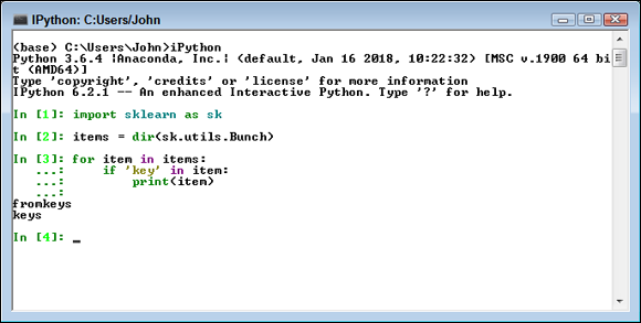
FIGURE 2-6: Load a dataset and play with it a little.
Scikit-learn datasets appear within bunches (a bunch is a kind of data structure). When you import a dataset, that dataset will have certain functions that you can use with it that are determined by the code used to define the datastructure — a bunch. This code shows which functions deal with keys — the data identifiers for the values (one or more columns of information) in the dataset. Each row in the dataset has a unique key, even if the values in that row repeat another row in the dataset. You can use these functions to perform useful work with the dataset as part of building your application.
Before you can work with a dataset, you must provide access to it in the local environment. Figure 2-7 shows the import process and demonstrates how you can use the keys() function to display a list of keys that you can use to access data within the dataset.

FIGURE 2-7: Use a function to learn more information.
When you have a list of keys you can use, you can access individual data items. For example, Figure 2-8 shows a list of all the feature names contained in the Boston dataset. Python really does make it possible to know quite a lot about a dataset before you have to work with it in depth.

FIGURE 2-8: Access specific data using a key.
Using the Python Ecosystem for Data Science
You have already seen the need to load libraries in order to perform data science tasks in Python. The following sections provide an overview of the libraries you use for the data science examples in this book. Various book examples show the libraries at work.
Accessing scientific tools using SciPy
The SciPy stack (http://www.scipy.org/) contains a host of other libraries that you can also download separately. These libraries provide support for mathematics, science, and engineering. When you obtain SciPy, you get a set of libraries designed to work together to create applications of various sorts. These libraries are
- NumPy
- SciPy
- matplotlib
- Jupyter
- Sympy
- pandas
The SciPy library itself focuses on numerical routines, such as routines for numerical integration and optimization. SciPy is a general-purpose library that provides functionality for multiple problem domains. It also provides support for domain-specific libraries, such as Scikit-learn, Scikit-image, and statsmodels.
Performing fundamental scientific computing using NumPy
The NumPy library (http://www.numpy.org/) provides the means for performing n-dimensional array manipulation, which is critical for data science work. The Boston dataset used in the examples in Chapters 1 and 2 is an example of an n-dimensional array, and you couldn’t easily access it without NumPy functions that include support for linear algebra, Fourier transform, and random-number generation (see the listing of functions at http://docs.scipy.org/doc/numpy/reference/routines.html).
Performing data analysis using pandas
The pandas library (http://pandas.pydata.org/) provides support for data structures and data analysis tools. The library is optimized to perform data science tasks especially fast and efficiently. The basic principle behind pandas is to provide data analysis and modeling support for Python that is similar to other languages, such as R.
Implementing machine learning using Scikit-learn
The Scikit-learn library (http://scikit-learn.org/stable/) is one of a number of Scikit libraries that build on the capabilities provided by NumPy and SciPy to allow Python developers to perform domain-specific tasks. In this case, the library focuses on data mining and data analysis. It provides access to the following sorts of functionality:
- Classification
- Regression
- Clustering
- Dimensionality reduction
- Model selection
- Preprocessing
A number of these functions appear as chapter headings in the book. As a result, you can assume that Scikit-learn is the most important library for the book (even though it relies on other libraries to perform its work).
Going for deep learning with Keras and TensorFlow
Keras (https://keras.io/) is an application programming interface (API) that is used to train deep learning models. An API often specifies a model for doing something, but it doesn’t provide an implementation. Consequently, you need an implementation of Keras to perform useful work, which is where TensorFlow (https://www.tensorflow.org/) comes into play. You can also use Microsoft’s Cognitive Toolkit, CNTK (https://www.microsoft.com/en-us/cognitive-toolkit/), or Theano (https://github.com/Theano), to implement Keras, but this book focuses on TensorFlow.
When working with an API, you’re looking for ways to simplify things. Keras makes things easy in the following ways:
- Consistent interface: The Keras interface is optimized for common use cases with an emphasis on actionable feedback for fixing user errors.
- Lego approach: Using a black-box approach makes it easy to create models by connecting configurable building blocks together with only a few restrictions on how you can connect them.
- Extendable: You can easily add custom building blocks to express new ideas for research that include new layers, loss functions, and models.
- Parallel processing: To run applications fast today, you need good parallel processing support. Keras runs on both CPUs and GPUs.
- Direct Python support: You don’t have to do anything special to make the TensorFlow implementation of Keras work with Python, which can be a major stumbling block when working with other sorts of APIs.
Plotting the data using matplotlib
The matplotlib library (http://matplotlib.org/) gives you a MATLAB-like interface for creating data presentations of the analysis you perform. The library is currently limited to 2-D output, but it still provides you with the means to express graphically the data patterns you see in the data you analyze. Without this library, you couldn’t create output that people outside the data science community could easily understand.
Creating graphs with NetworkX
To properly study the relationships between complex data in a networked system (such as that used by your GPS setup to discover routes through city streets), you need a library to create, manipulate, and study the structure of network data in various ways. In addition, the library must provide the means to output the resulting analysis in a form that humans understand, such as graphical data. NetworkX (https://networkx.github.io/) enables you to perform this sort of analysis. The advantage of NetworkX is that nodes can be anything (including images) and edges can hold arbitrary data. These features allow you to perform a much broader range of analysis with NetworkX than using custom code would (and such code would be time consuming to create).
Parsing HTML documents using Beautiful Soup
The Beautiful Soup library (http://www.crummy.com/software/BeautifulSoup/) download is actually found at https://pypi.python.org/pypi/beautifulsoup4/4.3.2. This library provides the means for parsing HTML or XML data in a manner that Python understands. It allows you to work with tree-based data.
Besides providing a means for working with tree-based data, Beautiful Soup takes a lot of the work out of working with HTML documents. For example, it automatically converts the encoding (the manner in which characters are stored in a document) of HTML documents from UTF-8 to Unicode. A Python developer would normally need to worry about things like encoding, but with Beautiful Soup, you can focus on your code instead.