Chapter 6: Colorspaces, Transformations, and Thresholding

In the previous chapter, we learned how to perform basic mathematical and logical operations on images. In this chapter, we will continue to explore some more intriguing concepts in the area of computer vision and its applications in the real world. Just like in the earlier chapters of this book, we will have a lot of hands-on exercises with Python 3 and create many real-world apps. We will cover a very wide variety of advanced topics in the area of computer vision. The major topics we will learn about are related to colorspaces, transformations, and thresholding images. After completing this chapter, you will be able to write programs for a few basic real-world applications, such as tracking an object that's a specific color. You will also be able to apply geometric and perspective transformations to images and live USB webcam feeds.

In this chapter, we will explore the following topics:

• Colorspaces and converting them
• Performing transformation operations on images
• Perspective transformation of images
• Thresholding images

Technical requirements

The code files of this chapter can be found on GitHub at https://github.com/PacktPublishing/raspberry-pi-computer-vision-programming/tree/master/Chapter06/programs.

Check out the following video to see the Code in Action at https://bit.ly/384oYqM.

Colorspaces and converting them

Let's understand the concept of a colorspace. A colorspace is a mathematical model that is used to represent a set of colors. With colorspaces, we can represent colors with numbers. If you've ever have worked with web programming, then you must have come across various codes for colors since colors are represented in HTML with Hexadecimal numbers. This is a good example of representing colors with a colorspace and allows us to perform numerical and logical computations with them. Representing colors with colorspaces also allows us to reproduce the colors with ease in analog and digital forms.

We will frequently use BGR, RGB, HSV, and grayscale colorspaces throughout this book. In BGR and RGB, B stands for blue, G stands for green, and R stands for red. OpenCV reads and stores a color image in the BGR colorspace. The HSV colorspace represents a set of colors with a component for hue, a component for saturation, and a component for value. It is a very commonly used colorspace in the areas of computer graphics and computer vision. OpenCV has a function, cv2.cvtColor(img, conv_flag), that changes the colorspace of the image that's passed to it as an argument. The source and target colorspaces are denoted by the argument that's passed to the conv_flag parameter. This function converts the numerical value of a color from the source colorspace into the target colorspace with the use of mathematical formulae used for colorspace conversion.

Note:

You can read more about colorspaces and conversion at the following URL: http://colorizer.org.

As you may recall, earlier, in Chapter 4, Getting Started with Computer Vision, we discussed that OpenCV loads images in BGR format and that Matplotlib uses the RGB format for images. So, when we display images read by OpenCV in BGR format with matplotlib in RGB format, the red and blue channels are interchanged in the visualization and the image looks funny. We should convert an image from BGR into RGB before displaying the image with matplotlib. There are two ways to do this.

Let's look at the first way. We can split the image into B, G, and R channels and merge them into an RGB image with the split() and merge() functions, as follows:

import cv2

import matplotlib.pyplot as plt

img = cv2.imread('/home/pi/book/dataset/4.2.07.tiff', 1)

b,g,r = cv2.split (img)

img = cv2.merge((r, g, b))

plt.imshow (img)

plt.title ('COLOR IMAGE')

plt.axis('off')

plt.show()

However, the split and merge operations are computationally expensive. A better approach is to use the cv2.cvtColor() function to change the colorspace of an image from BGR to RGB, as demonstrated in the following code:

import cv2

import matplotlib.pyplot as plt

img = cv2.imread('/home/pi/book/dataset/4.2.07.tiff', 1)

img = cv2.cvtColor (img, cv2.COLOR_BGR2RGB)

plt.imshow (img)

plt.title ('COLOR IMAGE')

plt.axis('off')

plt.show()

In the preceding code, we used the cv2.COLOR_BGR2RGB flag for color conversion. OpenCV has plenty of such flags for color conversion. We can run the following program to see the entire list:

import cv2

j=0

for filename in dir(cv2):

if filename.startswith('COLOR_'):

print(filename)

j = j + 1

print('There are ' + str(j) +

' Colorspace Conversion flags in OpenCV '

+ cv2.__version__ + '.')

The last few lines of the output are shown in the following code block (I am not including the entire output due to space limitations):

.

.

.

.

.

COLOR_YUV420p2RGBA

COLOR_YUV420sp2BGR

COLOR_YUV420sp2BGRA

COLOR_YUV420sp2GRAY

COLOR_YUV420sp2RGB

COLOR_YUV420sp2RGBA

COLOR_mRGBA2RGBA

There are 274 colorspace conversion flags in OpenCV 4.0.1.

HSV colorspace

The term HSV stands for hue, saturation, and value. In this colorspace or color model, a color is represented by the hue (also known as the tint), the shade (which is the saturation scale or the amount of gray with white and black on extreme ends), and the brightness (the value or the luminescence). The intensities of the colors red, yellow, green, cyan, blue, and magenta are represented by the hue. The term saturation means the amount of gray component present in the color. The brightness or the intensity of the color is represented by the value component.

The following code converts a color from BGR into HSV and prints it:

import cv2

import numpy as np

c = cv2.cvtColor(np.array([[[255, 0, 0]]],

dtype=np.uint8),

cv2.COLOR_BGR2HSV)

print(c)

The preceding code snippet will print the HSV value of blue represented in BGR. The following is the output:

[[[120 255 255]]]

We will heavily use the HSV colorspace throughout this book. Before proceeding further, let's create a small app with a trackbar that adjusts the saturation of the color when the tracker moves:

import cv2

def emptyFunction():

pass

img = cv2.imread('/home/pi/book/dataset/4.2.07.tiff', 1)

windowName = "Saturation Demo"

cv2.namedWindow(windowName)

cv2.createTrackbar('Saturation Level',

windowName, 0,

24, emptyFunction)

while(True):

hsv = cv2.cvtColor( img, cv2.COLOR_BGR2HSV)

h, s, v = cv2.split(hsv)

saturation = cv2.getTrackbarPos('Saturation Level', windowName)

s = s + saturation

v = v + saturation

img1 = cv2.cvtColor(cv2.merge((h, s, v)), cv2.COLOR_HSV2BGR)

cv2.imshow(windowName, img1)

if cv2.waitKey(1) == 27:

break

cv2.destroyAllWindows()

In the preceding code, we first converted the image from BGR into HSV and split it into H, S, and V components. Then, we added a number to saturation (s), as well as a value (v), based on the position of the tracker in the trackbar. Then, we merged all the channels to create an HSV image and then converted it back into BGR to be displayed with the cv2.imshow() function. The following is a screenshot of the output window:

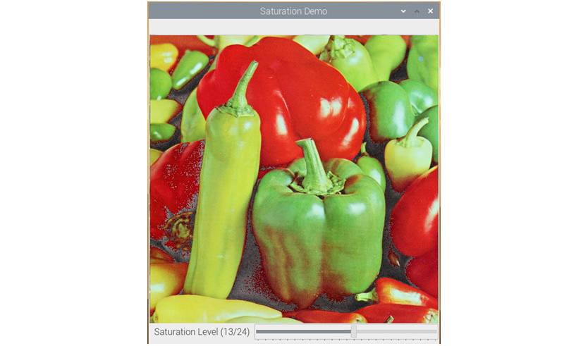
Figure 6.1 – App for adjusting the saturation of an image

Tracking in real time based on color

Now, let's learn how to demonstrate the concept of converting colorspaces to implement a real-life mini project. The HSV colorspace makes it easy for us to work with a range of a color. To track an object that can have colors in a specific range, we need to convert the image's colorspace into HSV and check if any part of the image falls within the specific range of the color we are interested in. OpenCV has a function, cv2.inRange(), that offers the functionality to define a color range.

This function accepts an image and the upper bound and the lower bound of the range of the color as arguments. Then, it checks if any pixel of the given image falls within the range of color (the upper bound and the lower bound). If the pixel value in the image lies in the given range of color, the corresponding pixel in the output image is set to the value 0; otherwise, it is set to the value 255. This creates a binary image that can be used as a mask for computing the logical operations that we will use for tracking the application.

The following example demonstrates this concept. We are using the logical bitwise_and() function to extract the range of the color we are interested in:

import numpy as np

import cv2

cap = cv2.VideoCapture(0)

while ( True ):

ret, frame = cap.read()

hsv = cv2.cvtColor(frame, cv2.COLOR_BGR2HSV)

image_mask = cv2.inRange(hsv, np.array([40, 50, 50]),

np.array([80, 255, 255]))

output = cv2.bitwise_and(frame, frame, mask=image_mask)

cv2.imshow('Original', frame)

cv2.imshow('Output', output)

if cv2.waitKey(1) == 27:

break

cv2.destroyAllWindows()

cap.release()

In this program, we are tracking the green-colored objects. The output should look like what's shown in the following screenshot. Here, I used the lid (cover) of a container, which is a greenish color:

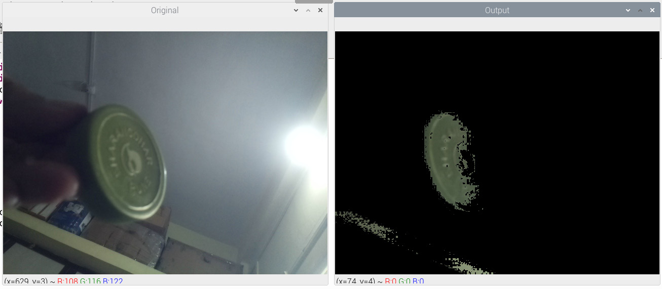
Figure 6.2 – Tracking an object by color in real time

The parts of the wall also have a greenish tint. Due to this, they are also visible in the output.

I have not included the intermediate mask image we computed in the preceding output. We can view it in a separate output window by adding the following line of code to the code we wrote earlier:

cv2.imshow('Image Mask', image_mask)

This mask is purely black and white, also known as a binary image. If we make modifications to the preceding code, we can track objects that have distinct colors. We must create another mask for the range of colors we are interested in. Then, we can combine both masks, as follows:

blue = cv2.inRange(hsv, np.array([100, 50, 50]), np.array([140, 255, 255]))

green = cv2.inRange(hsv, np.array([40, 50, 50]), np.array([80, 255, 255]))

image_mask = cv2.add(blue, green)

output = cv2.bitwise_and(frame, frame, mask=image_mask)

Run this code and check the output for yourself. We can add a trackbar to this code to select a range of blue or green colors. The following are the steps to do this:

1. First, import all the required libraries:

   import numpy as np

   import cv2

2. Then, we define an empty function:

   def emptyFunction():

   pass

3. Let's initialize all the required objects and variables:

   cap = cv2.VideoCapture(0)

   windowName = 'Object Tracker'

   trackbarName = 'Color Chooser'

   cv2.namedWindow(windowName)

   cv2.createTrackbar(trackbarName,

   windowName, 0, 1,

   emptyFunction)

   color = 0

4. Here, we have the main loop:

   while (True):

   ret, frame = cap.read()

   hsv = cv2.cvtColor(frame, cv2.COLOR_BGR2HSV)

   color = cv2.getTrackbarPos(trackbarName, windowName)

   if color == 0:

   image_mask = cv2.inRange(hsv, np.array([40, 50, 50]),

   np.array([80, 255, 255]))

   else:

   image_mask = cv2.inRange(hsv, np.array([100, 50, 50]),

   np.array([140, 255, 255]))

   output = cv2.bitwise_and(frame, frame, mask=image_mask)

   cv2.imshow(windowName, output)

   if cv2.waitKey(1) == 27:

   break

5. Finally, we destroy all the windows and release the camera:

   cv2.destroyAllWindows()

   cap.release()

Run the preceding code and see the output for yourself. By now we are aware of the GPIO interface and the push buttons. As an exercise, try to implement the same functionality with the push buttons so that there will be separate push buttons for tracking blue and green colors.

Performing transformation operations on images

In this section, we will learn how to perform various mathematical transformation operations on images with OpenCV and Python 3.

Scaling

Scaling means resizing an image. It is a geometric operation. OpenCV offers a function, cv2.resize(), for performing this operation. It accepts an image, a method for the interpolation of pixels, and the scaling factor as arguments and returns a scaled image. The following methods are used for the interpolation of the pixels in the output:

• cv2.INTER_LANCZOS4: This deals with the Lanczos interpolation method over a neighborhood of 8x8 pixels.
• cv2.INTER_CUBIC: This deals with the bicubic interpolation method over a neighborhood of 4x4 pixels and is preferred for performing the zooming operation on an image.
• cv2.INTER_AREA: This means resampling using pixel area relation. This is preferred for performing the shrinking operation on an image.
• cv2.INTER_NEAREST: This means the method of nearest-neighbor interpolation.
• cv2.INTER_LINEAR: This means the method of bilinear interpolation. This is the default argument for the parameter.

The following example demonstrates performing upscaling and downscaling on an image:

import cv2

img = cv2.imread('/home/pi/book/dataset/house.tiff', 1)

upscale = cv2.resize(img, None, fx=1.5, fy=1.5,

interpolation=cv2.INTER_CUBIC)

downscale = cv2.resize(img, None, fx=0.5, fy=0.5,

interpolation=cv2.INTER_AREA)

cv2.imshow('upscale', upscale)

cv2.imshow('downscale', downscale)

cv2.waitKey(0)

cv2.destroyAllWindows()

In the preceding code, we first upscale in both axes and then downscale in both axes by factors of 1.5 and 0.5, respectively. Run the preceding code to see the output. Also, as an exercise, try to pass different numbers as scaling factors.

The translation, rotation, and affine transformation of images

The cv2.warpAffine() function is used to compute operations such as translation, rotation, and affine transformations on input images. It accepts an input image, the matrix of the transformation, and the size of the output image as arguments, and then it returns the transformed image.

Note:

You can find out more about the mathematical aspects of affine transformations at http://mathworld.wolfram.com/AffineTransformation.html.

The following examples demonstrate different types of mathematical transformations that can be applied to images with the cv2.warpAffine() function. The translation operation means changing (more precisely, shifting) the location of the image in the XY reference plane. The shifting factor in the x and y axes can be represented with a two-dimensional transformation matrix, T, as follows:

The following code shifts the location of the image in the XY plane by a factor of (-50, 50):

import numpy as np

import cv2

import matplotlib.pyplot as plt

img = cv2.imread('/home/pi/book/dataset/house.tiff', 1)

input=cv2.cvtColor(img, cv2.COLOR_BGR2RGB)

rows, cols, channel = img.shape

T = np.float32([[1, 0, -50], [0, 1, 50]])

output = cv2.warpAffine(input, T, (cols, rows))

plt.imshow(output)

plt.title('Shifted Image')

plt.show()

The output of the preceding code is as follows:

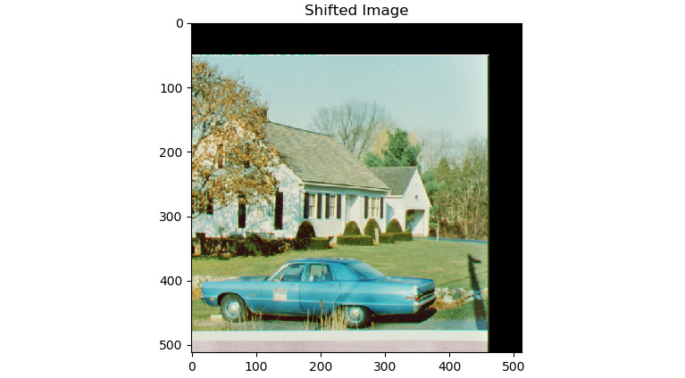
Figure 6.3 – Output of the translation operation

As shown in the preceding output, a part of the image in the output is cropped (or truncated), since the size of the output window is the same as the input window, and the original image has shifted beyond the first quadrant of the XY plane. Similarly, we can use the cv2.warpAffine() function to apply the operation of rotation with scaling to an input image. For this demonstration, we must define a matrix of the rotation using the cv2.getRotationMatrix2D() function.

This accepts the angle of anti-clockwise rotation in degrees, the center of the rotation, and the scaling factor as arguments. Then, it creates a matrix of the rotation operation that can be passed as an argument to the call of the cv2.warpAffine() function. The following example applies the rotation operation to an input image with 45 degrees as the angle of the rotation and the center of the image as the center of the rotation operation, and it also scales the output image down to half (50%) the size of the original input image:

import cv2

import matplotlib.pyplot as plt

img = cv2.imread('/home/pi/book/dataset/house.tiff', 1)

input = cv2.cvtColor(img, cv2.COLOR_BGR2RGB)

rows, cols, channel = img.shape

R = cv2.getRotationMatrix2D((cols/2, rows/2), 45, 0.5)

output = cv2.warpAffine(input, R, (cols, rows))

plt.imshow(output)

plt.title('Rotated and Downscaled Image')

plt.show()

The output will be as follows:

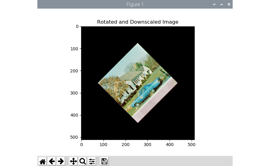
Figure 6.4 – Output of the rotation operation

We can also create a very nice animation by modifying the preceding program. The trick here is that, in the while loop, we must change the angle of rotation at a regular interval and show those frames successively to create the rotation effect on a still image. The following code example demonstrates this:

import cv2

from time import sleep

image = cv2.imread('/home/pi/book/dataset/house.tiff',1)

rows, cols, channels = image.shape

angle = 0

while(1):

if angle == 360:

angle = 0

M = cv2.getRotationMatrix2D((cols/2, rows/2), angle, 1)

rotated = cv2.warpAffine(image, M, (cols, rows))

cv2.imshow('Rotating Image', rotated)

angle = angle +1

sleep(0.2)

if cv2.waitKey(1) == 27 :

break

cv2.destroyAllWindows()

Run the preceding code and check the output for yourself. Now, let's try to implement this trick on a live webcam. Use the following code to do so:

import cv2

from time import sleep

cap = cv2.VideoCapture(0)

ret, frame = cap.read()

rows, cols, channels = frame.shape

angle = 0

while(1):

ret, frame = cap.read()

if angle == 360:

angle = 0

M = cv2.getRotationMatrix2D((cols/2, rows/2), angle, 1)

rotated = cv2.warpAffine(frame, M, (cols, rows))

cv2.imshow('Rotating Image', rotated)

angle = angle +1

sleep(0.2)

if cv2.waitKey(1) == 27 :

break

cv2.destroyAllWindows()

Run the preceding code and see it in action.

Now, let's learn about the concept of the affine mathematical transformation and demonstrate the same with OpenCV and Python 3. An affine transformation is a geometric mathematical transformation that ensures that the parallel lines in the original input image remain parallel in the output image. The usual inputs to the affine transformation operation are a set of three points that are not in the same line in the input image and the corresponding set of three points that are not in the same line in the output image. These sets of points are passed to the cv2.getAffineTransform() function to compute the transformation matrix, and that computed transformation matrix, in turn, is passed to the call of the cv2.warpAffine() function as an argument. The following example demonstrates this concept very well:

import cv2

import numpy as np

from matplotlib import pyplot as plt

image = cv2.imread('/home/pi/book/dataset/4.2.06.tiff', 1)

input = cv2.cvtColor(image, cv2.COLOR_BGR2RGB )

rows, cols, channels = input.shape

points1 = np.float32([[100, 100], [300, 100], [100, 300]])

points2 = np.float32([[200, 150], [400, 150], [100, 300]])

A = cv2.getAffineTransform(points1, points2)

output = cv2.warpAffine(input, A, (cols, rows))

plt.subplot(121)

plt.imshow(input)

plt.title('Input')

plt.subplot(122)

plt.imshow(output)

plt.title('Affine Output')

plt.show()

The following is the output:

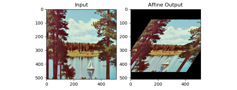
Figure 6.5 – Affine transformation

As we can see, the preceding code creates a shear-like effect on the input image.

Perspective transformation of images

In the mathematical operation of perspective transformation, a set of four points in the input image is mapped to a set of four points in the output image. The criteria for selecting the set of four points in the input and the output image is that any three points (in the input and the output image) must not be in the same line. Like affine mathematical transformation, in perspective transformation, the straight lines in the input images remain straight. However, there is no guarantee that the parallel lines in the input image remain parallel in the output image.

One of the most prominent real-life examples of this mathematical operation is the zoom and the angled zoom functions in image editing and viewing software tools. The amount of zoom and angle of zooming depend on the matrix of the transformation that is computed by the two sets of points that we discussed earlier. OpenCV provides the cv2.getPerspectiveTransform() function, which accepts two sets of four points from the input image and the output image and computes the matrix of the transformation. The cv2.warpPerspective() function accepts the computed matrix as an argument and applies it to the input image to compute the perspective transform of the input image. The following code demonstrates this aptly:

import cv2

import numpy as np

from matplotlib import pyplot as plt

image = cv2.imread('/home/pi/book/dataset/ruler.512.tiff', 1)

input = cv2.cvtColor(image, cv2.COLOR_BGR2RGB )

rows, cols, channels = input.shape

points1 = np.float32([[0, 0], [400, 0], [0, 400], [400, 400]])

points2 = np.float32([[0,0], [300, 0], [0, 300], [300, 300]])

P = cv2.getPerspectiveTransform(points1, points2)

output = cv2.warpPerspective(input, P, (300, 300))

plt.subplot(121)

plt.imshow(input)

plt.title('Input Image')

plt.subplot(122)

plt.imshow(output)

plt.title('Perspective Transform')

plt.show()

The output will appear as follows:

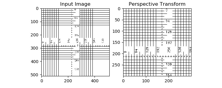
Figure 6.6 – Zoom operation with perspective transform

As an exercise for this section (and to improve your understanding of the operation of perspective transformation), pass various combinations of sets of points in the input and the output images to the program to see how the output changes when the input is changed. From the example we just discussed, you may get the impression that the parallelism between the lines in the input and the output image is preserved, but that is because of our choice of sets for the points in the input image and the output image. If we choose different sets of points, then the output will obviously be different.

These are all the transformation operations we can perform on images with OpenCV. Next, we will see how to threshold images with OpenCV.

Thresholding images

Thresholding is the simplest way to divide images into various parts, which are known as segments. Thresholding is the simplest form of segmentation operation. If we apply the thresholding operation to a grayscale image, it is usually (but not all the time) transformed into a binary image. A binary image is a strictly black and white image and it can either have a 0 (black) or 255 (white) value for a pixel. Many segmentation algorithms, advanced image processing operations, and computer vision applications use thresholding as the first step for processing images.

Thresholding is perhaps the simplest image processing operation. First, we must define a value for the threshold. If a pixel has a value greater than the threshold, then we assign 255 (white) to that pixel; otherwise, we assign 0 (black) to the pixel. This is the simplest way we can implement the thresholding operation on an image. There are other thresholding techniques too, and we will learn about and demonstrate them in this section.

The OpenCV cv2.threshold() function applies thresholding to images. It accepts the image, the value of the threshold, the maximum value, and the technique of thresholding as arguments and returns the thresholded image as the output. This function assigns the value of the maximum value to a pixel if its value is greater than the value of the threshold. As we mentioned earlier, there are variations of this method. Let's take a look at all the thresholding techniques in detail.

Let's assume that (x, y) is the input pixel. Here, we can threshold an image in the following ways:

• cv2.THRESH_BINARY: If intensity(x, y) > thresh, then set intensity(x, y) = maxVal; otherwise, set intensity(x, y) = 0.
• cv2.THRESH_BINARY_INV: If intensity(x, y) > thresh, then set intensity(x, y) = 0; otherwise, set intensity(x, y) = maxVal.
• cv2.THRESH_TRUNC: If intensity(x, y) > thresh, then set intensity(x, y) = threshold; else leave intensity(x, y) as it is.
• cv2.THRESH_TOZERO: If intensity(x, y)> thresh; then leave intensity(x, y) as it is; otherwise, set intensity(x, y) = 0.
• cv2.THRESH_TOZERO_INV: If intensity(x, y) > thresh, then set intensity(x, y) = 0; otherwise, leave intensity(x, y) as it is.

Grayscale images with gradients are excellent input for thresholding algorithms as we can visually see the thresholding in action. In the following example, we are using a grayscale gradient image as an input to demonstrate the thresholding operation. We have set the value of the threshold to 127, so the image is segmented into two or more parts, depending on the value of the intensity of pixels and thresholding technique that we are using:

import cv2

import matplotlib.pyplot as plt

import numpy as np

img = cv2.imread('/home/pi/book/dataset/gray21.512.tiff', 1)

th = 127

max_val = 255

ret, o1 = cv2.threshold(img, th, max_val,

cv2.THRESH_BINARY)

print(o1)

ret, o2 = cv2.threshold(img, th, max_val,

cv2.THRESH_BINARY_INV)

ret, o3 = cv2.threshold(img, th, max_val,

cv2.THRESH_TOZERO)

ret, o4 = cv2.threshold(img, th, max_val,

cv2.THRESH_TOZERO_INV)

ret, o5 = cv2.threshold(img, th, max_val,

cv2.THRESH_TRUNC)

titles = ['Input Image', 'BINARY', 'BINARY_INV',

'TOZERO', 'TOZERO_INV', 'TRUNC']

output = [img, o1, o2, o3, o4, o5]

for i in range(6):

plt.subplot(2, 3, i+1)

plt.imshow(output[i], cmap='gray')

plt.title(titles[i])

plt.axis('off')

plt.show()

The following is the output:

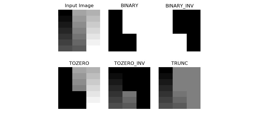
Figure 6.7 – Output of the thresholding operation

You might want to create an application with a trackbar. We can also interface two push buttons in the pull-up configuration and write some code to adjust the threshold on a live video with the help of those two push buttons:

import RPi.GPIO as GPIO

import cv2

thresh = 127

cap = cv2.VideoCapture(0)

GPIO.setmode(GPIO.BOARD)

GPIO.setwarnings(False)

button1 = 7

button2 = 11

GPIO.setup(button1, GPIO.IN, GPIO.PUD_UP)

GPIO.setup(button2, GPIO.IN, GPIO.PUD_UP)

while True:

ret, frame = cap.read()

button1_state = GPIO.input(button1)

if button1_state == GPIO.LOW and thresh < 256:

thresh = thresh + 1

button2_state = GPIO.input(button2)

if button2_state == GPIO.LOW and thresh > -1:

thresh = thresh - 1

ret1, output = cv2.threshold(frame, thresh, 255,

cv2.THRESH_BINARY)

print(thresh)

cv2.imshow('Thresholding App', output)

if cv2.waitKey(1) == 27:

break

cv2.destroyAllWindows()

Prepare a circuit by connecting two push buttons to pins 7 and 11. Connect a webcam to a USB or Pi Camera Module to the CSI port. Then, run the preceding code. The following will be the output:

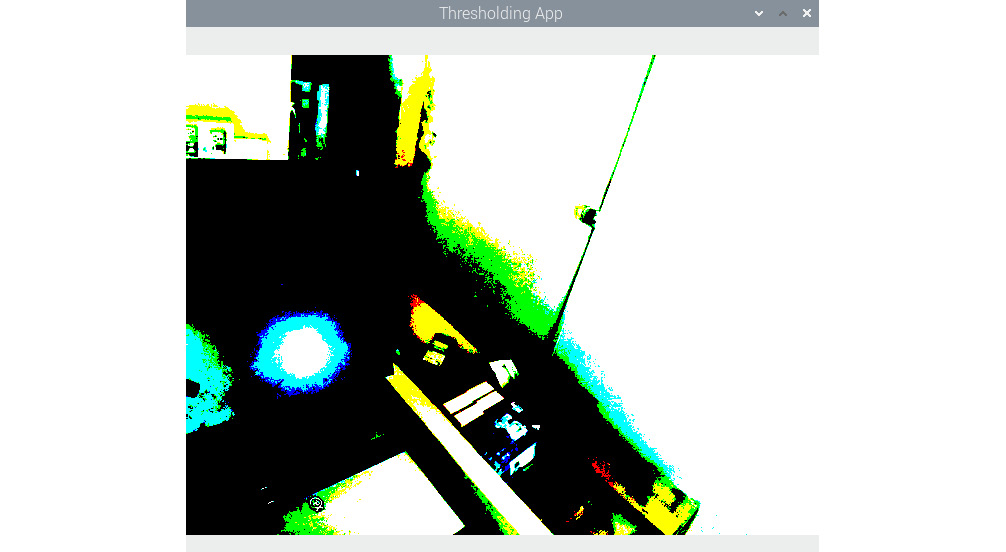
Figure 6.8 – Thresholding a live USB webcam feed

The output looks like this because we are applying thresholding to the live feed and the color image. OpenCV applies thresholding to all the channels. As an exercise, convert the input frame into grayscale and then apply different types of thresholds to it.

Otsu's binarization method

In our previous examples of thresholding, we chose the value of the thresholding argument. However, the value of the threshold for the input image is a technique that's automatically determined by Otsu's binarization method. However, this method does not work for all images. The prerequisite is that the input image must have two peaks in the histogram. Such images are known as bimodal histogram images. We will learn more about this concept and demonstrate how to use histograms and histograms of images later in this book. A bimodal histogram usually means that the image has a background and a foreground. Otsu's binarization works best with such images.

This method is not recommended for images other than those that have bimodal histograms as it will produce improper results. This method is always combined with other thresholding methods. While calling the cv2.threshold() function, we have to pass 0 as an argument to the threshold parameter, as shown in the following code snippet:

ret, output = cv2.threshold(image, 0, 255, cv2.THRESH_BINARY + cv2.THRESH_OTSU )

Run the preceding code and see the output.

Adaptive thresholding

In the earlier examples (including Otsu's binarization), the threshold is the same for all the pixels in the entire image. That is why those techniques are known as global thresholding techniques. However, they do not produce good results for all types of images. For images where lighting is not uniform, global thresholding methods are not the best. We can use algorithms that compute the threshold values locally, depending on the value of the nearby pixel. Such techniques are known as local or adaptive thresholding techniques.

The cv2.adaptiveThreshold() method accepts a source image, maximum value, adaptive thresholding method, thresholding algorithm, block size, and a constant as inputs and produces a thresholded image as output. The following shows how to use the mean and Gaussian methods for deciding on the neighborhood in order to determine a threshold value:

import cv2

import matplotlib.pyplot as plt

img = cv2.imread('/home/pi/book/dataset/4.1.05.tiff', 0)

block_size = 123

constant = 6

th1 = cv2.adaptiveThreshold(img, 255,

cv2.ADAPTIVE_THRESH_MEAN_C,

cv2.THRESH_BINARY,

block_size, constant)

th2 = cv2.adaptiveThreshold (img, 255,

cv2.ADAPTIVE_THRESH_GAUSSIAN_C,

cv2.THRESH_BINARY,

block_size, constant)

output = [img, th1, th2]

titles = ['Original', 'Mean Adaptive', 'Gaussian Adaptive']

for i in range(3):

plt.subplot(1, 3, i+1)

plt.imshow(output[i], cmap='gray')

plt.title(titles[i])

plt.xticks([])

plt.yticks([])

plt.show()

The following is the output of the preceding code:

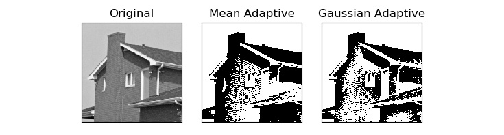
Figure 6.9 – Mean and Gaussian adaptive thresholding methods

As we can see in the preceding output image, the outputs produced by the mean and Gaussian adaptive threshold are different. We must choose the proper thresholding algorithm based on the input image to get the desired results. Often, a trial and error method is the best for choosing the thresholding algorithms and the value of the threshold.

Summary

This was an interesting chapter. We started by looking at colorspaces and their application for object tracking by color. Then, we learned about transformations and thresholding. We also learned how to create a small app with push buttons for live thresholding. All the concepts we demonstrated, especially thresholding techniques, will be very useful for the advanced image processing applications we will learn about later in this book.

In the next chapter, we will learn about a few signal processing concepts and image noise. We will learn about techniques for filtering images and removing noise in images. We will also combine those concepts with the RPi's GPIO and create a few nice live image processing apps.