Chapter 9: Image Restoration, Segmentation, and Depth Maps

In the previous chapter, we demonstrated how to use high-pass filters and their applications in algorithms to detect edges.

In this chapter, we will learn about a few more advanced processing techniques regarding images. First, we will get started with the restoration of damaged or degraded images. Then, we will explore the fundamentals of various types of segmentation techniques. We have already seen that thresholding is a basic form of segmentation. We will explore this concept in more detail in this chapter. Finally, we will compute the disparity map and estimate the depths of objects in an image.

In this chapter, we will cover the following topics:

• Restoring damaged images using inpainting
• Segmenting images
• Disparity maps and depth estimation

By the end of this chapter, we will be able to restore damaged images, apply various segmentation algorithms to images, and estimate the depth of objects using disparity maps.

Technical requirements

The code files of this chapter can be found on GitHub at https://github.com/PacktPublishing/raspberry-pi-computer-vision-programming/tree/master/Chapter09/programs.

Check out the following video to see the Code in Action at https://bit.ly/2NsIzXY.

Restoring damaged images using inpainting

The restoration of an image is the computational process of reconstructing damaged parts from existing parts of an image. If we capture an image on film with a photographic camera and develop it on paper, the photographic paper tends to degrade with the passage of time, leading to degradation of the photograph. Faulty sensors and imperfections such as dust and dirt on the camera lenses can introduce errors in the captured image. The process of transmission and reception can also introduce errors in the digital image. Image inpainting techniques can restore degraded and damaged images. Many algorithms are available to repair images. The OpenCV library implements two of the repairing methods using the cv2.inpaint() function.

This function accepts a degraded or damaged source image, a mask for image inpainting, the size of the inpainting neighborhood, and the inpainting method as arguments. The mask of inpainting is the damaged area represented by a grayscale image where white pixels refer to the area to be repaired or inpainted. The following code demonstrates both of the methods that we discussed above. The output produced by both methods is almost the same. We can create the damaged mask using free image editing software such as GIMP. Take a look at the following code:

import cv2

import matplotlib.pyplot as plt

image = cv2.imread('/home/pi/book/dataset/Damaged.tiff')

mask = cv2.imread('/home/pi/book/dataset/Mask.tiff', 0)

input = cv2.cvtColor(image, cv2.COLOR_BGR2RGB)

output_TELEA = cv2.inpaint(input, mask, 5, cv2.INPAINT_TELEA)

output_NS = cv2.inpaint(input, mask, 5, cv2.INPAINT_NS)

plt.subplot(221)

plt.imshow(input)

plt.title('Damaged Image')

plt.axis('off')

plt.subplot(222)

plt.imshow(mask, cmap='gray'),

plt.title('Mask')

plt.axis('off')

plt.subplot(223),

plt.imshow(output_TELEA)

plt.title('Telea Method')

plt.axis('off')

plt.subplot(224)

plt.imshow(output_NS)

plt.title('Navier Stokes Method')

plt.axis('off')

plt.show()

In the preceding code, we have used two techniques. The cv2.INPAINT_TELEA flag is based on a technique described in the paper named An Image Inpainting Technique Based on the Fast Marching Method, which was written and published in 2004 by Alexandru Telea.

The cv2.INPAINT_NS flag is based on a technique described in the paper Navier-Stokes, Fluid Dynamics, and Image and Video Inpainting, which was written and published in 2001 by Bertalmio Marcelo, Andrea L. Bertozzi, and Guillermo Sapiro.

The following is the output:

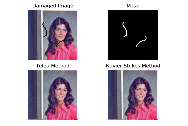
Figure 9.1 – The restoration of degraded images

In the preceding output, the first image is the damaged image. The second image is the binary mask corresponding to the damage. The images in the second row are the restored images using the Telea method and the Navier-Stokes method.

Note

You can find out more about image inpainting at https://www.math.ucla.edu/~imagers/htmls/inp.html.

Segmenting images

The segmentation of images is the process of dividing images into many sections or parts, also known as segments. This process is carried out using particular criteria. The simplest way in which we can divide images into segments is through thresholding. We have already learned about and demonstrated the techniques of thresholding in Chapter 6, Colorspaces, Transformations, and Thresholding. We will demonstrate two more methods of segmentation in this chapter. Those methods are the Mean Shift algorithm and k-means clustering.

Mean shift algorithm segmentation

Bogdan Georgescu and Chris M. Christoudias developed the mean shift algorithm and implemented it in C++. The Python implementation of the same algorithm is known as PyMeanShift. PyMeanShift uses ndarrays and NumPy for storing and processing images. That is why it is compatible with NumPy-based image processing libraries such as OpenCV, Mahotas, and scikit-image.

Note

You can find out more about this on the project GitHub page at https://github.com/fjean/pymeanshift.

There is no binary package for the installation of PyMeanShift on Linux, Unix, and other operating systems based on them. We must build it and install it from the source. Download the latest version of the source code from this URL: https://github.com/fjean/pymeanshift. The download will be a ZIP file. Copy it to the home directory of the pi user, /pi/home, and extract it. Navigate to the directory where we extracted it and run the following commands in order on LXTerminal:

cd ~

cd pymeanshift-master/

sudo python3 setup.py build

sudo python3 setup.py install

Once the installation is complete, run the following command on Command Prompt to check whether it was successful:

python3 -c "import pymeanshift as pms"

The pymeanshift library offers the pms.segment() function, which segments the images represented by NumPy ndarrays. It accepts the source input image to be segmented, the spatial radius, the radius of the range, and the minimum density as arguments. Then, it returns a segmented image, a labeled color image, and a set of regions. The following is the code example to demonstrate the functionality:

import cv2

import pymeanshift as pms

from matplotlib import pyplot as plt

img = cv2.imread('/home/pi/book/dataset/house.tiff', 1)

input = cv2.cvtColor(img, cv2.COLOR_BGR2RGB )

(segmented_image, labels_image, number_regions) = pms.segment(

input, spatial_radius=2, range_radius=2, min_density=300)

plt.subplot(131)

plt.imshow(input)

plt.title('Input')

plt.axis('off')

plt.subplot(132)

plt.imshow(segmented_image)

plt.title('Segmented Output')

plt.axis('off')

plt.subplot(133)

plt.imshow(labels_image)

plt.title('Labeled Output')

plt.axis('off')

plt.show()

The output of the preceding code is as follows:

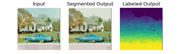
Figure 9.2 – Segmentation with PyMeanShift

As an exercise, pass different values of arguments to the function parameters and compare the output. We can apply this to a live feed video from a webcam as follows:

import cv2

import pymeanshift as pms

cap = cv2.VideoCapture(0)

while True:

ret, frame = cap.read()

(segmented_image, labels_image, number_regions) = pms.segment(

frame, spatial_radius=2, range_radius=2, min_density=50)

cv2.imshow('Segmented', segmented_image)

if cv2.waitKey(1) == 27:

break

cv2.destroyAllWindows()

cap.release()

Usually, the segmentation is computationally a very expensive operation and, therefore, the frames per second (FPS) for a live video is very low. The output of this will be similar to the previous one (Figure 2).

K-means clustering and image quantization

The k-means clustering algorithm is a classification algorithm. Suppose that the input to the algorithm is a set of size n, and then the output divides that set into k number of partitions. That is why it is known as the k-means algorithm. Essentially, based on particular criteria, we are dividing or classifying the data into k number of classes or partitions. When this is applied to the data with two or more dimensions (that is, multidimensional data), it is called clustering. OpenCV has the cv2.kmeans() function that implements the k-means clustering algorithm for single-dimensional and multidimensional data. It accepts the arguments for the following parameters:

• Data: This is the input data to the k-means clustering algorithm. This data must be in the floating-point numerical format.
• K: The total number of partitions in the output of the algorithm. It must be known in advance (if the input is the color image, this will mean the number of colors in the output segmented image).
• Criteria: The termination criteria for the algorithm.
• Attempts: The number of times the algorithm is run with the different initial labels.
• Flags: This signifies the position of the initial centers for the clusters, which are passed in any one of the following values as arguments:

  cv2.KMEANS_RANDOM_CENTERS

  cv2.KMEANS_PP_CENTERS

  cv2.KMEANS_USE_INITIAL_LABELS

Let's try to demonstrate this program for one-dimensional data first. We will create our own random data for this. Let's create and visualize the data:

import numpy as np

import cv2

from matplotlib import pyplot as plt

x = np.random.randint(25, 100, 25)

y = np.random.randint(175, 255, 25)

z = np.hstack((x, y))

z = z.reshape((50, 1))

z = np.float32(z)

plt.hist(z, 256, [0, 256])

plt.show()

The sample random data will look like the following output:

Figure 9.3 – One-dimensional data

We can clearly see the data divided into two groups. Now, let's make Raspberry Pi classify it and highlight the groups and their centers. Remove or comment out the last two lines of the preceding code and add the following lines:

criteria = (cv2.TERM_CRITERIA_EPS +

cv2.TERM_CRITERIA_MAX_ITER, 10, 1.0)

flags = cv2.KMEANS_RANDOM_CENTERS

compactness, labels, centers = cv2.kmeans(z, 2,

None,

criteria,

10, flags)

A = z[labels==0]

B = z[labels==1]

plt.hist(A, 256, [0, 256], color = 'g')

plt.hist(B, 256, [0, 256], color = 'b')

plt.hist(centers, 32, [0, 256], color = 'r')

plt.show()

Let's run the preceding program. Note that we are rerunning the calls to the np.random.randint() functions so the dataset will be slightly different. Nevertheless, it will have two different groups, which are highlighted as follows:

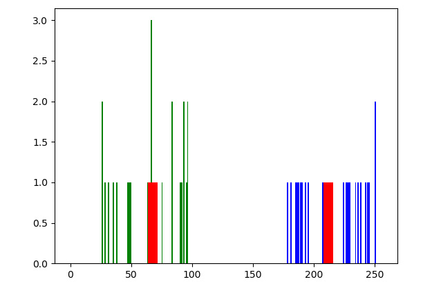
Figure 9.4 – K-means applied to one-dimensional data

We can implement this method in two-dimensional data as follows:

import numpy as np

import cv2

from matplotlib import pyplot as plt

X = np.random.randint(25, 50, (25, 2))

Y = np.random.randint(60, 85, (25, 2))

Z = np.vstack((X, Y))

Z = np.float32(Z)

criteria = (cv2.TERM_CRITERIA_EPS +

cv2.TERM_CRITERIA_MAX_ITER, 10, 1.0)

ret,label,center=cv2.kmeans(Z, 2, None, criteria,

10, cv2.KMEANS_RANDOM_CENTERS)

A = Z[label.ravel()==0]

B = Z[label.ravel()==1]

plt.scatter(A[:,0], A[:,1])

plt.scatter(B[:,0], B[:,1], c = 'g')

plt.scatter(center[:,0], center[:,1],

s = 80, c = 'r', marker = 's')

plt.xlabel('X - Axis')

plt.ylabel('Y - Axis')

plt.show()

The output is as follows:

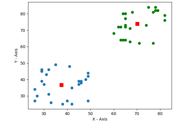
Figure 9.5 – K-means on two-dimensional data

In the preceding output, we can clearly see our data clustered into two groups. Let's write the code that applies the k-means clustering algorithm to a color image with the values for the sizes of k as 2, 4, and 12:

import cv2

import matplotlib.pyplot as plt

import numpy as np

img = cv2.imread('/home/pi/book/dataset/4.2.03.tiff', 1)

img = cv2.cvtColor(img, cv2.COLOR_BGR2RGB)

Z = img.reshape((-1, 3))

Z = np.float32(Z)

criteria = (cv2.TERM_CRITERIA_EPS +

cv2.TERM_CRITERIA_MAX_ITER,

10, 1.0)

In the preceding code, we are reading the image in color mode and reshaping it. We are also converting it into 32-bit float format. Then, we are setting the criteria for clustering in the last line.

Let's compute the quantized image with the value of k as 2, as follows:

k = 2

ret, label1, center1 = cv2.kmeans(Z, k, None, criteria, 10,

cv2.KMEANS_RANDOM_CENTERS)

center1=np.uint8(center1)

res1 = center1[label1.flatten()]

output1 = res1.reshape((img.shape))

In the previous code, we are computing the clusters with the cv2.kmeans() function and then flattening and reshaping them after converting the data into an 8-bit integer format.

Let's now compute the quantized image as follows with the value of k as 4:

k = 4

ret, label1, center1 = cv2.kmeans(Z, k, None, criteria, 10,

cv2.KMEANS_RANDOM_CENTERS)

center1=np.uint8(center1)

res1 = center1[label1.flatten()]

output2 = res1.reshape((img.shape))

Let's now compute the quantized image as follows with the value of k as 12:

k = 12

ret, label1, center1 = cv2.kmeans(Z, k, None, criteria, 10,

cv2.KMEANS_RANDOM_CENTERS)

center1=np.uint8(center1)

res1 = center1[label1.flatten()]

output3 = res1.reshape((img.shape))

Finally, let's display all the images in a grid using matplotlib:

output = [img, output1, output2, output3]

titles = ['Original Image', 'K=2', 'K=4', 'K=12']

for i in range(4):

plt.subplot(2, 2, i+1)

plt.imshow(output[i])

plt.title(titles[i])

plt.xticks([])

plt.yticks([])

plt.show()

In the preceding code, initially, we are assigning random centers to all the clusters using the cv2.KMEANS_RANDOM_CENTERS flag. The following output of the program we wrote has the original image and the segmented images using quantization, with 2, 4, and 12 colors. The following is the output:

Figure 9.6 – K-means clustering and image quantization

As an exercise, run the preceding program with different values of the arguments to the functions and compare the outputs. It will be interesting to implement this on the live video from a webcam. Do not expect a high frame rate as it is computationally very expensive.

Comparison of k-means and the mean shift algorithm

The k-means algorithm has a time complexity of O(n). The mean shift segmentation algorithm has a time complexity of O(n2). This difference of complexity is because the k-means algorithm provides the number of clusters through the argument at runtime. The mean shift segmentation algorithm must compute the number of clusters by itself at the time of execution. In applications where we do not know the number of clusters, we must use the mean shift algorithm. However, when we do know the number of clusters already, it is recommended that you use the k-means algorithm as it runs considerably faster when the number of clusters is known in advance.

Disparity maps and depth estimation

Disparity refers to the difference in the location of an object in the images captured by the left and right eyes or cameras. This difference or disparity is caused by parallax. Our brain uses this information regarding disparity to estimate the depth of objects (that is, their distance from us). We can compute the disparity between two images by applying this principle to every pixel in the pair of images captured by a webcam. This disparity information can be used to compute the estimated depth, thus mimicking the functionality of the brains of primates.

In terms of biology, this is known as Stereoscopic Vision, which enables us to see in three dimensions. OpenCV offers a cv2.StereoBM,compute() function that accepts the left image and the right image as an argument and returns a disparity map of the image pair. The StereoBM_create() function initializes the stereo state. It can have a number of disparities and block sizes as arguments. By default, they are 0 and 21, respectively. In the following example, we are calling this with default arguments. This stereo state is used to calculate the map of the disparities with the cv2.StereoBM.compute() functions. We need two images as inputs. One of these images corresponds to the input of the right camera, and the other corresponds to the input of the left camera. The following code demonstrates this concept using both functions:

import cv2

import matplotlib.pyplot as plt

Right= cv2.imread('/home/pi/book/dataset/imRsmall.jpg', 0)

Left = cv2.imread('/home/pi/book/dataset/imLsmall.jpg', 0)

stereo_BM_state=cv2.StereoBM_create()

output_map=stereo_BM_state.compute(Left, Right)

titles=['Left', 'Right', 'Depth Map']

output=[Left, Right, output_map]

for i in range(3):

plt.subplot(1, 3, i+1)

plt.imshow(output[i], cmap='gray')

plt.title(titles[i])

plt.axis('off')

plt.show()

The output of the preceding code will be as follows:

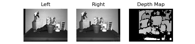
Figure 9.7 – Estimation of depth from the disparity map

In the preceding output, the brighter area in the output disparity map signifies more disparity. It means that objects in the source input image that correspond to the brighter areas in the output map of disparities are closer to the camera. Similarly, the darker colors in the output map of disparities signify that the object corresponding to those areas in the source input image is further away from the camera.

Summary

In this chapter, we learned about the concept of image inpainting and the restoration of damaged and degraded images. Then, we demonstrated many methods for the segmentation of images, including the mean shift algorithm and k-means clustering. Finally, we looked at how to estimate the depths of objects in images using disparity maps. All of these techniques are useful in many real-life applications. For example, whenever we want to send images over the network, we can use image quantization so that it consumes less bandwidth.

In the next chapter, we will learn about a few more advanced concepts such as histograms, the histograms of grayscale and color images, the detection of contours in images, and mathematical morphological operations.