Chapter 11: Real-Life Applications of Computer Vision

In the previous chapter, we studied various advanced concepts in computer vision such as morphological operations and contours.

This chapter is the culmination of all the computer vision concepts we've learned and demonstrated in the earlier chapters. In this chapter, we will use the computer vision operation we learned about earlier in detail to implement a few real-life projects. We will also learn about a few new concepts such as background subtraction and the computation of optical flow and then demonstrate them for small applications. This chapter contains a lot of hands-on programming examples, as well as detailed explanations of the code and new functionality.

In this chapter, we will learn and demonstrate the code for the following topics:

• Implementing the Max RGB filter
• Implementing background subtraction
• Computing the optical flow
• Detecting and tracking motion
• Detecting barcodes in images
• Implementing the chroma key effect

After completing this chapter, you will be able to implement the concepts you've learned about to create real-life applications such as security systems and motion detection systems using the Raspberry Pi (RPi) and some camera sensors.

Technical requirements

The code files of this chapter can be found on GitHub at https://github.com/PacktPublishing/raspberry-pi-computer-vision-programming/tree/master/Chapter11/programs.

Check out the following video to see the Code in Action at https://bit.ly/2Z43syb.

Implementing the Max RGB filter

We know that filters allow and block signals or data, depending on some criteria. Let's manually write the code for implementing a special filter based on the value of the intensity of the colors of pixels. This is known as the Max RGB filter. In a Max RGB filter, we compare the intensities of all the color channels of a color image for every pixel.

Then, we keep the intensity of the channel(s) with the maximum intensity and reduce the intensities of all the other channels to zero. This happens for every pixel in an image. Suppose, for a pixel, the intensities are (30, 200, 120). Then, after applying the Max RGB filter, it will be (0, 200, 0). Let's take a look at a program that will implement this with the NumPy and OpenCV functions:

import cv2

import numpy as np

def maxRGB(img):

    b = img[:, :, 0]

    g = img[:, :, 1]

    r = img[:, :, 2]

    M = np.maximum(np.maximum(b, g), r)

    b[b < M] = 0

    g[g < M] = 0

    r[r < M] = 0

    return(cv2.merge((b, g, r)))

cap = cv2.VideoCapture(0)

while True:

    ret, frame = cap.read()

    cv2.imshow('Max RGB Filter', maxRGB(frame))

    if cv2.waitKey(1) == 27:

        break

cv2.destroyAllWindows()

cap.release()

Run the preceding program and view the output. It is interesting to see the filtered live feed. The output looks as follows:

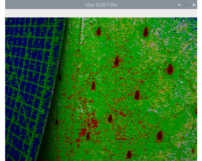
Figure 11.1 – Output of a Max RGB filter

In the next section, we will learn and demonstrate the concept of background subtraction.

Implementing background subtraction

Static cameras are used in many applications, such as security and monitoring. We can separate the background and moving objects by applying a process known as background subtraction. It usually returns a binary image with the background (the static part of the scene) in black pixels and the moving (changing or dynamic) parts in white pixels. OpenCV can implement this through two algorithms. The first is createBackgroundSubtractorKNN(). This creates a K-Nearest Neighbour (KNN) background subtractor object. Then, we can call the apply() function with the object to obtain the foreground mask. We can directly display the foreground mask in real time.

The following is a demonstration of how to use it:

import cv2

import numpy as np

cap = cv2.VideoCapture(0)

fgbg = cv2.createBackgroundSubtractorKNN()

while(True):

    ret, frame = cap.read()

    fgmask = fgbg.apply(frame)

    cv2.imshow('frame', fgmask)

    if cv2.waitKey(30) == 27:

        break

cap.release()

cv2.destroyAllWindows()

The output is a binary video stream, as shown in the following screenshot. I am waving my hand, which is highlighted by white pixels:

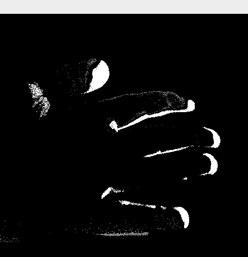
Figure 10.2 – Background subtraction with KNN

Note that if you keep your hand still for some time, OpenCV will consider it as a part of the background and will slowly dissolve it in the output.

Another similar function is cv2.createBackgroundSubtractorMOG2(). This also generates the foreground mask using the apply() function. The following is a sample program using it:

import cv2

import numpy as np

cap = cv2.VideoCapture(0)

fgbg = cv2.createBackgroundSubtractorMOG2()

while(True):

    ret, frame = cap.read()

    fgmask = fgbg.apply(frame)

    cv2.imshow('frame', fgmask)

    if cv2.waitKey(30) == 27:

        break

cap.release()

cv2.destroyAllWindows()

Run the preceding program and view the output. In both programs, we are creating the fgbg object and using the apply() function to compute the foreground mask, that is, fgmask. Then, we are just displaying the foreground mask in real time with the imshow() function. The expected output of this code can be seen in the preceding screenshot. Run the program and view the output for yourself.

Computing the optical flow

Optical flow (also known as optic flow) is the pattern that appears in the motion of objects in a video (live or recorded). Pay attention to the word appearance in the previous sentence. This means that if the observer (in our case, the camera) is in motion, then the objects in the scene are also considered to be moving, even if they are static. This is known as relative motion. In brief, the optical flow highlights the relative motion in the video. OpenCV has implementations for many of the functions that can compute the optical flow. The cv2.calcOpticalFlowFarneback() function computes the optical flow with the dense method. This means that it computes the flow for all the points. This function implements the Gunner Farneback algorithm.

NOTE:

You can read more about the Gunner Farneback argument at the following URL:

http://www.diva-portal.org/smash/get/diva2:273847/FULLTEXT01.pdfTwo-Frame

Let's see how we can compute the optical flow with OpenCV and Python 3 with the following code:

import cv2

import numpy as np

cap = cv2.VideoCapture(0)

ret, frame1 = cap.read()

prvs = cv2.cvtColor(frame1,

                    cv2.COLOR_BGR2GRAY)

hsv = np.zeros_like(frame1)

hsv[..., 1] = 255

while(cap):

    ret, frame2 = cap.read()

    next = cv2.cvtColor(frame2,

                        cv2.COLOR_BGR2GRAY)

    flow = cv2.calcOpticalFlowFarneback(prvs,

                                       next,

                                       None, 0.5,

                                       3, 15,

                                       3, 5,

                                       1.2, 0)

    mag, ang = cv2.cartToPolar(flow[..., 0],

                               flow[..., 1])

    hsv[..., 0] = ang * 180/np.pi/2

    hsv[..., 2] = cv2.normalize(mag, None, 0,

                                255, cv2.NORM_MINMAX)

    rgb = cv2.cvtColor(hsv, cv2.COLOR_HSV2BGR)

    cv2.imshow('Optical Flow', rgb)

    if cv2.waitKey(1) == 27:

        break

    prvs = next

cap.release()

cv2.destroyAllWindows()

In the preceding program, cv2.calcOpticalFlowFarneback() returns the coordinates of flow in the XY (Cartesian) system. We then convert it into polar with the cv2.cartToPolar() function. Then, the hue shows the angle of the motion and the value shows the intensity of the motion in the final HSV frame, which is converted into BGR and shown as output. The output will look like what's shown in the preceding screenshot. The only difference will be that the optical flow will be denoted by various colors.

The concept of the optical flow has applications in the following areas:

• Object detection and tracking
• Movement detection and tracking
• Navigation of robots

Detecting and tracking motion

Let's build a system for detecting and tracking motion in real time with the RPi, OpenCV, and Python. We will use a very simple technique to detect motion. Basically, we will compute the difference between the successive frames of a video feed (a video file or a live feed from a USB webcam). Then, we will plot contours around the area of pixels where we wish to detect the difference between successive frames:

1. We will begin by importing OpenCV and NumPy. Also, initialize an object corresponding to the USB webcam:

   import cv2

   import numpy as np

   cap = cv2.VideoCapture(0)

2. We will apply the dilation operation to the frames in the video. We need a kernel for that. We will define it before the video loop. Let's define it as follows:

   k = np.ones((3, 3), np.uint8)

3. The following code captures and stores the successive frames in separate variables:

   t0 = cap.read()[1]

   t1 = cap.read()[1]

4. Now, let's write the block for the while loop. In this block, we compute the absolute difference between the frames we captured earlier. We are going to use the cv2.absdiff() function for this. Then, we will convert the computed absolute difference into grayscale to process it further:

   while(True):

   d=cv2.absdiff(t1, t0)

   grey = cv2.cvtColor(d, cv2.COLOR_BGR2GRAY)

   The following is the output of the preceding code. It shows the grayscale of the absolute difference between the successively captured frames:

   

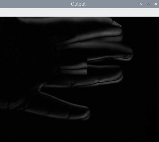
   Figure 11.3 – Absolute difference between successive frames

5. The output that we computed in the previous step has some noise. Due to this, we must blur it first with the Gaussian blurring technique to remove the noise:

   blur = cv2.GaussianBlur(grey, (3, 3), 0)

6. We apply the technique of binary thresholding to transform the blurred output from the previous step into a binary image for further processing with the following code:

   ret, th = cv2.threshold(blur, 15, 255, cv2.THRESH_BINARY)

7. Now, let's apply the dilation morphological operation to this binary image. This makes it easy to detect the boundaries in the thresholded image:

   dilated = cv2.dilate(th, k, iterations=2)

   The following is the output of the dilation operation:

   

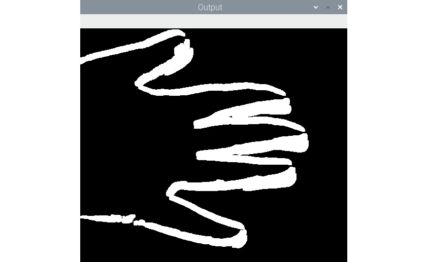
   Figure 11.4 – Dilated output

8. Let's go ahead and find the contours in the dilated image:

   contours, hierarchy = cv2.findContour(dilated,

   cv2.RETR_TREE,

   cv2.CHAIN_APPROX_SIMPLE)

   t2=t0

   cv2.drawContours(t2, contours, -1, (0, 255, 0), 2)

   cv2.imshow('Output', t2)

9. Now, let's copy the latest frame to the variable holding the older frame and then capture the next frame with the webcam:

   t0=t1

   t1=cap.read()[1]

   We end the while loop when the Esc key on the keyboard is pressed:

   if cv2.waitKey(5) == 27 :

   break

   Once the while loop ends, we perform the usual cleaning-up tasks such as releasing the camera capture object and destroying the display window:

   cap.release()

   cv2.destroyAllWindows()

   The following is the output of executing the program:

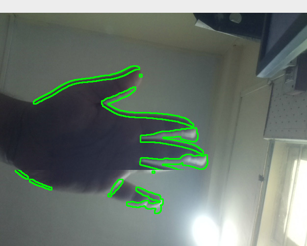
Figure 11.5 – Detected and highlighted movement

Keep in mind that this code is computationally expensive. Do not expect a very high framerate on the older and non-overclocked models of the RPi. As an exercise, draw contours of different colors. We can also compute the centroid with the help of the cv2.moments() function and represent those with small circles. This will make the output more interesting.

Detecting barcodes in images

A barcode is a way that information is represented visually and is easy to understand for purpose-made machines. There are many barcode formats. The usual format has parallel vertical lines of different thicknesses and different amounts of space in between them.

In this section, we will demonstrate how to detect a simple parallel-lines formatted barcode from a still image. We will use the following image of a soda can:

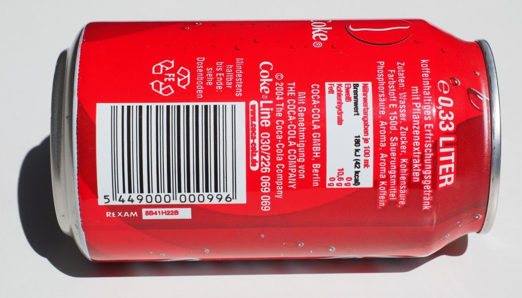
Figure 11.6 – The original source image

1. Let's read the source image of a soda can using the following code:

   import numpy as np

   import cv2

   image=cv2.imread('/home/pi/book/dataset/barcode.jpeg', 1)

   input = cv2.cvtColor(image, cv2.COLOR_BGR2GRAY)

2. The horizontal image of a barcode has a low and a high vertical gradient. So, the candidate image must have the region that fits this criterion. We will use the cv2.Sobel() function to compute the horizontal and vertical derivatives and then compute the difference to find out the region that fits the criteria. Let's see how to do that:

   hor_der = cv2.Sobel(input, ddepth=-1, dx=1, dy=0, ksize = 5)

   ver_der = cv2.Sobel(input, ddepth=-1, dx=0, dy=1, ksize=5)

   diff = cv2.subtract(hor_der, ver_der)

3. OpenCV provides the cv2.convertScaleAbs() function. It converts any numeric array into an array of 8-bit unsigned integers. Let's use it, as follows:

   diff = cv2.convertScaleAbs(diff)

   The output is as follows:

   

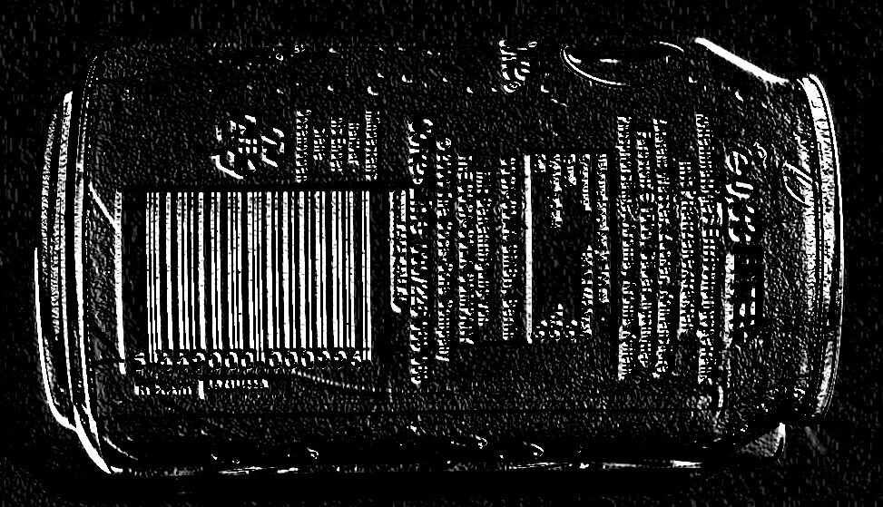
   Figure 11.7 – Difference between horizontal and vertical Sobel derivatives

4. The preceding output shows regions with very horizontal and very low vertical gradients. Let's apply a Gaussian blur to remove noise from the preceding output. Use the following code to do so:

   blur = cv2.GaussianBlur(diff, (3, 3), 0)

   The following is the output of the preceding code:

   

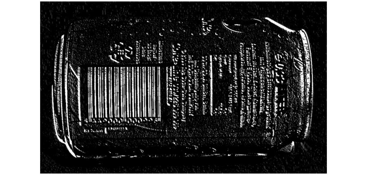
   Figure 11.8 – After applying a Gaussian blur

5. Now, let's convert this image into a binary image by applying thresholding to it. The following is the code to do so:

   ret, th = cv2.threshold(blur, 225, 255, cv2.THRESH_BINARY)

   The following is the output binary image:

   

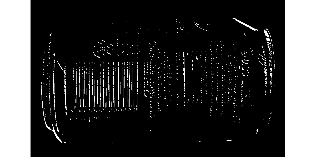
   Figure 11.9 – Binary output

6. As shown in the preceding image, it is a binary image with the barcode and other high vertical gradient areas highlighted. We can dilate the image for further processing. It fills in the gap in between the vertical lines:

   dilated = cv2.dilate(th, None, iterations = 10)

   The output of the preceding code contains a lot of rectangle-shaped boxes corresponding to the barcode and other regions in the original image. We are interested in the region containing the barcode, not the other regions:

   

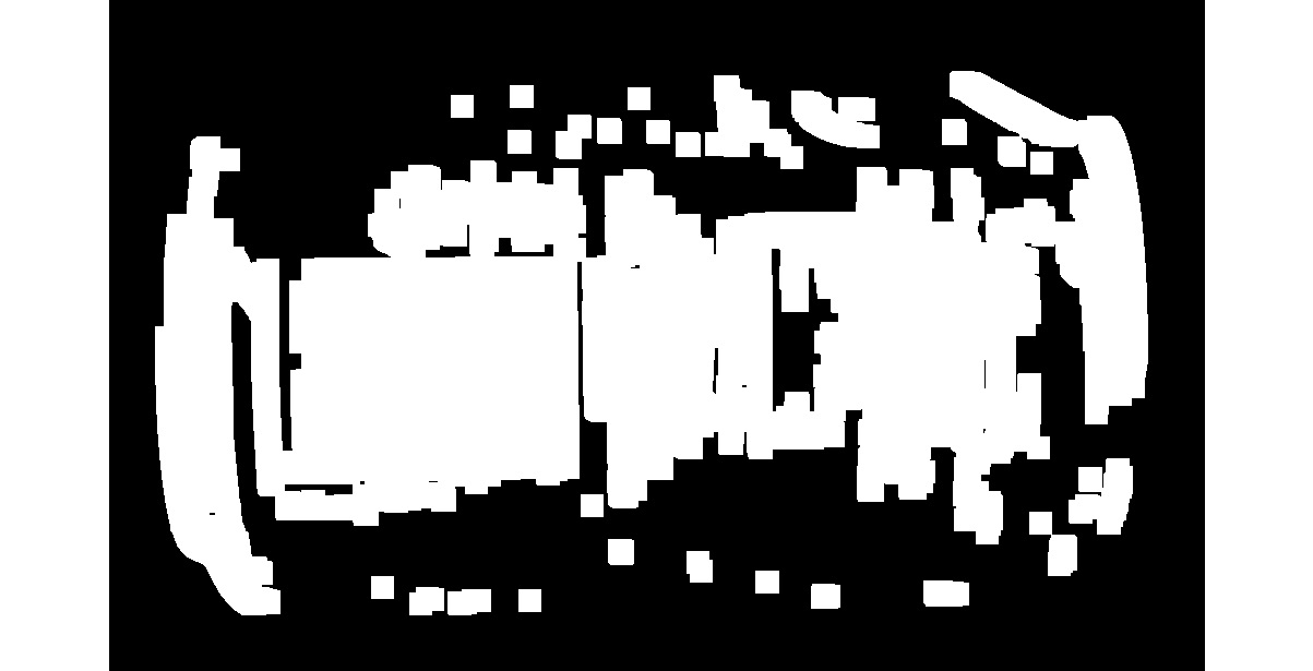
   Figure 11.10 – Dilated binary output

7. The morphological erosion operation will eliminate most of the other regions that do not correspond to the barcode:

   eroded = cv2.erode(dilated, None, iterations = 15)

   The following is the output of the preceding code:

   

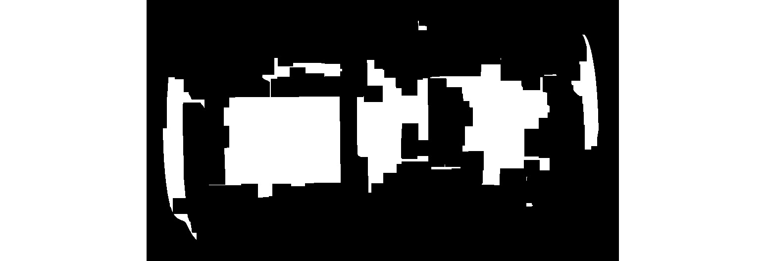
   Fig.11.11 – Eroded image

8. Let's find the list of all the contours in this computed binary image. Use the following code to do so:

   (contours, hierarchy) = cv2.findContours(eroded, cv2.RETR_TREE, cv2.CHAIN_APPROX_SIMPLE)

9. The biggest contour in this binary image is the contour corresponding to the region of the barcode. The following code finds the biggest contour in the image:

   areas = [cv2.contourArea(temp) for temp in contours]

   max_index = np.argmax(areas)

   largest_contour = contours[max_index]

10. Let's retrieve the coordinates of the bounding rectangle of the biggest contour with the OpenCV cv2.boundingRect() function and then draw the rectangle in the image:

    x, y, width, height = cv2.boundingRect(largest_contour)

    cv2.rectangle(image, (x, y), (x+width, y+height),(0,255,0), 2)

    cv2.imshow('Detected Barcode',image)

    cv2.waitKey(0)

    cv2.destroyAllWindows()

    The preceding code draws the bounding rectangle over the area corresponding to the biggest contour in the image (which is the region of the barcode), as shown in the following output:

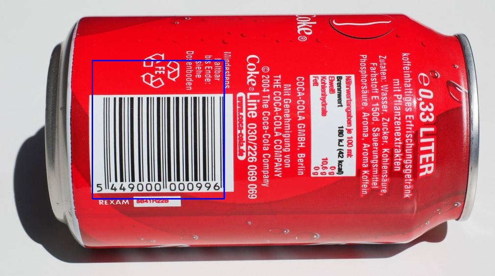
Figure 11.12 – Detected barcode

As shown in the previous screenshot, the approximate region with the barcode is outlined with a blue colored rectangle. This same code may not work with a lot of images, but it works with most images. We may have to tune the code to detect the regions with barcodes in the other images. You might want to change the following lines of code for the specific inputs:

blur = cv2.GaussianBlur(diff, (3, 3), 0)

dilated = cv2.dilate(th, None, iterations = 10)

eroded = cv2.erode(dilated, None, iterations = 15)

Based on this program, we can create many real-life applications. The first application is a barcode region detector for a live video feed from a USB webcam. The other application we can create is a generic program to detect barcodes. To tune the arguments that are passed to the functions, we can use trackbars.

In the next section, we will learn how to apply film-style chroma keying with OpenCV and Python 3 using the RPi and a USB webcam.

Implementing the chroma key effect

Chroma keying is also known as chroma key compositing. It is also colloquially known as the green screen or blue screen effect due to the green or blue background that we use while creating this effect. It is a post-production technique and can also be used on still images and live videos. In the chroma key effect, we place an object or a person in the foreground and capture an image or footage. The background is usually a green- or blue-colored fabric or wall. Then, we replace the green or blue color in the captured image or footage with another video or an image. This makes the viewers feel that the person or the object in the foreground is at a different location than the studio where they were filmed. This effect is one of the most used effects in film-making and live weather forecasts in news broadcasts:

1. Let's start by importing all the needed libraries and initiating a video capture object:

   import numpy as np

   import cv2

   cap = cv2.VideoCapture(0)

2. To obtain the better frame rate or frames per second (FPS), let's set the resolution of the USB webcam to 640x480 pixels. This will yield a better frame rate and the green screen effect will look natural:

   cap.set(3, 640)

   cap.set(4, 480)

3. In the next step, we read the image that is to be used as the background. The image to be used as the background must have the same resolution as the resolution the webcam is set to. In this case, we have set it to 640x480. We know that all the arithmetic and logical operations that we will perform on NumPy arrays (in this case, the background image and the frames of the live feed from the USB webcam connected to the RPi) need the operand arrays to be of the same dimensions; otherwise, the Python 3 interpreter will throw an error. The following is the code for this:

   bg = cv2.imread('/home/pi/book/dataset/bg.jpg', 1)

4. Let's write the familiar logic for the loop and read the frames of the live feed from the USB webcam, as follows:

   while True:

   ret, frame = cap.read()

   We can use a green colored cloth (such as a curtain) or paper as the background for this demonstration. We will also use the box of the RPi camera module as the object in the foreground. The following is a photo of the original scene:

   

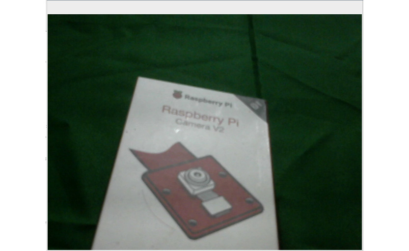
   Figure 11.13 – Input video

5. As we discussed in Chapter 6, Colorspaces, Transformations, and Thresholding, when we need to work with color ranges, the HSV colorspace is the best way to represent colors. Let's convert the image into the HSV colorspace and then compute the mask for the green screen in the background with the following code:

   hsv=cv2.cvtColor(frame, cv2.COLOR_BGR2HSV)

   image_mask=cv2.inRange(hsv, np.array([40, 50, 50]),

   np.array([80, 255, 255]))

   This computes the mask for the image. The pixels in green (or any shade of it) are replaced with color and the remaining pixels are replaced with black:

   

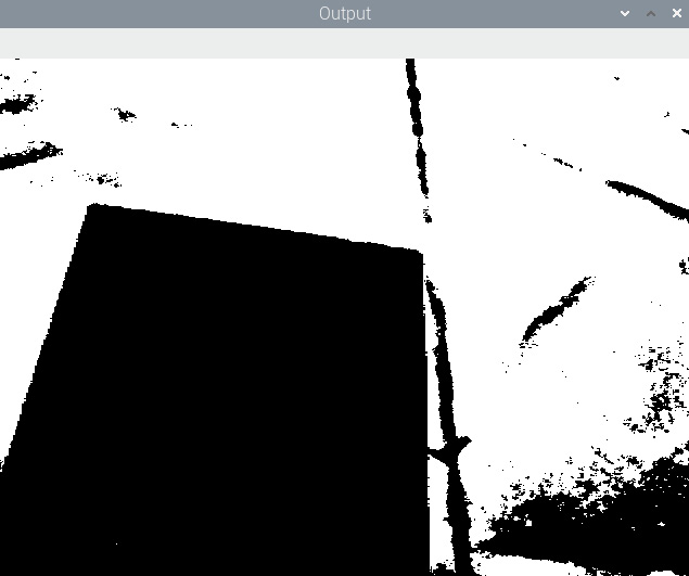
   Figure 11.14 – Computing the mask

6. After computing the mask corresponding to the background image, we can apply the mask to the image in the background in order to hide the object in the foreground with the black pixels, as follows:

   bg_mask=cv2.bitwise_and(bg, bg, mask=image_mask)

   The preceding code replaces the white pixels with the pixels of the image we chose as the background. Also, the pixels corresponding to the foreground are in black, as shown in the following output:

   

   Figure 11.15 – White pixels in the mask replaced with the background

7. Now, we must extract the foreground from the live feed of the USB webcam. We can do this with the following code:

   fg_mask=cv2.bitwise_and(frame, frame, mask=cv2.bitwise_not(image_mask))

   The preceding code extracts all the pixels that are not green (or shades of it). It also assigns the color black to the pixels that correspond to the background (the green screen):

   

   Figure 11.16 – Black pixels in the mask replaced with the foreground

8. Now, it is time for us to add the last two outputs we computed. This will replace the green background with the custom image and produce the chroma key effect:

   cv2.imshow('Output', cv2.add(bg_mask, fg_mask))

   if cv2.waitKey(1) == 27:

   break

   cv2.destroyAllWindows()

   cap.release()

   The following is the final output:

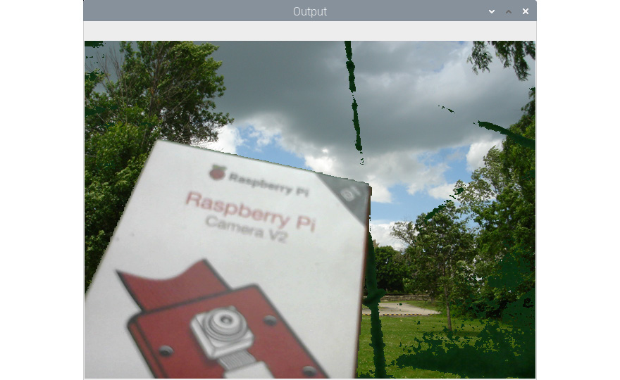
Figure 11.17 – Final output

Congratulations! We have managed to achieve a film-style chroma key effect with our RPi camera module box and a green cloth. We can see that the effect is imperfect. This is due to imperfect illumination. The webcam is not registering a few pixels as green pixels, but pixels of another color. The remedy to this is to have good and uniform illumination for the green background and foreground object.

The simple rule to be followed while implementing the chroma key effect is that the object we are chroma keying must not be the same color as the background screen. So, if we are using a green colored background, then neither the object nor any of its part can be green. The same is true for a blue background screen.

Summary

In this chapter, have learned how to demonstrate real-life applications using the concepts and techniques in computer vision we learned about in the previous chapters of this book. With the concepts we learned in this chapter, we can write a program for creating a simple security application.

From here on out, using the knowledge we've gained from the experiments in this book, we can explore the areas of image processing and computer vision with OpenCV in more detail. Our journey surrounding the OpenCV library concludes here.

In the next chapter, we will learn how to use another powerful, yet very easy to use, computer vision library for Python called Mahotas. We will also learn and demonstrate how to use Jupyter Notebook for scientific programming with Python 3.