Chapter 3: Introduction to Python Programming

In the previous chapter, we learned how to remotely access the Command Prompt and the desktop of a Raspberry Pi (RPi) board. We also installed OpenCV for Python 3. Finally, we learned how to overclock the RPi and examined the various heatsinks for the RPi.

Continuing from where we left off at the end of the previous chapter, in this chapter, we will start by looking at Python 3 programming on the RPi. We will have a brief look at the Scientific Python (SciPy) ecosystem and all the libraries in it. Then, we will write basic programs for numerical computation with NumPy N-Dimensional Arrays (ndarrays). We will also learn how to visualize data with Matplotlib. Finally, we will explore the hardware aspects of the RPi with the General Purpose Input Output (GPIO) library of Python for the RPi.

In short, we will cover the following topics:

• Understanding Python 3
• The SciPy ecosystem
• Programming with NumPy and Matplotlib
• RPi GPIO programming

Technical requirements

The code files of this chapter can be found on GitHub at https://github.com/PacktPublishing/raspberry-pi-computer-vision-programming/tree/master/Chapter03/programs.

Check out the following video to see the Code in Action at https://bit.ly/37UVwmO.

Understanding Python 3

Python is a high-level, interpreted, general-purpose programming language. It was created by Guido van Rossum and was started as a personal hobby project but has since grown into what it is today. The following is a timeline of the major milestones in the development of the Python programming language:

Figure 3.1 – Timeline of Python development milestones

Guido van Rossum held the title of benevolent dictator for life for the Python project for most of its life cycle. He stepped down from the role in July 2018 and has been part of the Python Steering Council ever since.

You can read more about Python on its home page at www.python.org.

The Python programming language has two major versions—Python 2 and Python 3. They are mostly incompatible with one another. As the preceding timeline shows, Python 2's sunset happened on 31st December 2019. This means that there is no further development of Python 2. Official support has also ceased to exist. The only Python version under active development and with continued support is Python 3. A lot of code (in fact, billions of lines of code) that is in production for many organizations is still in Python 2. So, the migration from Python 2 to Python 3 requires a major effort.

Python on RPi and Raspberry Pi OS

Python comes pre-installed on the Raspberry Pi OS image that we downloaded. Both versions of Python—Python 2 and Python 3—come with the Raspberry Pi OS image. We will look at Python 3 in detail as we will write all of our programs with Python 3.

Open lxterminal or log in remotely to the RPi and run the following command:

python -V

This produces the following output:

Python 2.7.16

The -V option returns the version of the Python interpreter. So, the python command refers to the Python 2 interpreter. However, we need Python 3. So, run the following command in the Command Prompt:

Python3 -V

This produces the following output:

Python 3.7.3

This is the Python 3 interpreter and we will use it for all of our programming exercises throughout this book. To find out the location of the interpreter on your disc (in our case, our microSD card), run the following command:

which python3

This produces the following output:

/usr/bin/python3

This is where the executable for the Python 3 interpreter is located.

Python 3 IDEs on Raspberry Pi OS

Before we get started with Python 3 programming, we will learn which Integrated Development Environments (IDEs) can be used to write programs with Python. Raspberry Pi OS, as of now, comes with two IDEs. Both can be accessed from the Programming option in the Raspbian menu, as shown:

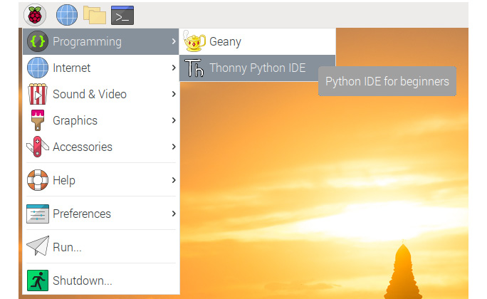
Figure 3.2 – The Thonny and Geany Python IDEs in the Raspbian menu

The first option is the Geany IDE, which can be used with many programming and markup languages, including Python 2 and Python 3. You can read more about it at https://geany.org/. The second option is Thonny Python IDE, which supports Python 3 and the MicroPython variants.

I personally prefer to use Integrated Development and Learning Environment (IDLE), which is developed and maintained by the Python Foundation. You can read more about it at https://docs.python.org/3/library/idle.html. Earlier versions of Raspberry Pi OS used to come with IDLE. However, it is no longer present in the latest version of Raspberry Pi OS. Instead, we have Geany and Thonny. However, we can download IDLE with the following command:

sudo apt-get install idle3 -y

Once installed, we can find it in the Programming menu option under the Raspbian menu, as shown in the following screenshot:

Figure 3.3 – The option for IDLE for Python 3

Click on it to open it. Alternatively, we can launch it from the Command Prompt with the following command:

idle

Note that this command will not work and will throw an error if we have remotely connected to the Command Prompt of the RPi (using an SSH client such as PuTTY or Bitvise) as the command invokes the GUI. It will work if a visual display is directly connected to the RPi or if we access the RPi desktop remotely. This invokes a new window, as follows:

Figure 3.4 – Python 3 interactive mode in IDLE

This is the Python 3 interpreter prompt, or Python 3 shell. We will discuss this concept in detail later in this chapter.

Now, go to File | New File from the top menu. This will open a new code editor window, as follows:

Figure 3.5 – A new blank Python program

The interpreter window will also stay open when this happens. You can either close or minimize it. If you find it difficult to read the text in the interpreter or code editor in IDLE due to the size of the font, you can go to Options | Configure IDLE from the menu to set the font and size of the text. The configuration window looks as follows:

Figure 3.6 – IDLE configuration

Let's write a customary Hello World! program. Type the following text into the window:

print('Hello World!')

Then, from the menu, click Run | Run Module. It will ask you to save it. Click the OK button and it will take you to the Save dialog box. I prefer to save the code for this book by chapter in a directory, with sub-directories for each chapter. You can make the directory structure by running the following commands in the home directory of the pi user:

mkdir book

mkdir book/dataset

mkdir book/chapter01

We can make a separate directory for each chapter like this. Also, a separate dataset directory to store our data is needed. After creating the prescribed directory structure, run the following sequence of commands:

cd book

tree

We can see the directory structure in the following output of the tree command:

Figure 3.7 – Directory structure for saving programs for this book

We can create the same directory structure by using the Save dialog box of IDLE or the File Manager application of Raspberry Pi OS.

Once the directory corresponding to the current chapter is created, save the file there as prog00.py. You just need to enter the filename; IDLE will automatically assign the .py extension to the file. Then, the file will be executed by the Python 3 interpreter and the output will be visible in the interpreter shell, as follows:

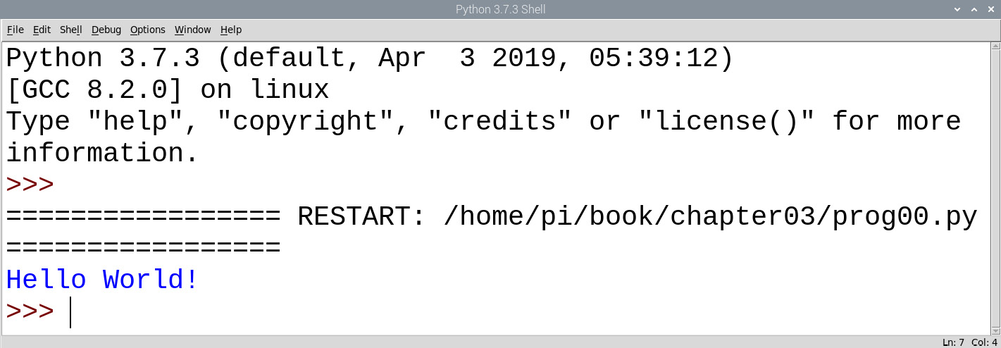
Figure 3.8 – Execution of a Python 3 program in IDLE

We can also write the same code with the Nano editor. The only difference is that we also need to provide an extension when saving it. We can navigate to the directory that has the prog00.py file and run the following command to feed the file to the Python 3 interpreter:

python3 prog00.py

The Python 3 interpreter will execute the program and print the output, as follows:

Figure 3.9 – Execution of a Python 3 program in LXTerminal

Working with Python 3 in interactive mode

We have seen how to write a Python 3 program using the IDLE and Nano editors. We have also seen how to launch the program using IDLE and from the Command Prompt of Raspberry Pi OS. Running a Python 3 program in this fashion is known as script mode.

There is also another mode—interactive mode. In interactive mode, we launch the Python interpreter and it acts as a command-line interpreter. When we enter and run a statement, we get immediate feedback from the interpreter. We can launch the interactive mode in two ways. We have already seen the first way. When we launch IDLE, it opens the interpreter and we can use it to run the Python 3 statements. The other way is to run the python3 command in the Command Prompt. This will invoke the Python 3 interpreter in the Command Prompt, as follows:

Figure 3.10 – Python 3 in interactive mode on the Command Prompt

Type the following statement into the prompt:

>>> print('Hello World!')

Then, press Enter. It will be executed and the output will be shown on the next line. This way, we can execute single-line statements and small code snippets like this. We will be using interactive mode extensively in this chapter. From the next chapter onward, we will use script mode—that is, we will save the programs in files and launch them from the command prompt or IDLE.

The basics of Python 3 programming

Let's start by learning the basics of Python 3 programming. Open the Python 3 interactive prompt. Type in the following statements:

>>> pi = 3.14

>>> print(pi)

This will show the value of the pi variable. Run the following statement:

>>> print(type(3.14))

This shows the following output:

<class 'float'>

You might have noticed that we have not declared the data type of the variable here. That is because Python is a dynamically typed programming language. We also say that the variable belongs to a class type. This means that it is an object, which is true for all variables and other constructs in Python. Everything is an object in Python. This makes Python a truly object-oriented programming language. Almost everything has attributes and methods.

In order to exit the Command Prompt, press Ctrl + D or run the exit() statement.

Let's create our own class and an object of that class. Save the file and name it prog01.py, then add the following code to it:

class Person:

def __init__(self, name='', age=0):

self.name = name

self.age = age

def show(self):

print(self.name)

print(self.age)

In the preceding code, we defined Person. The __init__() class is the initializer function and it is called automatically whenever an object of the Person class is created. The self parameter is a reference to the current instance of the class and is used to access variables that belong to the class within the class definition.

Let's add some more code to prog01.py. We will create a class object, as follows:

p1 = Person('Ashwin', 25)

p1.show()

We created the p1 class and then showed the properties of the object with the show() function call. Here, we are assigning the values to class member variables at the time of the creation of the class object.

Let's look at another way to create an object and assign values to the member variables. Add the following code to the file:

p2 = Person()

p2.name = 'Jane'

p2.age = 20

print(p2.name)

print(p2.age)

In the preceding code, we are creating an object and the initializer function is called with the default arguments. Then, we are assigning the values to the class variables and accessing them directly using the class object. Run the program and see the output.

Now, open the Python 3 interpreter and run the following statements:

>>> import sys

>>> print(sys.platform)

This will return the name of the current OS (Linux). The first statement imports sys, which is a Python standard library. It comes with the Python interpreter as part of its batteries included motto. This means the Python interpreter comes with a large set of useful libraries. sys.platform returns the current OS name string.

Let's try another example. In the previous chapter, we installed the OpenCV library. Let's import that again now. We have already tested it directly from the Raspberry Pi OS Command Prompt. Let's try to do the same in interactive mode:

>>> import cv2

>>> print(cv2.__version__)

The first statement imports the OpenCV library to the current session. The second statement returns a string that contains the version number of the installed OpenCV library.

There are many topics in the basics of Python 3 programming, but it is very difficult to cover all of them. Also, to do so is beyond the scope of this book. However, we will use the topics we have just learned quite frequently in this book.

In the next section, we will explore the SciPy ecosystem libraries.

The SciPy ecosystem

The SciPy ecosystem is a collection of libraries for programming science, mathematics, and engineering functionalities. It has the following libraries as core components:

• NumPy
• SciPy
• Matplotlib
• IPython
• SymPy
• pandas

In this book, we will use all of these libraries except SymPy and pandas. In this section, we will have a look at the NumPy and Matplotlib libraries. We will learn the useful aspects of the other two libraries in the later chapters of this book.

The basics of NumPy

NumPy is a fundamental package that can be used for numerical computation with Python. It is a matrix library for linear algebra. NumPy ndarrays can also be used as an efficient multi-dimensional container of generic data. Arbitrary data types can also be defined and used. NumPy is an extension of the Python programming language. It adds support for large multi-dimensional arrays and matrices, along with a large library of high-level mathematical functions that can be used to operate on these arrays. We will use NumPy arrays throughout this book to represent images and carry out complex mathematical operations. NumPy comes with many built-in functions for all of these operations. So, we do not have to worry about basic array operations. We can focus directly on the concepts and code for computer vision. All of the OpenCV array structures are converted to and from NumPy arrays. So, whatever operations you perform in NumPy, you can always combine NumPy with OpenCV.

We will use NumPy with OpenCV a lot in this book. Let's start with some simple example programs that will demonstrate the real power of NumPy.

NumPy comes pre-installed on Raspberry Pi OS. So, we do not have to install it separately.

Open the Python 3 interpreter and try the following examples.

Creation of ndarrays

Let's see some examples on ndarray creation. The array() method will be used very frequently in this book. There are many ways to create different types of arrays. We will explore these methods as and when they are needed in this book. Follow these commands for ndarray creation:

>>> import numpy as np

>>> x=np.array([1,2,3])

>>> x

array([1, 2, 3])

>>> y=arange(10)

>>> y=np.arange(10)

>>> y

array([0, 1, 2, 3, 4, 5, 6, 7, 8, 9])

Basic operations on ndarrays

We are going to learn about the linspace() function now. It takes three parameters—start_num, end_num, and count. This creates an array with equally spaced points, starting from start_num and ending with end_num. You can try out the following example:

>>> y=np.arange(10)

>>> y

array([0, 1, 2, 3, 4, 5, 6, 7, 8, 9])

>>> a=np.array([1,3,6,9])

>>> a

array([1, 3, 6, 9])

>>> b=np.linspace(0,15,4)

>>> b

array([ 0., 5., 10., 15.])

>>> c = a - b

>>> c

array([ 1., -2., -4., -6.])

The following is the code that can be used to calculate the square of every element in an array:

>>> a**2

array([ 1, 9, 36, 81], dtype=int32)

Linear algebra with ndarrays

Let's explore some examples relating to linear algebra. You will learn how to use the transpose(), inv(), solve(), and dot() functions, which are useful when performing operations related to linear algebra:

>>> a = np.array([[1,2,3],[4,5,6],[7,8,9]])

>>> a.transpose()

array([[1, 4, 7],

[2, 5, 8],

[3, 6, 9]])

>>> np.linalg.inv(a)

array([[-4.50359963e+15, 9.00719925e+15, -4.50359963e+15],

[ 9.00719925e+15, -1.80143985e+16, 9.00719925e+15],

[-4.50359963e+15, 9.00719925e+15, -4.50359963e+15]])

>>> b = np.array([3, 2, 1])

>>> np.linalg.solve(a, b)

array([-9.66666667, 15.33333333, -6. ])

>>> c = np.random.rand(3, 3)

>>> c

array([[0.91827923, 0.75063499, 0.40049332],

[0.09520566, 0.16718726, 0.6577751 ],

[0.95343917, 0.50972786, 0.65649385]])

>>> np.dot(a, c)

array([[ 3.96900804, 2.61419309, 3.68552507],

[ 9.86978019, 6.89684344, 8.82981189],

[15.77055234, 11.17949379, 13.9740987 ]])

Note:

You can explore NumPy in more detail at http://www.numpy.org.

Matplotlib

Matplotlib is a plotting library for Python and it produces publication-quality figures. It can produce various types of visualizations, such as plots, three-dimensional visualizations, and images. It is important to understand the basics of Matplotlib to work with any computer vision library, such as OpenCV.

Matplotlib was developed by John D. Hunter and it is continually developed by the open source community. It is an integral part of the SciPy ecosystem. All the other libraries in the SciPy ecosystem use Matplotlib for the visualization of data. pyplot is a module in Matplotlib that provides a MATLAB-like interface for the visualization of data.

Before we begin programming with Matplotlib, we need to install it as it does not come pre-installed on Raspberry Pi OS.

We can install it with the pip3 utility. We have already seen how to use this utility when installing OpenCV. Let's look at it in more detail. pip means Pip Installs Packages or Pip Installs Python. It is a recursive acronym (meaning the acronym is itself part of the acronym). It is a command-line utility that comes with the Python interpreter and is used for installing libraries. pip3 is the Python 3 version of this utility. It first connects to the Python Package Index, which is a repository of Python libraries. Then, it downloads and installs the library we need.

Note:

You can read more about the Python Package Index and pip at https://pypi.org/project/pip/ and https://pypi.org/.

We can install Matplotlib by running the following command:

pip3 install matplotlib

Matplotlib is a big library and has many prerequisite libraries. All of these prerequisite libraries are automatically installed by pip3 and then Matplotlib is installed. It will take some time to do so, depending on the speed of your internet connection.

Once the installation is complete, we can write a few sample programs. We will use Python 3 in script mode and IDLE or the Nano editor to write programs. Create a new file, prog02.py, and add the following code to it:

import matplotlib.pyplot as plt

import numpy as np

x = np.array([1, 2, 3, 4], dtype=np.uint8)

y = x**2 + 1

plt.plot(x, y)

plt.grid('on')

plt.show()

In the first line of the preceding code, we import Matplotlib's pyplot module with the plt alias. Then, we import NumPy. We use the array() function call to create a linear ndarray by passing it a list of 8-bit unsigned integers (uint8 refers to the data type). Then, we define y = x2 + 1. The plot() function plots y versus x. We can set the grid on or off by passing 'on' or 'off' to the grid() function call. The show() function call starts an event loop, looks for all the currently active visualization objects, and opens a visualization window to show the plots or the other visualization. The following is the output:

Figure 3.11 – Visualization with Matplotlib

As we can see, this shows us the visualization. The grid is visible as we turned it on. We also have image controls at the bottom where we can save, zoom, and perform other operations on the visualization. Note that we need to run the program directly on the RPi by using IDLE on the Command Prompt or by using the remote desktop. Running the program from a remote SSH command line will not throw any error but it won't show any output either.

Save the prog02.py code file as prog03.py. After the plot() function call and before grid() call, add the following lines:

y = x + 1

plt.plot(x, y)

plt.title('Graph')

plt.xlabel('X-Axis')

plt.ylabel('Y-Axis')

The rest of the code remains as it is. Save the program. Here, we are demonstrating the visualization of multiple plots in the same window. We are also adding a title and labels to the graph. Run the prog03.py file and the following is the output:

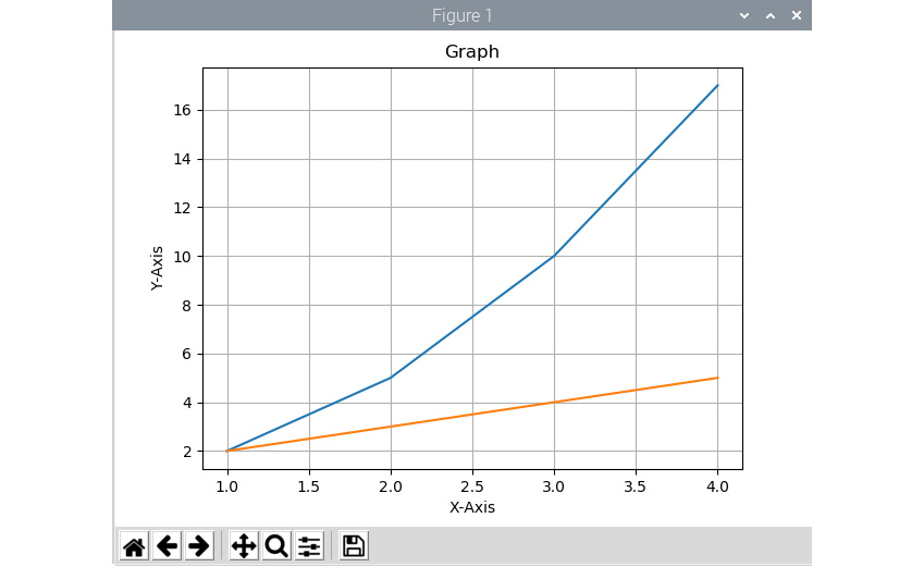
Figure 3.12 – Multiple graphs with Matplotlib

We can add the following line just before plt.show() to save the visualization on the disk:

plt.savefig('test1.png', dpi=300, bbox_inches='tight')

This will save the visualization in the current directory and name it test1.png.

Let's move on to the more interesting part. We can visualize ndarrays as images with the imshow() function. Let's see an example. Create a new file named prog04.py and add the following code to it:

import matplotlib.pyplot as plt

import numpy as np

x = np.array([[0, 1, 2, 3, 4],

[5, 6, 7, 8, 9]], dtype = np.uint8 )

plt.imshow(x)

plt.show()

In the preceding code, we are creating a two-dimensional array (with a size of 5x2) and visualizing it as an image with the imshow() call. The following is the output:

Figure 3.13 – Visualizing numbers as an image

As this is an image, we really do not need grid and axis ticks. We can add the following two lines to the code before plt.show() to turn them off:

plt.axis('off')

plt.grid('off')

Run the modified code and observe the output.

The image has been rendered with what we call as default colormap. A colormap is a color scheme for visualizations. If we change plt.imshow(x) to plt.imshow(x, cmap='gray'), then the following is the output:

Figure 3.14 – The image in greyscale mode

There are a lot of colormaps. We can even create our own custom colormaps; however, for the demonstration of computer vision algorithms, that is not needed as the existing colormaps suffice. If you are curious about the available colormap names that we can use, you can find them out as follows. Open the Python 3 interpreter in the interactive mode and import the pyplot module to Matplotlib:

>>> import matplotlib.pyplot as plt

The plt.colormaps() list has names of all the colormaps. First, we check how many colormaps are there, which is easy. Run the following statement:

>>> print(len(plt.colormaps()))

This will print the number of colormaps. Finally, run the following statement to see a list of all the available colormaps:

>>> print(plt.colormaps())

The list is quite long and we will be using only a few of the colormaps from the list for our demonstrations. In the prog04.py file, change plt.imshow(x) to plt.imshow(x, cmap='Accent'), and the following will be the output:

Figure 3.14 – The image with the Accent colormap

This much knowledge of Matplotlib is more than enough to get started with OpenCV and computer vision.

Up to now, we have seen examples of visualization of one-dimensional and two-dimensional ndarrays. Now, let's see how we can create a random three-dimensional ndarray and how to visualize it. Observe the following code:

import matplotlib.pyplot as plt

import numpy as np

x = np.random.rand(3, 3, 3)

plt.imshow(x)

plt.axis('off')

plt.grid('off')

plt.show()

In the preceding code, we are using np.random.rand() to create a random three-dimensional array. We just need to pass to it the size of every dimension. In the preceding example, we are creating a three-dimensional matrix with a size of 3x3x3. Run the preceding code and see the output for yourself. All the images we will work with throughout this book are represented as either two-dimensional or three-dimensional ndarrays. This knowledge of data visualization will be very helpful once we start working with images.

RPi GPIO programming with Python 3

One of the main unique selling points of the RPi and similar single-board computers is the onboard GPIO pins. A few early models of the RPi boards have 26 pins. Most recent models have 40 pins for GPIO. We can obtain the details of the pins on a board by running the pinout command on the Command Prompt. The following is the output of the command for my RPi 4B board:

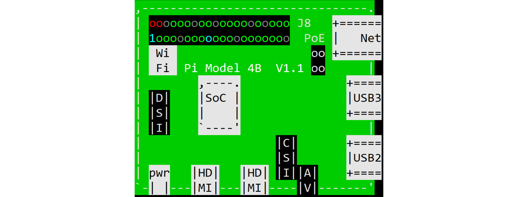
Figure 3.16 – Part 1 of the command pinout

In the top left, we can see the 40 pins for GPIO. Pin number 1 is labeled there. The red circle above it is pin number 2. The pin adjacent to pin number 1 is pin number 3, and so on. The following part of the output shows the numbering of all the pins:

Figure 3.17 – Part 2 of the command pinout

As we can see in the preceding output, we have power pins (3V3, 5V, and GND) and digital I/O pins, marked as GPIOxx.

LED programming with GPIO

Now, we will see how to program LEDs with GPIO pins as output pins. Let's prepare a simple circuit for blinking an LED, first.

For that, we need jumper cables, an LED, and a 220-ohm resistor. Prepare your circuit as in the following diagram:

Figure 3.18 – LED-resistor circuit

As we can see in the preceding circuit diagram, we are connecting the anode of the LED to physical pin 8 through a 220-ohm resistor, and the cathode of the LED is connected to physical pin 6, which is a Ground (GND) pin.

Note:

You will find many beautiful circuit diagrams like this throughout this book. I used an open source software called Fritzing to generate them. You can access Fritzing's home page at https://fritzing.org/. Fritzing files have the *.fzz extension. These files are part of the downloadable code bundle for this book.

Now, let's get into the code. For that, we need to install the GPIO library. The latest version of Raspberry Pi OS comes with the GPIO library already installed. However, if it is not there, we can install it by running the following command:

sudo apt-get install python3-rpi.gpio -y

Now, create a new file, prog05.py, in the same directory and add the following code to it:

import RPi.GPIO as GPIO

from time import sleep

GPIO.setwarnings(False)

GPIO.setmode(GPIO.BOARD)

GPIO.setup(8, GPIO.OUT, initial=GPIO.LOW)

while True:

GPIO.output(8, GPIO.HIGH)

sleep(1)

GPIO.output(8, GPIO.LOW)

sleep(1)

In the preceding code, the first two lines import the required libraries. setwarnings(False) disables all the warnings and setmode() is used to set the pin addressing mode. There are two modes, GPIO.BOARD and GPIO.BCM. In the GPIO.BOARD mode, we refer to the pins by their physical location numbers. In the GPIO.BCM mode, we refer to the pins by their Broadcom SOC channel number. I prefer the GPIO.BOARD mode because it is easy to remember the pins by their physical location number. setup() is used to set each GPIO pin as an input or output.

In the preceding code, the first argument is the pin number, the second argument is the mode, and the third one is the initial state of the pin. output() is used to send either HIGH or LOW signals to the pin. sleep() is imported from the time library and it produces a delay of a given number of seconds. Run the preceding program to make the LED blink. In order to terminate the program, press Ctrl + C on the keyboard.

Similarly, we can write the following code for the same circuit to flash the LED to convey a Save our Souls (SOS) message visually:

import RPi.GPIO as GPIO

from time import sleep

GPIO.setwarnings(False) # Ignore Warnings

GPIO.setmode(GPIO.BOARD) # Use Physical Pin Numbering

GPIO.setup(8, GPIO.OUT, initial=GPIO.LOW)

def flash(led, duration):

GPIO.output(led, GPIO.HIGH)

sleep(duration)

GPIO.output(led, GPIO.LOW)

sleep(duration)

while True:

flash(8, 0.2)

flash(8, 0.2)

flash(8, 0.2)

sleep(0.3)

flash(8, 0.5)

flash(8, 0.5)

flash(8, 0.5)

flash(8, 0.2)

flash(8, 0.2)

flash(8, 0.2)

sleep(1)

In the preceding program, we defined a custom flash() function that accepts the pin number and the duration of the flash. Then, we set the provided pin to HIGH for the given duration and then set it to LOW for the given duration. So, the LED connected to the pin is alternately turned on and off for the given duration. When this happens in the pattern of . . . - - - . . . (triple dots followed by a triple dash followed by triple dots), which is Morse code for SOS, it is called a distress signal. For each . (dot) character, we flash the LED for 0.2 seconds, and for each – (dash) character, we flash it for half a second. We have added all of this to the preceding infinite while loop. When we run the program, it starts flashing the SOS message until we terminate it by pressing Ctrl + C on the keyboard.

Let's look at some more GPIO and Python 3 programming. Prepare a circuit as in the following diagram:

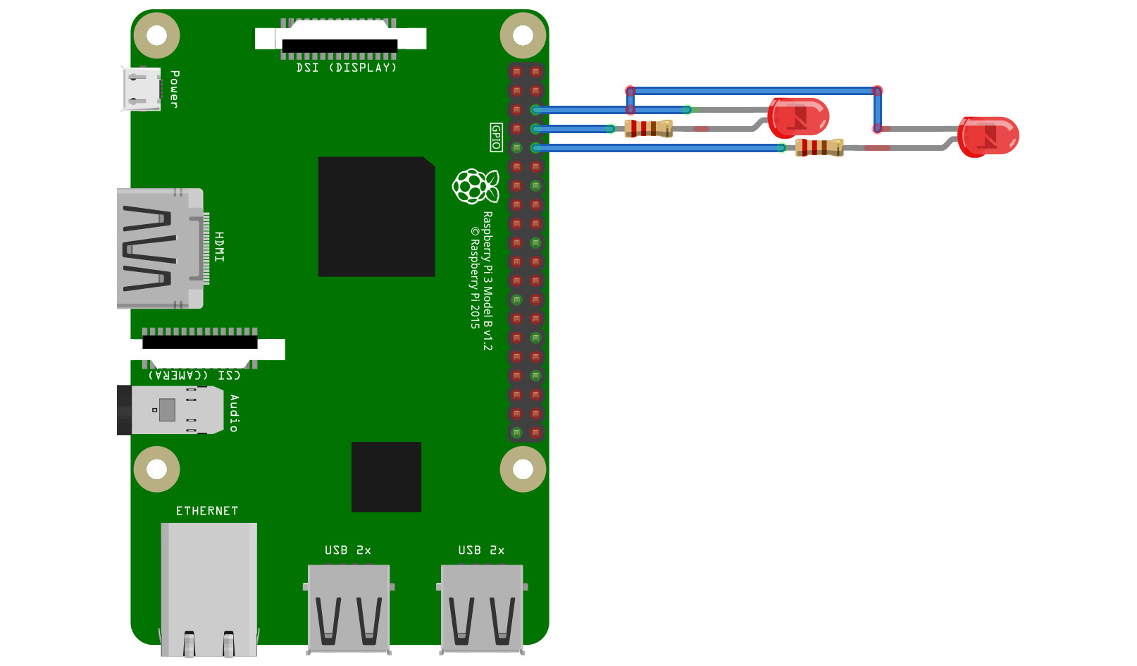
Figure 3.19 – A circuit diagram with two LEDs

As we can see here, we just need to connect the anode of an additional LED to pin 10 through a 220-ohm resistor and a cathode of the same LED to the GND pin. We will make both the LEDs blink alternately. The following is the code for this:

import RPi.GPIO as GPIO

from time import sleep

GPIO.setwarnings(False)

GPIO.setmode(GPIO.BOARD)

GPIO.setup(8, GPIO.OUT, initial=GPIO.LOW)

GPIO.setup(10, GPIO.OUT, initial=GPIO.LOW)

while True:

GPIO.output(8, GPIO.HIGH)

GPIO.output(10, GPIO.LOW)

sleep(1)

GPIO.output(8, GPIO.LOW)

GPIO.output(10, GPIO.HIGH)

sleep(1)

You should now be familiar with all of the functions in the preceding code as we discussed them in the earlier two examples. This code, upon execution, makes the LEDs blink for 1 second alternately.

Now, there is another way to produce the same output. Take a look at the following program:

import RPi.GPIO as GPIO

from time import sleep

GPIO.setwarnings(False)

GPIO.setmode(GPIO.BOARD)

GPIO.setup(8, GPIO.OUT, initial=GPIO.LOW)

GPIO.setup(10, GPIO.OUT, initial=GPIO.LOW)

counter = 0

while True:

if counter % 2 == 0:

led1 = 8

led2 = 10

else:

led1 = 10

led2 = 8

GPIO.output(led1, GPIO.HIGH)

GPIO.output(led2, GPIO.LOW)

sleep(1)

counter = counter + 1

In the preceding program, we are using slightly different logic to demonstrate the usage of if statement in Python 3. We have a variable named counter, which is set to 0 at the beginning. In the while loop, we check whether the counter value is even or odd, and depending on that, we set which LED is to be turned on and which is to be turned off. At the end of the loop, we increment counter by 1. The output of this program is the same as the earlier one and it can be terminated by pressing Ctrl + C.

Now, let's experiment with numerous LEDs. We will need a breadboard for this. Prepare a circuit as in the following diagram:

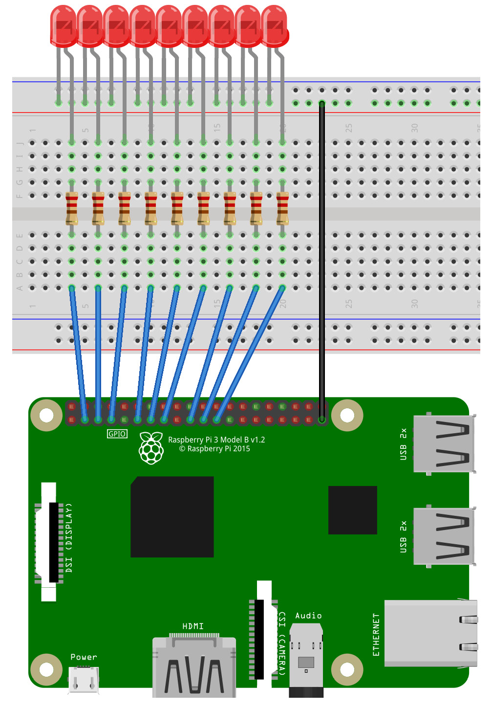
Figure 3.20 – A diagram for the chaser circuit

For programming, we will try a bit of a different approach. We will use the gpiozero library of Python 3. If it is not installed by default on your Raspbian distribution, it can be installed with the following command:

pip3 install gpiozero

This uses the BCM numbering system when addressing the pins. Save the following code in a Python file and run it to see a beautiful chaser effect:

from gpiozero import LED

from time import sleep

led1 = LED(2)

led2 = LED(3)

led3 = LED(4)

led4 = LED(17)

led5 = LED(27)

led6 = LED(22)

led7 = LED(10)

led8 = LED(9)

led9 = LED(11)

sleeptime = 0.2

while True:

led1.on()

sleep(sleeptime)

led1.off()

led2.on()

sleep(sleeptime)

led2.off()

led3.on()

sleep(sleeptime)

led3.off()

led4.on()

sleep(sleeptime)

led4.off()

led5.on()

sleep(sleeptime)

led5.off()

led6.on()

sleep(sleeptime)

led6.off()

led7.on()

sleep(sleeptime)

led7.off()

led8.on()

sleep(sleeptime)

led8.off()

led9.on()

sleep(sleeptime)

led9.off()

All of the preceding code is self-explanatory and should be easy for you to understand by now. In the first line, we imported LED. We can pass to it a BCM pin number as an argument. It can be assigned to a variable and the variable then can call the on() and off() functions to turn the LED associated with it on and off, respectively. We also called sleep() between on() and off().

Push-button programming with GPIO

Now, we are going to see how we can connect a push button to a RPi board with an internal pull-up resistor. Prepare a circuit as in the following diagram:

Figure 3.21 – A diagram for interfacing a push button

In the preceding circuit, we connect one end of the push button to pin number 7 and another to GND. Save the following code to a Python file:

from time import sleep

import RPi.GPIO as GPIO

GPIO.setmode(GPIO.BOARD)

GPIO.setwarnings(False)

button = 7

GPIO.setup(button, GPIO.IN, GPIO.PUD_UP)

while True:

button_state = GPIO.input(button)

if button_state == GPIO.HIGH:

print ("HIGH")

else:

print ("LOW")

sleep(0.5)

In the preceding code, we are initializing pin 7 as an input pin. In setup(), the second argument decides the mode of the GPIO pin (IN or OUT). The third argument, GPIO.PUD_UP, decides whether it should be connected to an internal pull-up resistor. If we connect the button to an internal pull-up resistor, the GPIO pin to which the button is connected to is set to HIGH when the button is not pressed. If we press the button, it sets to LOW. GPIO.input() and returns the button state. Launch the program and the output will show HIGH if the button is open and LOW if the button is pressed. The following is the output:

Figure 3.22 – The output of the push button program

So, this is how we can detect a key press. The program can be terminated by pressing Ctrl + C.

We can also try a slightly different circuit and code. Prepare a circuit, as follows:

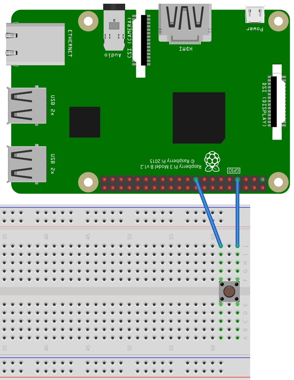
Figure 3.23 – Another circuit for the push button

In the preceding circuit, we connected one end of the push button to pin 7 and the other to a 3V3 pin. Do not connect this end to the 5V pin because when we push the button, it will connect to pin 7 and the GPIO pins can only handle up to 3V3 (3.3 V). Connecting them to a 5V source will damage the pins and the board. Prepare the circuit and make a copy of the code with the following command:

cp prog06.py prog07.py

In the new prog07.py file, we just have to make a small change in the setup() function call, as follows:

GPIO.setup(button, GPIO.IN, GPIO.PUD_DOWN)

This will connect the push button to the internal pull-down resistor. The pin connected to the push button remains set to LOW when the button is open and set to HIGH when the button is pushed. Run the program and the output looks as follows:

Figure 3.24 – The output of the second push button program

The program will show LOW in the beginning. If we push the button, it will become HIGH. The program can be terminated by pressing CTRL + C. This is another way of detecting a key press.

Summary

We learned the basics of Python 3 programming in this chapter. We also learned about the SciPy ecosystem and experimented with the NumPy and Matplotlib libraries. Finally, we saw how to use the GPIO pins of the RPi with LEDs and push buttons.

In the next chapter, we will get started with Python 3 and OpenCV programming. We will also try out a lot of hands-on exercises to learn about programming using a webcam and a RPi camera module.