
Chapter 7: Let's Make Some Noise
In the previous chapter, we learned and demonstrated the concepts of colorspaces and converting them, mathematical transformations, and thresholding operations.
In this chapter, we will learn and demonstrate the concepts related to noise and filtering. This entire chapter is dedicated to understanding the concept of noise in detail. First, we will learn how to simulate various types of noise pattern in depth. Then, we will learn and demonstrate how to use image kernels and the convolution operation. We will also learn how to use the convolution operation to apply various types of filters. Finally, we will learn the basics of low pass filters and demonstrate how to use them to perform blurring and noise removal operations.
We will also use GPIO for demonstrations. In this chapter, we will cover the following topics:
- Noise
- Working with kernels
- 2D convolution with the Signal Processing module in SciPy
- Filtering and blurring with OpenCV
After completing this chapter, you will be able to work with noisy images and reduce the amount of noise in them.
Technical requirements
The code files of this chapter can be found on GitHub at https://github.com/PacktPublishing/raspberry-pi-computer-vision-programming/tree/master/Chapter07/programs.
Check out the following video to see the Code in Action at https://bit.ly/3i7iagG.
Noise
Let's understand the concept of noise in detail. In the field of signal processing, noise is simply just any unwanted signal mixed in with the expected signal. When we talk in terms of noise in images or videos, we can define noise as the undesired variation of intensity and color of pixels. This noise can come from multiple sources.
A few examples include dust on a camera lens, grains in the photo film (this one is desired in analog photography and filmmaking), errors in the CCD sensor and its storage, errors during transmission and reception, and errors while scanning the photograph. A very high amount of noise is not desired. This is because high noise reduces the useful and expected signal, affecting the quality of images.
We can mathematically represent the signal-to-noise ratio with the following formula:
Note:
A higher signal-to-noise ratio means a better quality regarding the signal and the image.
Introducing noise to an image
As discussed in the previous section, there can be multiple sources where noise can originate. We can also introduce noise to a digital image by simulating various types of noise. In this section, we will learn how to simulate salt-and-pepper noise, Gaussian noise, Poisson noise, and random normal noise.
Salt-and-pepper noise
The random introduction of white (salt) and black (pepper) pixels to any image is known as salt-and-pepper noise. We can introduce it to any grayscale image like so:
import numpy as np
import cv2
import random
import matplotlib.pyplot as plt
img = cv2.imread('/home/pi/book/dataset/4.1.03.tiff', 0)
output = np.zeros(img.shape, np.uint8)
p = 0.05
for i in range (img.shape[0]):
for j in range(img.shape[1]):
r = random.random()
if r < p/2:
output[i][j] = 0
elif r < p:
output[i][j] = 255
else:
output[i][j] = img[i][j]
plt.imshow(output, cmap='gray')
plt.title('Salt and Pepper Sprinkled')
plt.axis('off')
plt.show()
In the preceding code, the noise density (denoted by p) is set to 0.05. We are generating a random number for each pixel and if it is less than p/2, we set the pixel to black. If it is between p/2 and p, then we set the pixel to white. Otherwise, the pixel is not modified. Since we are using the random.random() function to generate the noise, the generated noise is different each time we execute the program. The output with the introduced noise looks as follows:
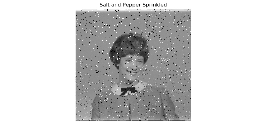
Figure 7.1 – Salt and pepper noise
We can create a small app that adjusts the custom introduced noise with push buttons in the live webcam feed. Now, connect two push buttons to RPi's 7 and 11 GPIO pins in pull-up mode and write the following program:
import RPi.GPIO as GPIO
import cv2
import numpy as np
import random
p = 0.00
cap = cv2.VideoCapture(0)
ret, frame = cap.read()
output = np.zeros(frame.shape, np.uint8)
GPIO.setmode(GPIO.BOARD)
GPIO.setwarnings(False)
button1 = 7
button2 = 11
GPIO.setup(button1, GPIO.IN, GPIO.PUD_UP)
GPIO.setup(button2, GPIO.IN, GPIO.PUD_UP)
In the preceding code, we are initializing the GPIO of the RPi and we are also creating the object for the USB webcam. Now, let's write the logic to adjust the amount of noise we get when pressing the push buttons:
while True:
ret, frame = cap.read()
button1_state = GPIO.input(button1)
if button1_state == GPIO.LOW and p <= 0.1:
p = p + 0.01
if p > 0.1:
p = 0.1
button2_state = GPIO.input(button2)
if button2_state == GPIO.LOW and p > 0:
p = p - 0.01
if p < 0:
p = 0
for i in range (frame.shape[0]):
for j in range(frame.shape[1]):
r = random.random()
if r < p/2:
output[i][j] = 0, 0, 0
elif r < p:
output[i][j] = 255, 255, 255
else:
output[i][j] = frame[i][j]
print(p)
cv2.imshow('Salt and pepper Noise App', output)
if cv2.waitKey(1) == 27:
break
cap.release()
cv2.destroyAllWindows()
The preceding program is computationally expensive because we are computing the noise and the output image continuously. If you are experiencing low frame rates, then reduce the resolution of the USB webcam connected to RPi. The output of the code will be like that shown in the preceding image.
Gaussian noise
This type of noise is named after the mathematician Carl Friedrich Gauss because the values of noise are normally distributed (also known as gaussian distributed). We can simulate this type of noise as follows:
import numpy as np
import cv2
import matplotlib.pyplot as plt
img = cv2.imread('/home/pi/book/dataset/4.1.03.tiff', 0)
row, col = img.shape
img = img.astype(np.float32)
mean = 0
var = 0.1
sigma = var**0.5
gauss = np.random.normal(mean, sigma, (row, col))
gauss = gauss.reshape(row, col)
noisy = img + gauss
print(abs(noisy-img))
plt.imshow(noisy, cmap='gray')
plt.title('Gaussian (Normally distributed) Noise')
plt.axis('off')
plt.show()
The preceding code simulates Gaussian noise of a mean and variance of 0 and 1, respectively, on a grayscale image. We are first converting the image from uint8 into float32 because the noise points can have floating values. We are using the np.random.normal() function to compute the data points for the noise. Note that the amount of noise it produces depends on the values of the mean and variance. For the values we used, the noise is not perceivable to us. Run the code and view the output. It will be as follows:
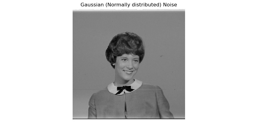
Figure 7.2 – Gaussian (normally distributed) noise
Poisson noise
The noise that is distributed according to the Poisson curve is known as Poisson noise. It is also known as shot noise. This phenomenon occurs because of the particle's nature in terms of light. Let's take a look at some example code where we'll introduce Poisson noise to an image:
import numpy as np
import cv2
import matplotlib.pyplot as plt
img = cv2.imread('/home/pi/book/dataset/4.1.03.tiff', 0)
img = img.astype(np.float32)
vals = len(np.unique(img))
vals = 2 ** np.ceil(np.log2(vals))
noisy = np.random.poisson(img * vals) / float(vals)
print(abs(noisy-img))
plt.imshow(noisy, cmap='gray')
plt.title('Poisson Noise')
plt.axis('off')
plt.show()
The np.random.poisson() function produces random data points distributed along the Poisson curve. These data points are added to the image to create a noisy image with Poisson noise. Run the preceding code and view the output. It will be as follows:

Figure 7.3 – Poisson noise
Random normal noise
We've already seen an example of Gaussian normal noise. We can also generate random normal noise, as follows:
import numpy as np
import cv2
import matplotlib.pyplot as plt
img = cv2.imread('/home/pi/book/dataset/4.1.03.tiff', 0)
img = img.astype(np.float32)
row, col = img.shape
rand_noise = np.random.randn(row, col)
rand_noise = rand_noise.reshape(row, col)
noisy = img + img * rand_noise
print(abs(noisy-img))
plt.imshow(noisy, cmap='gray')
plt.title('Random Normal Noise')
plt.axis('off')
plt.show()
In the preceding code, the NumPy np.random.randn() function creates the data points for the random noise, which are then added to the image. This produces an image with the random noise applied. Run the preceding code and view the output. It will be as follows:
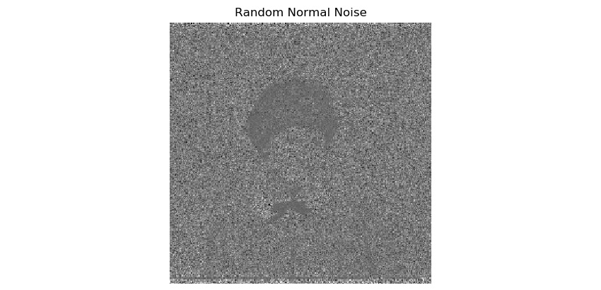
Figure 7.4 – Poisson noise
Working with kernels
Now, let's learn about kernels. We will learn how to use kernels for signal and image processing operations. Kernels are square numerical matrices. Depending on the size and components of the kernel, if we convolve the kernel with the image, we get blurred or sharpened output. Kernels are used for a variety of image processing operations.
Let's look at an example of a simple kernel used for averaging. It can be represented with the following formula:
By using the preceding formula, an averaging kernel that's 3x3 in size can be expressed as follows:

The value of the number of rows and the number of columns is always odd and always the same. They are all square matrices.
We can use the following NumPy code to create the preceding kernel:
K = np.ones((3, 3), np.uint8)/9
Now, we'll learn how to use the preceding kernel and other kernels to process the sample images from the dataset.
2D convolution with the signal processing module in SciPy
Now, let's take a look at the mathematical background of convolution. Convolution is understanding how the shape of a function is affected by another function. The process of computing it and the resultant function is known as a convolution. We can perform convolutions on 1D, 2D, and multidimensional data. Signals are multidimensional entities. Images are a type of signal. So, we can apply convolution to an image.
Note
You can read more about convolution at http://www.songho.ca/dsp/convolution/convolution2d_example.html.
We can perform convolution operations on images with various kernels to process images. For that, we will learn how to use the signal module from SciPy. Let's install the SciPy library with the following command:
pip3 install scipy
We can perform convolution operations on images with various kernels to process images. The function that performs convolution on 2D data is signal.convolve2d(). We must pass a grayscale image and a kernel as arguments to it, which then compute the convolution for the given data. The following is an example:
import scipy.signal
import numpy as np
import matplotlib.pyplot as plt
import cv2
img = cv2.imread('/home/pi/book/dataset/4.1.03.tiff', 0)
k1 = np.ones((7, 7), np.uint8)/49
blurred = scipy.signal.convolve2d(img, k1)
k2 = np.array([[0, -1, 0],
[-1, 25, -1],
[0, -1, 0]], dtype=np.int8)
sharpened = scipy.signal.convolve2d(img, k2)
plt.subplot(131)
plt.imshow(img, cmap='gray')
plt.title('Original Image')
plt.axis('off')
plt.subplot(132)
plt.imshow(blurred, cmap='gray')
plt.title('Blurred Image')
plt.axis('off')
plt.subplot(133)
plt.imshow(sharpened, cmap='gray')
plt.title('Sharpened Image')
plt.axis('off')
The output is as follows:

Figure 7.5 – Performing operations with kernels
As expected, the blur kernel produced a blurred output and the sharpening kernel produced a sharpened image. You may want to change the kernels and observe the effects on the image.
Filtering and blurring with OpenCV
OpenCV also has many filtering and convolution functions. These filtering functions are cv2.filter2D(), cv2.boxFilter(), cv2.blur(), cv2.GaussianBlur(), cv2.medianBlur(), cv2.sepFilter2D(), and cv2.BilateralFilter(). In this section, we will explore all these functions in detail.
2D convolution filtering
The cv2.filter2D() function, just like the scipy.signal.convolve2d() function, convolves a kernel with an image, thus applying a linear filter to the image. The advantage of the cv2.filter2D() function is that we can apply it to data that has more than two dimensions. We can apply this to color images, too.
This function accepts the input image, the depth of the output image (-1 means the input and the output have the same depth), and a kernel for the convolution operation as arguments. The following code demonstrates the usage of this function:
import cv2
import numpy as np
from matplotlib import pyplot as plt
img = cv2.imread('/home/pi/book/dataset/4.2.03.tiff', 1)
input = cv2.cvtColor(img, cv2.COLOR_BGR2RGB)
output = cv2.filter2D(input, -1, np.ones((15, 15), np.uint8)/225)
plt.subplot(121)
plt.imshow(input)
plt.title('Input')
plt.axis('off')
plt.subplot(122)
plt.imshow(output)
plt.title('Output')
plt.axis('off')
plt.show()
The following is the output:
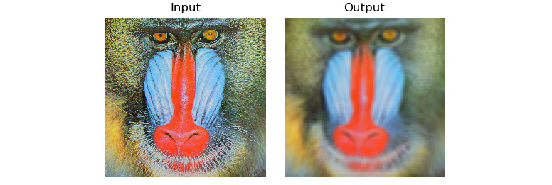
Figure 7.6 – Filtered and blurred versions of the same image
Note:
You can find interactive tutorials on convolution at the following URL: http://micro.magnet.fsu.edu/primer/java/digitalimaging/processing/kernelmaskoperation/
Low-pass filtering
As we discussed earlier, low-pass filters allow low-frequency components to pass through them. Edges and noise are usually high-frequency components. These are filtered out. So, low-pass filters are excellent for noise removal, blurring, and smoothing images.
The OpenCV library offers ready-made functions for performing low-pass filtering. We do not have to write programs from scratch to apply low-pass filters. These functions have code for the kernels written in their definition. We just have to pass arguments to the function and the function automatically creates the kernel and applies it to the image.
The cv2.boxFilter() function accepts the input source image, ddepth, and the size of the kernel as arguments, applies the kernel to the input image, and then returns the blurred image as output. The last parameter is normalize, which could be passed a Boolean value of True or False. This will decide whether the output is normalized. If normalization is passed the True value, the output is multiplied by 1/(number of rows * number of columns), which creates a normalized box filter effect, while if it is passed the False value, the output is multiplied by 1, which creates an unnormalized box filter effect.
The following line shows us an example of a normalized box filter:
output = cv2.boxFilter(input, -1, (3, 3), normalize=True)
The following line shows us an example of an unnormalized box filter:
output = cv2.boxFilter(input, -1, (3, 3), normalize=False)
The cv2.blur() function directly creates a normalized box filter and applies it to the image. We must pass the source input image and the size of the kernel as arguments. We do not have to specify if we want to have normalized output. This will produce the normalized output by default. The following two lines produce the same output:
output = cv2.blur(input, (3, 3))
output = cv2.boxFilter(input, -1, (3, 3), normalize=True)
The OpenCV cv2.GaussianBlur() function applies a Gaussian kernel to the input image. We must pass the input source image and the size of the kernel as arguments to the call of this function. The third parameter is a standard deviation in the direction of the X axis. We are passing 0 as an argument for that. This function filters out all the Gaussian noise in the image. The following is the code example for this:
output = cv2.GaussianBlur(input, (3, 3), 0)
The OpenCV cv2.medianBlur() function applies a median filter and returns a blurred image. This filter is very effective against the images that have the salt-and-pepper type of noise. We need to pass the source input image and a number that defines the size of the square matrix as arguments for the call of this function, as follows:
output = cv2.medianBlur(img, 3)
This function computes the median of all the values of the members of the kernel. The value of the center of the kernel is replaced with the computed value of the median. This is a sliding window type of filter where the window of the matrix of the kernel slides over the matrix of the image and the pixel in the image that overlaps with the center of the kernel matrix is processed with a convolution operation using the computed value of the median.
The cv2.sepFilter2D() function applies a separable linear filter to an image. The following is a sample function call:
output = cv2.sepFilter2D(img, ddepth=-1, kernelX=1, kernelY=1, delta=1)
In the preceding function call, we have the following:
- ddepth: The depth of the output image (-1 if it is the same for the source and target images)
- kernelX: The coefficient for filtering each row
- kernelY: The coefficient for filtering each column
- delta: The constant value that's added to the filtered result
As an exercise for this chapter, you may want to use the cv2.BilateralFilter() function in one of your programs to filter an image.
Summary
In this chapter, we learned about noise and low-pass filtering techniques and how they are used to smooth images. The techniques we learned about in this chapter are very useful if we wish to remove various types of noise from images. You will use these techniques for removing, smoothing, and blurring noise while writing programs for real-life applications such as detecting movement in real time with a USB webcam.
In the next chapter, we will study high-pass filtering techniques and how to detect edges using various functions offered by OpenCV that implement various mathematical morphological operators.