Chapter 8: High-Pass Filters and Feature Detection

In the previous chapter, we learned about kernels and low-pass filters and their applications. We learned about and demonstrated how to use low-pass filters in blurring, smoothing, and de-noising images.

In this chapter, we will learn about and demonstrate the uses of high-pass filters. This includes their application in image processing and computer vision. First, we will explore the Laplacian, Scharr, and Sobel high-pass filters. Then, we will learn about the Canny edge detection algorithm. We will also demonstrate Hough transforms for circles and lines. We will conclude by looking at corner detection with the Harris algorithm.

The following is a list of the topics we will cover in this chapter:

• Exploring high-pass filters
• Working with the Canny edge detector
• Finding circles and lines with Hough transforms
• Harris corner detection

After following this chapter, you will be able to use high-pass filters to detect the features in input images, such as edges, corners, lines, and circles.

Technical requirements

The code files of this chapter can be found on GitHub at https://github.com/PacktPublishing/raspberry-pi-computer-vision-programming/tree/master/Chapter08/programs.

Check out the following video to see the Code in Action at https://bit.ly/2CFnpnD.

Exploring high-pass filters

The concept of high-pass filters is exactly the opposite of low-pass filters. High-pass filters allow high-frequency components of information (such as signals and images) to pass through them. That is why they are known as high-pass filters. In an image, edges are high-frequency components. The kernels we use in high-pass filters boost the intense components in an image. That is why when we apply high-pass filters to images, we get the edges in the output.

Note:

You can read more about high-pass filters at https://diffractionlimited.com/help/maximdl/High-Pass_Filtering.htm. Another type of signal filter is band-pass filters, which allow signals in a range (or band) of frequencies to pass through them. These filters allow us to highlight the edges in images and reduce the noise by using blurring at the same time. You can read more about them at https://homepages.inf.ed.ac.uk/rbf/HIPR2/freqfilt.htm.

OpenCV has a lot of library functions that implement high-pass filters. We will look at how to use the Laplacian(), Sobel(), and Scharr() functions.

Note:

You can learn about the mathematical aspects of high-pass filtering in more detail by referring to the following web pages:

https://www.tutorialspoint.com/dip/Sobel_operator.htm

https://www.tutorialspoint.com/dip/Laplacian_Operator.htm

The following is a list of parameters commonly used by all of the high-pass filtering functions and their meanings:

• src: This is the parameter for the source image in which edges are to be detected.
• ddepth: This is the parameter for deciding the depth of the target image. -1 means the source image and the target image have the same depth. The high-pass filtering functions offered by OpenCV support the following combinations of the depths of source and target images:

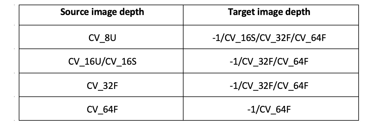
Figure 8.1 – A list of filter functions supported by OpenCV

• dx: This is the order of the derivative of X (this is not required for Laplacian()).
• dy: This is the order of the derivative of Y (this is not required for Laplacian()).
• ksize: This is the size of the matrix for the kernel (this can be 1, 3, 5, or 7 for the Sobel() function or a positive odd number for the Laplacian() function, and it is not required for the Scharr() function).
• scale: This is the scale, which is optional. This is the factor of the optional scale for the computed Laplacian values. Scaling is not applied by default.
• delta: This is the value of delta. This is an optional constant and is added to the final output.
• borderType: This is the method for the extrapolation of pixels for the pixels located at the boundary.

Let's write some code to demonstrate the functionality of the Sobel(), Laplacian(), and Scarr() functions. In the following code, we are computing the Laplacian and the first-order derivative of X of the input image using the Scarr() and Sobel() functions:

import cv2

import matplotlib.pyplot as plt

img = cv2.imread('/home/pi/book/dataset/4.1.05.tiff', 0)

laplacian = cv2.Laplacian(img, ddepth=cv2.CV_32F, ksize=17,

scale=1, delta=0,

borderType=cv2.BORDER_DEFAULT)

sobel = cv2.Sobel(img, ddepth=cv2.CV_32F, dx=1, dy=0,

ksize=11, scale=1, delta=0,

borderType=cv2.BORDER_DEFAULT)

scharr = cv2.Scharr(img, ddepth=cv2.CV_32F, dx=1, dy=0,

scale=1, delta=0,

borderType=cv2.BORDER_DEFAULT)

images=[img, laplacian, sobel, scharr]

titles=['Original', 'Laplacian', 'Sobel', 'Scharr']

for i in range(4):

plt.subplot(2, 2, i+1)s

plt.imshow(images[i], cmap = 'gray')

plt.title(titles[i])

plt.axis('off')

plt.show()

The computation of the derivative of X of the image with the Laplacian(), Scharr(), and Sobel() functions returns the vertical edges in the input image. The following screenshot shows the output of the preceding code:

Figure 8.2 – The x derivative using a high-pass filter

We can connect two push buttons to the 7 and 11 GPIO pins in pull-up configuration and program them to adjust the values of dx and dy. The following is the code to do this:

import RPi.GPIO as GPIO

import cv2

x = 0

y = 1

cap = cv2.VideoCapture(0)

GPIO.setmode(GPIO.BOARD)

GPIO.setwarnings(False)

button1 = 7

button2 = 11

GPIO.setup(button1, GPIO.IN, GPIO.PUD_UP)

GPIO.setup(button2, GPIO.IN, GPIO.PUD_UP)

while True:

print(x, y)

ret, frame = cap.read()

button1_state = GPIO.input(button1)

if button1_state == GPIO.LOW:

x = 0

y = 1

button2_state = GPIO.input(button2)

if button2_state == GPIO.LOW:

x = 1

y = 0

Now, let's compute the output image with the cv2.Scharr() function:

output = cv2.Scharr(frame, ddepth=cv2.CV_32F,

dx=x, dy=y,

scale=1, delta=0,

borderType=cv2.BORDER_DEFAULT)

cv2.imshow('Salt and pepper Noise App', output)

if cv2.waitKey(1) == 27:

break

cap.release()

cv2.destroyAllWindows()

Run the preceding program and observe the edge detection on the live video feed from the USB webcam connected to the Raspberry Pi board. We can also add the X derivative to the Y derivative (computed with Scharr) of the same live video feed, as follows:

import cv2

cap = cv2.VideoCapture(0)

while True:

ret, frame = cap.read()

output1 = cv2.Scharr(frame, ddepth=cv2.CV_32F,

dx=0, dy=1,

scale=1, delta=0,

borderType=cv2.BORDER_DEFAULT)

The previous code segment computes the Scharr derivative of the Y axis. Now, let's write the code for the Scharr derivative of the X axis, as follows:

output2 = cv2.Scharr(frame, ddepth=cv2.CV_32F,

dx=1, dy=0,

scale=1, delta=0,

borderType=cv2.BORDER_DEFAULT)

cv2.imshow('Addition of Vertical and Horizontal',

cv2.add(output1, output2))

if cv2.waitKey(1) == 27:

break

cap.release()

cv2.destroyAllWindows()

Run the preceding program and observe the added X and Y Scharr derivatives. You can implement similar programs with Sobel derivatives. All of these filters are used for detecting edges in the image.

In the next section, we will see how to use high-pass filters to detect edges in an image with the Canny edge detection algorithm.

Working with the Canny edge detector

The Canny edge detection algorithm was developed by John Canny. Canny's algorithm heavily uses the concept of high-pass filters. It has multiple steps.

Note:

You can read more about the Canny edge detection algorithm at http://homepages.inf.ed.ac.uk/rbf/HIPR2/canny.htm.

OpenCV has the cv2.Canny() function, which offers Canny's algorithm. The following are the steps of the algorithm:

1. A Gaussian kernel with a size of 5 x 5 pixels is applied to the input image to remove any noise.
2. Then, we compute the gradient of the intensity of the filtered image. We can use the L1 or the L2 norm for this step.
3. We then apply non-maximum suppression and identify the candidates for the possible sets of edges.
4. The final step is the operation of hysteresis. We finalize the edges depending on the thresholds passed to the images.

   Note:

   You can read more about the L1 and L2 norms and non-maximum suppression at http://www.chioka.in/differences-between-the-l1-norm-and-the-l2-norm-least-absolute-deviations-and-least-squares/ and https://towardsdatascience.com/non-maximum-suppression-nms-93ce178e177c.

The following is a list of parameters for the cv2.Canny() function:

• img: The input source image where we need to detect edges.
• threshold1: The lower bound for the threshold.
• threshold2: The upper bound for the threshold.
• L2gradient: If this value is True, the function uses the L2 norm to compute the set of edges, which is more accurate but computationally expensive. If it is False, then the L1 norm is used to compute the set of edges, which requires less computation but is less accurate.

This function computes and returns the set of detected edges in the source input image. The following code demonstrates this concept well:

import cv2

import matplotlib.pyplot as plt

img = cv2.imread('/home/pi/book/dataset/4.1.05.tiff', 0)

edges1 = cv2.Canny(img, 50, 300, L2gradient=False)

edges2 = cv2.Canny(img, 100, 150, L2gradient=True)

images = [img, edges1, edges2]

titles = ['Original', 'L1 Gradient', 'L2 Gradient']

for i in range(3):

plt.subplot(1, 3, i+1)

plt.imshow(images[i], cmap = 'gray')

plt.title(titles[i])

plt.axis('off')

plt.show()

The output of the preceding code is as follows:

Figure 8.3 – The output of Canny edge detection

We can make the preceding program more interesting by computing the edges in real time, such that the thresholds are adjustable by OpenCV's trackbars:

import cv2

cv2.namedWindow('Canny')

img = cv2.imread('/home/pi/book/dataset/4.1.05.tiff', 0)

def empty(z):

pass

cv2.createTrackbar('Threshold 1', 'Canny', 50, 100, empty)

cv2.createTrackbar('Threshold 2', 'Canny', 150, 300, empty)

while(True):

l1 = cv2.getTrackbarPos('Threshold 1', 'Canny')

l2 = cv2.getTrackbarPos('Threshold 2', 'Canny')

output = cv2.Canny(img, l1, l2, L2gradient=False)

cv2.imshow('Canny', output)

if cv2.waitKey(1) == 27:

break

cv2.destroyAllWindows()

In the previous code, we created two trackbars for the upper and lower thresholds of the Canny algorithm. We used the L1 norm to compute the edges. The output will be as follows:

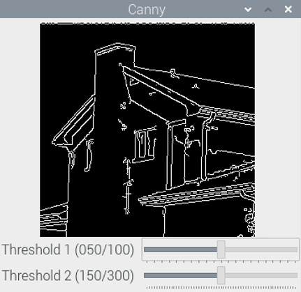
Figure 8.4 – The output of the Canny edge detection algorithm with trackbars

We can apply this algorithm on real-life images, such as a live video feed from our webcam. In the next section, we will learn how to detect circles and lines with the Hough transform.

Finding circles and lines with Hough transforms

OpenCV offers a cv2.HoughCircles() function to detect circles in an image with Hough's method. This returns the centers and radii of the detected circles. It accepts an image, the (cv2.HOUGH_GRADIENT) method of detection, the inverse ratio of the resolution, the minimum distance between the centers of the circles to be detected, the highest threshold of the Canny method used internally, the threshold for the accumulator, and the maximum and minimum distances of the circles to be detected.

Note:

You can find more details about the mathematical aspects of Hough transforms for circles at https://www.cis.rit.edu/class/simg782/lectures/lecture_10/lec782_05_10.pdf.

In the following code, we accept the live video feed from a USB webcam as input. Then, we remove the noise by blurring the input frame, and then we pass the blurred frame to the call of the cv2.HoughCircles() function. Then, we visualize the detected circles with the cv2.Circle() function, as follows:

import cv2

cap = cv2.VideoCapture(0)

while (True):

ret , frame = cap.read()

grey = cv2.cvtColor(frame, cv2.COLOR_BGR2GRAY)

blur = cv2.blur(grey, (5, 5))

circles = cv2.HoughCircles(blur,

method=cv2.HOUGH_GRADIENT,

dp=1, minDist=200,

param1=50, param2=13,

minRadius=30, maxRadius=175)

if circles is not None:

for i in circles [0,:]:

cv2.circle(frame, (i[0], i[1]), i[2], (0, 255, 0), 2)

cv2.circle(frame, (i[0], i[1]), 2, (0, 0, 255), 3)

cv2.imshow('Detected', frame)

if cv2.waitKey(1) == 27:

break

cv2.destroyAllWindows()

cap.release()

Run the preceding program and observe the output. It should look as follows:

Figure 8.5 – The detected circles

The OpenCV cv2.HoughLines() function detects lines in an image. It accepts a grayscale image, the value of rho (the distance accuracy of an accumulator), theta (the angle accuracy of the accumulator), and the parameter of the threshold for the accumulator as arguments. We will demonstrate this with a live USB webcam video feed. The returned output is in polar format, which must be converted into the X/Y coordinate system before visualization:

import numpy as np

import cv2

cap = cv2.VideoCapture(0)

while True:

ret, img = cap.read()

gray = cv2.cvtColor(img, cv2.COLOR_BGR2GRAY)

edges = cv2.Canny(gray, 50, 250, apertureSize=5,

L2gradient=True)

lines = cv2.HoughLines(edges, 1, np.pi/180, 200)

if lines is not None:

for rho,theta in lines[0]:

a = np.cos(theta)

b = np.sin(theta)

x0 = a*rho

y0 = b*rho

pts1 = (int(x0 + 1000*(-b)), int(y0 + 1000*(a)))

pts2 = (int(x0 - 1000*(-b)), int(y0 - 1000*(a)))

cv2.line(img, pts1, pts2, (0, 0, 255), 2)

cv2.imshow('Detected Lines', img)

if cv2.waitKey(1) == 27:

break

cv2.destroyAllWindows()

cap.release()

Run the preceding code and observe its output. The output is as follows:

Figure 8.6 – The detected lines

The Hough transforms must be finely adjusted for the given input. This means that if we cannot see any lines or circles in the correct places, then we can try adjusting the value of the arguments passed to these Hough transform functions. Sometimes, it could produce false results, as in lines and circles will be visible even when there are none in the input frame. Again, for correct results, we must adjust the value of the arguments passed to these functions.

Harris corner detection

OpenCV has the cv2.cornerHarris() function for detecting corners. Its arguments are as follows:

• img: The input image, which must be grayscale and have the float32 type.
• blockSize: This is the size of the neighborhood considered for corner detection.
• ksize: The aperture parameter of the Sobel derivative used.
• k: The free Harris detector parameter used in the equation.

The following is an example program that implements Harris corner detection:

import cv2

import numpy as np

import matplotlib.pyplot as plt

img = cv2.imread('/home/pi/book/dataset/4.1.05.tiff', 0)

img = np.float32(img)

dst = cv2.cornerHarris(img, 2, 3, 0.04)

ret, dst = cv2.threshold(dst, 0.01*dst.max(), 255, 0)

dst = np.uint8(dst)

plt.imshow(dst, cmap='gray')

plt.axis('off')

plt.show()

In the preceding program, we coverted the image into 32-bit float format and then we fed it to the corner detection function. Then, we threshholded the image. We used 0.01*dst.max() as the value of the threshold to compute the binary image. Then, we converted the output into 8-bit integer format so that the output image could be displayed with matplotlib, as follows:

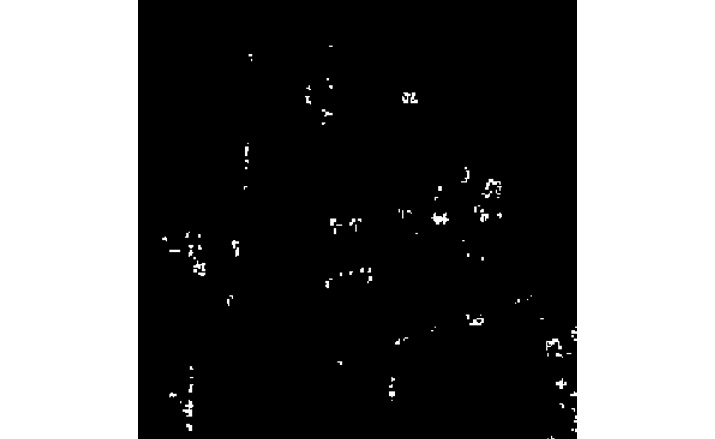
Figure 8.7 – The detected corners

We can use this corner detection method in industrial and robotics applications to detect the corners of regular and predictable objects. It is very useful in real-world automation.

Exercise

To practice what you have learned in this chapter, explore the HoughLinesP(), goodFeaturesToTrack(), and FastFeatureDetector() functions in OpenCV for detecting various features. Write programs using these functions to detect lines using probabilistic Hough transforms and other features.

Summary

In this chapter, we learned the concept and demonstration of high-pass filters. We applied high-pass filters on images to obtain various results. We also demonstrated the various techniques for detecting features, such as corners, lines, edges, and circles. All of these feature-detection algorithms rely on high-pass filtering. Canny's algorithm for edge detection uses Gaussian high-pass filters. The Harris corner detection algorithm uses Sobel spatial derivatives. All of these geometric feature-detection algorithms are routinely employed in real life in industrial automation, smart vehicles, and robotics.

In the next chapter of this book, we will learn the concepts and demonstrate the restoration of degraded images; the segmentation of images; k-means clustering of one-, two-, and multi-dimensional data; image quantization using k-means clustering; and the estimation of a depth map in detail.