Chapter 12: Working with Mahotas and Jupyter

In the previous chapter, we learned about and demonstrated the use of real-life applications in the area of computer vision using Raspberry Pi with OpenCV and Python 3 programming.

In this chapter, we are going to learn the basics of another computer vision library—Mahotas. We are also going to have a look at a Jupyter project and understand how we can use the Jupyter Notebook for Python 3 programming. The topics we will learn in this chapter are as follows:

• Processing images with Mahotas
• Combining Mahotas and OpenCV
• Other popular image processing libraries
• Exploring the Jupyter Notebook for Python 3 programming

After following this chapter, you will be comfortable with using Mahotas for image processing. You will also be able to confidently run Python 3 programs with the Jupyter Notebook.

Technical requirements

The code files of this chapter can be found on GitHub at https://github.com/PacktPublishing/raspberry-pi-computer-vision-programming/tree/master/Chapter12/programs.

Check out the following video to see the Code in Action at https://bit.ly/3fWRYDB.

Processing images with Mahotas

Mahotas is a Python library for image processing and computer vision-related tasks. It was developed by Luis Pedro.

It implements many computer vision-related algorithms. It has been implemented in C++ and it operates on NumPy arrays. It also has a clean interface for Python 3.

Mahotas currently has over 100 functions for image processing and computer vision, and that number keeps growing with every release. This project is under active development and there is a new release every few months. Apart from the added functionality, every new release brings improvements in performance.

Note:

You can learn more about Mahotas by referring to https://mahotas.readthedocs.io/en/latest/.

We can install mahotas on Raspberry Pi with the following command:

pip3 install mahotas

A component of Mahotas will be installed in /home/pi/.local/bin. We can add this to the PATH variable permanently, as follows:

1. Open the ~/.profile file in editing mode by running the following command:

   nano ~/.profile

2. Add the following line to the end:

   PATH='$PATH:/home/pi/.local/bin'

3. Reboot Raspberry Pi:

   sudo reboot

We can verify whether mahotas has been installed successfully by running the following command on Command Prompt:

python3 -c 'import mahotas'

If this command doesn't return an error, then the installation is successful. Now, let's look at creating some programs with Mahotas.

Reading images and built-in images

Mahotas has many built-in images. Let's see how to use them. Look at the following code:

import matplotlib.pyplot as plt

import mahotas

photo = mahotas.demos.load('luispedro')

plt.imshow(photo)

plt.axis('off')

plt.show()

In the preceding code, mahotas.demos.load() is used for loading built-in images to a NumPy array. luispedro is an image of the author of the library. Unlike OpenCV, Mahotas reads and stores color images in RGB format. We can also load and display the image in grayscale mode, as follows:

photo = mahotas.demos.load('luispedro', as_grey=True)

plt.imshow(photo, cmap='gray')

We can load other library images, as follows:

photo = mahotas.demos.load('nuclear')

photo = mahotas.demos.load('lena')

photo = mahotas.demos.load('DepartmentStore')

We can also read the images stored on a disk, as follows:

photo= mahotas.imread('/home/pi/book/dataset/4.1.01.tiff')

This function works in the same way as the cv2.imread() OpenCV function.

Thresholding images

We already know the basics of thresholding. We can threshold a grayscale image by using a couple of functions available in mahotas. Let's demonstrate Otsu's binarization:

import matplotlib.pyplot as plt

import numpy as np

import mahotas

photo = mahotas.demos.load('luispedro', as_grey=True)

photo = photo.astype(np.uint8)

T_otsu = mahotas.otsu(photo)

plt.imshow(photo > T_otsu, cmap='gray')

plt.axis('off')

plt.show()

The mahotas.otsu() function accepts a grayscale image as an argument and returns the value of the threshold. The photo > T_otsu code returns the thresholded image. The following is the output:

Figure 12.1 – Otsu's binarization

We can perform thresholding with the Riddler-Calvard method, too, as follows:

T_rc = mahotas.rc(photo)

plt.imshow(photo > T_rc, cmap='gray')

The mahotas.rc() function accepts a grayscale image as an argument and returns the value of the threshold. The photo > T_rc code returns the thresholded image. Run this and check the output. It will show us a thresholded image with the Riddler-Calvard method.

The distance transform

The distance transform is a morphological operation. It is best visualized with binary (0 and 1) images. It transforms binary images into grayscale images in such a way that the grayscale intensity of a point visualizes its distance from the boundary in the image. The mahotas.distance() function accepts an image and computes the distance transform. Let's look at an example:

import matplotlib.pyplot as plt

import numpy as np

import mahotas

f = np.ones((256, 256), bool)

f[64:191, 64:191] = False

plt.subplot(121)

plt.imshow(f, cmap='gray')

plt.title('Original Image')

dmap = mahotas.distance(f)

plt.subplot(122)

plt.imshow(dmap, cmap='gray')

plt.title('Distance Transform')

plt.show()

This creates a custom image of a square filled with the color black against a white background. Then, it computes the distance transform and visualizes it. This produces the following output:

Figure 12.2 – Distance transform demonstration

Colorspace

We can convert an RGB image into sepia, as follows:

import matplotlib.pyplot as plt

import mahotas

photo = mahotas.demos.load('luispedro')

photo = mahotas.colors.rgb2sepia(photo)

plt.imshow(photo)

plt.axis('off')

plt.show()

The preceding code reads a grayscale image from the library and converts it into an image with sepia colorspace using the call of the rgb2sepia() function. It accepts an image as an argument and returns the converted image. The following is the output of the previous program:

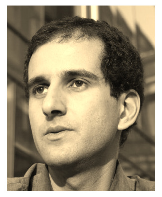
Figure 12.3 – A sepia image

In the next section, we will learn how we can combine the code for Mahotas and OpenCV.

Combining Mahotas and OpenCV

Just like OpenCV, Mahotas uses NumPy arrays to store and process images. We can also combine OpenCV and Mahotas. Let's see an example of this, as follows:

import cv2

import numpy as np

import mahotas as mh

cap = cv2.VideoCapture(0)

while True:

ret, frame = cap.read()

frame = cv2.cvtColor(frame, cv2.COLOR_BGR2GRAY)

T_otsu = mh.otsu(frame)

output = frame > T_otsu

output = output.astype(np.uint8) * 255

cv2.imshow('Output', output)

if cv2.waitKey(1) == 27:

break

cv2.destroyAllWindows()

cap.release()

In the preceding program, we converted a live frame into a grayscale version. Then, we applied a Mahotas implementation of Otsu's binarization, which converted the frame from the live video feed into a Boolean binary image. We need to convert this to the np.uint8 type and multiply it by 255 (all of which takes the form of ones in binary 8-bit) so that we can use it with cv2.imshow(). The output is as follows:

Figure 12.4 – A screenshot of the output window

We usually use the OpenCV functionality to read the live feed from the USB webcam. Then, we can use the functions from Mahotas, or any other image processing library, to process the frame. This way, we can combine the code from two different image processing libraries.

In the next section, we will learn the names and URLs of a few other Python image processing libraries.

Other popular image processing libraries

Python 3 has many third-party libraries. Many of these libraries use NumPy for processing images. Let's have a look at a list of the available libraries:

• skimage (https://scikit-image.org/)
• SimplelTK (http://www.simpleitk.org/)
• scipy.ndimage (https://docs.scipy.org/doc/scipy/reference/ndimage.html)

These are all NumPy-based image processing libraries. The Python imaging library and its well-maintained fork, pillow (https://pillow.readthedocs.io/en/stable/), are non-NumPy-based image manipulation libraries. They also have interfaces to convert images between the NumPy and PIL image formats.

We can combine code that uses various libraries to create various computer vision applications with the desired functionality.

In the next section, we will explore the Jupyter Notebook.

Exploring the Jupyter Notebook for Python 3 programming

The Jupyter Notebook is a web-based interactive interface that works like the interactive mode of Python 3. The Jupyter Notebook has 40 programming languages, including Python 3, R, Scala, and Julia. It provides an interactive environment for programming that can have visualizations, rich text, code, and other components, too.

Jupyter is a fork of the IPython project. All the language-agnostic parts of IPython were moved to Jupyter and the Python-related functionality of Jupyter is provided by an IPython kernel. Let's see how we can install Jupyter on Raspberry Pi:

1. Run the following commands one by one in Command Prompt:

   sudo pip3 uninstall ipykernel

   The previous command uninstalls the earlier version of the ipykernel utility.

2. The following commands install all the required libraries:

   sudo pip3 install ipykernel==4.8.0

   sudo pip3 install jupyter

   sudo pip3 install prompt-toolkit==2.0.5

   These commands will install Jupyter and the required components on Raspberry Pi.

To launch the Jupyter Notebook, log in to Raspberry Pi's graphical environment (directly or using Remote Desktop) and run the following command in lxterminal:

jupyter notebook

This will launch the Jupyter Notebook server process and open a web browser window with a Jupyter Notebook interface, as follows:

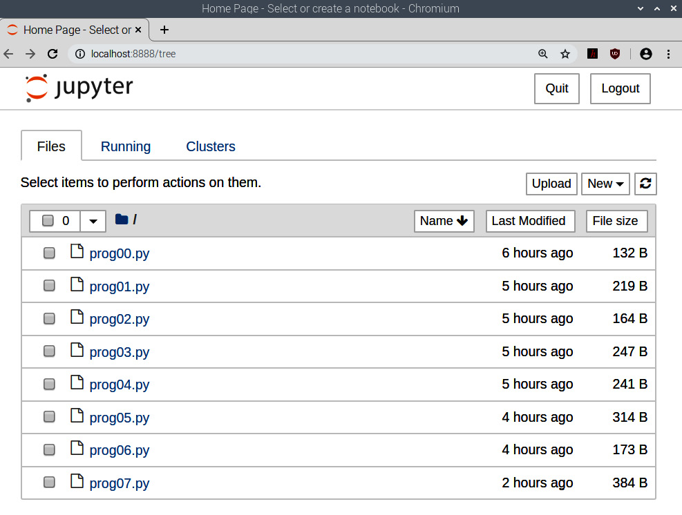
Figure 12.5 – The startup directory

The previous screenshot shows us the directory structure of the directory where we ran the command to launch. I ran it in the directory for the code for our current chapter, /home/pi/book/chapter12. The LXTerminal window where we ran the command shows the server log, as follows:

Figure 12.6 – The Jupyter Notebook server log

Now, let's get back to the browser window that is running Jupyter. In the top-right corner of the browser window, we have options to log out and quit. Below that, we can see the Upload button, the New drop-down menu, and the refresh symbol.

On the right-hand side, we can see three tabs. The first one, as we already saw, shows the directory structure from where we launched Jupyter in Command Prompt. The second tab shows the currently running processes.

Let's explore the New drop-down option on the right-hand side. The following screenshot shows the options available under this menu:

Figure 12.7 – The New menu dropdown

We can see an option for Python 3 under the Notebook section. If you have any other programming languages that use Jupyter, then those languages will also be shown here. We will explore that shortly. The other options are Text File, Folder, and Terminal. The first two options under Other create a blank file and a blank directory, respectively. Terminal, when clicked, launches LXTerminal in a new tab of the browser window, shown in the following screenshot:

Figure 12.8 – Command Prompt running in a web browser tab

If we click on the original tab (listed as Home Page in the browser tabs) and check under the Running option, we can see an entry corresponding to the current terminal window tab, as shown in the following screenshot:

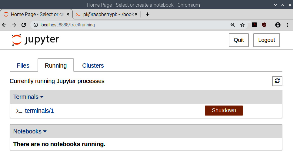
Figure 12.9 – A list of running subprocesses in Jupyter

As we can see, there are options to see the current notebooks and terminals launched under this server. We can shut them down from here. Go to Files and under the New dropdown, select Python 3. This will open a Python 3 notebook under a new tab in the same browser window:

Figure 12.10 – A new Jupyter Notebook tab

We can see that the name of the notebook is Untitled. We can click on the name and it will open a modal dialog box to rename the notebook, as follows:

Figure 12.11 Renaming a notebook

Rename the notebook. After that, in the main Home Page tab, under Files, we can see the test01.ipynb file. Here, ipynb means an IPython notebook. You can see an entry in the Running tab, too. In the /home/pi/book/chapter12/ directory, we can find the test01.ipynb file. Now, let's see how we can use this file for Python 3 programming. Switch to the test01 notebook tab in the browser again. Let's explore the interface in detail:

Figure 12.12 – A Jupyter notebook

We can see a long text area after the In [ ]: text. We can write code snippets here. Make sure that Code is selected from the dropdown of the menu. Then, add the following code to the text area:

print('Hello World')

We can run it by clicking on the Run button in the menu bar. The output will be printed here and a new text area will appear. The cursor will automatically set there:

Figure 12.13 – Running the Hello World! program

The best thing about this notebook is that we can edit and re-execute the earlier cells. Let's try to understand the icons in the menu:

Figure 12.14: The icon buttons in the menu

Let's go from left to right. The first symbol (the floppy disk) is to save. The + symbol adds a text area cell after the currently highlighted cell. Then, we have the cut, copy, and paste options. The up and down arrows are used to shift the current text area cell up and down. Then, we have Run and the interrupt the kernel, restart the kernel, and restart and run the whole notebook buttons. The drop-down box decides the type of the cell. It has the following four options:

Figure 12.15 – Types of cells

If we want the cell to run the code, we choose Code. Markdown is a markup language used for rich text. Select an empty text area cell and change it to the Markdown type. Then, enter # Test into the cell and execute it. This will create a level-one heading, as follows:

Figure 12.16 – A level 1 heading

We can use ## for level-two headings, ### for level-three headings, and so on.

One of the major features of the Jupyter Notebook is that we can even run the OS commands in a notebook. We need to precede the commands with the ! symbol and run them in the cell as Code. Let's look at a demonstration of this. Run the!ls -la command in the notebook and it should produce the following result:

Figure 12.17 – Running OS commands in the Jupyter notebook

We can also show visualizations and images with matplotlib in the notebook. For that, we need to use the magic %matplotlib function. We can use this to set the backend of matplotlib to the inline backend of the Jupyter notebook, as follows:

%matplotlib inline

Let's see a short demonstration of this:

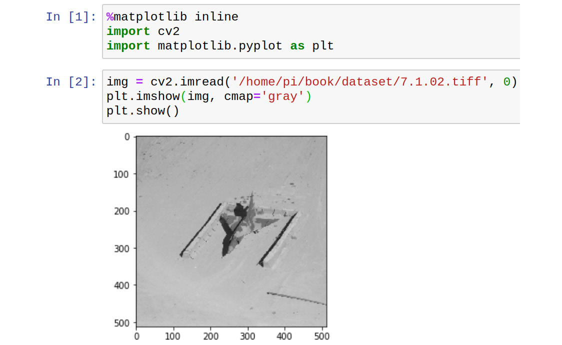
Figure 12.18 – Showing images in the Jupyter notebook

This is how we can show visualizations and images in the notebook itself.

This is a very useful concept. We can have rich text, OS commands, Python code, and output (including visualizations) in a single notebook. We can even share these ipynb notebook files electronically. Just like Python 3, we can use the Jupyter Notebook with a lot of languages, such as Julia, R, and Scala. The only limitation is that we cannot mix code of multiple programming languages in a single notebook.

The last thing I want to explain is how to clear the output. Click on the Cell menu. It looks as follows:

Figure 12.19 – Clearing all the output

We have the Clear option under Current Outputs and All Output. These clear the output of the current cell and the entire notebook, respectively.

I recommend exploring all the options in the menu bar yourself.

Summary

In this chapter, we explored the basics of Mahotas, which is a NumPy-based image processing library. We looked at a few image processing-related functions and learned how to combine Mahotas and OpenCV code for image processing. We also learned the names of other NumPy- and non-NumPy-based image processing libraries. You can explore those libraries further.

The last topic we learned about, the Jupyter Notebook, is very handy for quickly prototyping ideas and sharing code electronically. Many computer vision and data science professionals now use Jupyter notebooks for their Python programming projects.

In the Appendix section of this book, I have explained all the topics that I could not list under this chapter. These topics will be immensely useful to anyone who uses Raspberry Pi for various purposes.