Chapter 1 Real-Time Simulation Using Hybrid Models

The use of computers to simulate the behavior of physical or natural systems is as old as the history of computers itself. Adaptation of physical simulators, such as the original mechanical pilot training simulators, to real-time computer-based simulators was another early development in computer applications. Although the main focus here is on real-time simulation with hybrid models (explained below), the topic of simulation using hybrid models in general will be addressed first, with a more specific treatment of real-time applications introduced later.

The development of a simulation of an actual system involves the creation of a conceptual model of the simuland (the actual system to be simulated), which may be based on a set of rules, or a set of mathematical equations, or some other method of defining the state of the simuland and the way in which it changes with time. We use the term actual system rather than real system because sometimes the simuland does not exist and the use of the term real can be confusing. In the early days of simulation, a distinction quickly arose between two types of model for both real-time and non-real-time simulations. These were referred to as discrete models and continuous models and the associated processes as discrete simulation and continuous simulation. This led to the use of the terms discrete system and continuous system to characterize the actual systems that were being simulated even though it is often not the system that is discrete or continuous but the model that is used to represent it. The practice of referring to the systems themselves as discrete or continuous persists even though many actual systems can be represented by either discrete or continuous models. Traffic flow provides an example. Discrete models are often used in traffic studies in which each vehicle is represented and events such as arrival at an intersection or at a line of stationary traffic or a change of a stop light cause the system state to change. Study of traffic flow on a freeway, where the volume may be much greater is, however, often represented by a continuous model that treats the traffic as if it were a fluid flowing along the freeway using traffic flow rates as model variables.

Discrete and continuous simulations represent two different approaches to the modeling of dynamic systems. Both types of model require the system to be characterized by a system state that changes as time advances. It is the nature of this change that distinguishes the two approaches. A hybrid model is one that includes elements of both discrete and continuous models. Before dealing with hybrid models, we address the relevant features of discrete and continuous models.

1.1.1 Discrete Models

In a discrete model, it is assumed that the system state changes at certain discrete instants of time and remains unchanged between these times. These changes in the state of the system occur instantaneously as the result of an event that triggers them. In a discrete model, time advances from event to event with appropriate updating of the system state at each event time. A prioritized future event queue is usually maintained as a central data structure into which new future events are entered as they are identified, and from which the next event is taken as the simulation clock advances to the next event time.

1.1.2 Continuous Models

In a continuous model, the state of the system is assumed to change in a continuous fashion as defined by the model differential equations, which relate the instantaneous rates of change of system variables to the current state of the system. In practice, the advance of time in the simulation is quasi-continuous because of the discrete time steps adopted by the numerical integration algorithms that are used to generate approximate solutions to the differential equations. In effect, even continuous simulations execute discretely. Switching phenomena are accommodated by allowing local discontinuities to occur in the state variables and their derivatives, in which case the model can be described as piecewise continuous and belongs to a class of hybrid systems discussed below. The details of time management in continuous simulations are also discussed in more detail below.

1.2 Discrete Modeling

As previously stated, a discrete model is one in which the state of the simuland is assumed to change only at specific instances in time. There are two major types of system that can be simulated using discrete models.

1.2.1 Queuing Models

The first and probably most familiar type of discrete model is based on queuing models. In a typical queuing model, entities such as customers or parts arrive at service points representing operators or service units, which process them in turn. The waiting entities form queues, and both the arrival times of new entities and the service times of the servers are often generated from statistical distributions using random number generators. Changes in the state of the system caused by queue arrivals or departures, or a completion of service, are referred to as events and the time at which the event occurs is the event time.

A simulation based on a discrete model establishes an initial state of the system and a future event queue with event timings. The simulation then advances to the first of these event times, and the appropriate changes are made to the system state. These changes may generate changes in the entries in the event queue, including the identification of additional events, and the event queue is modified accordingly. Once the current system state is fully established, the simulation moves on to the next event and the process is repeated. This repeated sequence continues until the simulation satisfies some terminating condition. Models of this kind are used extensively to represent manufacturing plants, distribution networks, service facilities and systems, business operations, and many other applications.

Over time, three main approaches have been developed for simulations that use these models, known as the activity-based, event-based, and process-based methods. Historically, the term activity-based simulation was used to describe simulations in which time advances in small steps with checks for changes at each step. More recently, the term has also been used for Discrete Event System Specification (DEVS) simulations, where only components that are potentially active are evaluated (e.g., in fire spread applications, where only the cells modeling the fire front are evaluated) [1,2]. The original kind of activity-based simulation is inefficient and suitable only for simple applications. Event-based simulation in which time advances from event to event in a single software thread has been the basis of many popular discrete simulation languages, but, as parallel computing options increase, process-based simulation using parallel processors and multiple software threads has become the more popular approach. In this approach, the simulation is divided into processes that can be run in parallel [3]. Each process schedules its events in the correct order, but out-of-order execution can occur in which a process receives an event from another process with an event time that is earlier than its current time. Two strategies are used for dealing with this problem known as conservative and optimistic synchronization. Conservative synchronization requires a process to block its next impending event until it is certain that it is safe. Optimistic synchronization uses a roll-back approach when an out-of-order event occurs. This approach is discussed further in Section 1.2.4.

1.2.2 Digital System Models

As noted above, there are two distinct types of discrete model, the queuing models described in Section 1.2.1 and models that are used to represent systems that can be described by means of difference equations or z-transforms. These digital system models include digital electronic circuits and systems, and sampled-data and digital control systems in which the discrete subsystem is updated at typically equally spaced time intervals [4].

This type of discrete model consists of a set of difference equations that define the next state of the system in terms of its current and past states and its external inputs. If the model is defined, in its entirety or in part, by means of z-transforms, it is usually a straightforward task to convert the z-transform model into difference equation form.

Given a difference equation model, and once the initial state of the system is established, the simulation proceeds by advancing time incrementally by the specified time step and calculating the state of the system at each step. This method is widely used in the simulation of all kinds of digital electronic circuits, computer systems, and digital controllers. As mentioned earlier, a continuous simulation is itself a process of this kind.

1.2.3 DEVS Formalism

In 1976, Zeigler [1] introduced DEVS, a formalism based on General System Theory that provides a means of specifying a mathematical object called a system. The DEVS conceptual framework consists of three basic objects: the model, the simulator, and the experimental frame. The model is a set of instructions that are intended to replicate system behavior, the simulator exercises these instructions to generate the behavior, and the experimental frame describes the way in which the model will be exercised by the simulator. The following description, taken from the introduction to a DEVS tutorial by Zeigler and Sargoujhian [5], draws an interesting comparison between discrete and continuous models:

The Discrete Event System Specification (DEVS) formalism provides a means of specifying a mathematical object called a system. Basically, a system has a time base, inputs, states, and outputs, and functions for determining next states and outputs given current states and inputs. Discrete event systems represent certain constellations of such parameters just as continuous systems do. For example, the inputs in discrete event systems occur at arbitrarily spaced moments, while those in continuous systems are piecewise continuous functions of time.

Although its name, and the above description, suggests that DEVS is restricted to discrete-event models, it has also been extended to continuous models as described by Cellier and Kofman [6]. It is therefore capable of representing hybrid models. Several software products have been developed that are based on DEVS including simulation with continuous and real-time DEVS models [2].

1.2.4 Time Management for Discrete Simulation

The management of time in a discrete simulation is based on knowledge of the times of future events, which are either known a priori or are maintained in a prioritized event queue with priorities that are determined by the time ordering of the events in the queue. It is not necessary to know the time of all events at the start of a simulation but in many cases, as long as the time of the next event is known, time management becomes fairly straightforward. The simulation will begin with a specification of the initial state of the system (length of various queues, status of the queue servers, etc.), and some future events can be determined using the random number generators to generate event times (arrival times, service times, etc.) for the various elements in the system. Time is then advanced to the next event time and appropriate changes made to the state of the system. A queue length may be increased or decreased by an arrival in the queue or by a completion of service; a unit may be seized or released by the simulation and so on. The simulation proceeds alternating between updating the system state as the result of an event and advancing time to the next event. The terminal event time is determined by the termination condition set by the programmer.

As mentioned above, it is becoming common to use a parallel-processing approach to accelerate execution times particularly for process-based discrete simulation software. Using this approach, time may advance in an unsynchronized way on different processors or when using different software threads. This can cause one part of the simulation to advance beyond the generation in another processor or thread of an event that affects it. Conservative scheduling can be used to delay execution of a process until it is safe to do so. Alternatively, optimistic scheduling includes techniques for time to be rolled back so that the effect of an event that has advanced too far in time on the state of the system can be determined. An example of this technique, developed by David Jefferson, is known as Time Warp [7]. Because of the need to facilitate roll back of time, these methods are probably not viable for most real-time applications.

1.2.5 Software for Discrete Simulation

Many software products have been developed over the years aimed at supporting discrete-event simulation. Well-known examples include General Purpose Simulation Systems, Simscript, SIMAN/Arena, Simula, and Dymola/Modelica. The Simula language [8] is notable in that it was the first object-oriented, process-based, discrete simulation language having been first released in the 1960s. As stated above, there are also several software products based on the DEVS formalism.

Simulation of digital electronics, digital control, and sampled-data systems can be accomplished using digital hardware design software such as VHDL or Verilog, which combine a specification of the system with a simulator to test the design.

1.2.6 Example of a Discrete-Event Simulation

A simple example of a discrete-event simulation is described by Matloff and Davis [9]. It involves two machines that break down from time to time and must be repaired. In one variation, a single repair technician is available. Machine uptime and repair time are exponentially distributed with mean values set by the programmer. Events occur when a machine breaks down and when a repair is completed and a machine returns to service. If a second machine breaks down while the first is being repaired, it goes into a waiting queue until the repair technician is available. Clearly, this problem could be extended to include, for example, more machines, possibly with different uptimes and repair times, and different numbers and types of technicians.

1.3 Continuous Modeling

A continuous model is one in which the system state is assumed to vary in a continuous manner with no instantaneous changes in the values of system states or their derivatives.

1.3.1 Nature of Continuous Models

Continuous models normally consist of a mathematical description of the actual system by means of a combination of differential and algebraic equations. This type of mathematical model can be expressed in the form of first-order differential equations, each defining a system state variable, and additional equations that define auxiliary variables. The independent variable is time, producing a mathematical model for a continuously varying dynamic system. Some models may have additional independent variables (usually spatial dimensions), in which case the mathematical model is formulated as a set of partial differential equations. A simple example is the simulation of temperature changes along a thin metal rod as it is heated. The state variable is temperature, and it varies with both time and displacement along the rod. The mathematical model is a partial differential equation with two independent variables, time and displacement.

Simulation using a continuous model involves the initialization of the values of system states followed by calculation of the initial values of the other algebraic variables. This initialization process establishes the initial values of all system variables and is followed by a repetitive process of advancing time in steps using an algorithm for the numerical solution of differential equations. The time steps may be of constant size (usually the case for real-time simulation) or of variable size. Variable-step routines typically include an estimation of the error generated in the current step and a strategy to change the step size to satisfy a user-supplied error tolerance. Such variable-step routines are not normally suitable for real-time simulation because their computation times vary from step to step.

1.3.2 Time Management for Continuous Simulations

Continuous simulations are based on solutions of ordinary or partial differential equations for which time is a continuously changing variable with no instantaneous changes from one value of time to the next, in contrast to the behavior of a discrete simulation in which time jumps from one event time to the next. Computers are programmed to produce approximate solutions of the mathematical model using numerical approximation in which time does advance in small discrete steps. The way in which time advances is specified partly by the programmer and controlled largely by the algorithm chosen by the programmer to solve the equations in the mathematical model. There are many algorithms available for solving differential equations, and the choice of algorithm is one of the key decisions made by the user of a continuous simulation. It will be helpful at this stage to embark on a brief digression about different types and properties of numerical integration algorithms.

1.3.2.1 Types of Numerical Integration Algorithm

Assume a continuous mathematical model of the form

y^{'} \equiv dy / d t = f (y, x, u) (1.1a)

$y^{'} \equiv dy / d t = f (y, x, u) (1.1a)$

x = g (x, y, y^{'}, u) (1.1b)

$x = g (x, y, y^{'}, u) (1.1b)$

where y is a vector of states, y′ is a vector of state derivatives, x is a vector of auxiliary variables (algebraic variables), u is a vector of inputs, and f and g are arbitrary but well-behaved functions.

Numerical integration algorithms normally calculate the next state of a system in terms of the current state and, in some cases, past states. Time is assumed to advance in finite steps leading to equations of the form

y (t + h) = fn (y (t), x (t), u (t)) (1.2)

$y (t + h) = fn (y (t), x (t), u (t)) (1.2)$

where t is current time; h is the time increment for the current step; and y, x, and u are the system state, other system variables, and system inputs, respectively. In many cases, the algorithm can be expanded into a finite or infinite series that matches the Taylor series expansion for the first several terms.

The Taylor series can be expressed as

y (t + h) = y (t) + h y^{'} (t) + (h^{2} / 2!) y^{″} (t) + (h^{3} / 3!) y^{‴} (t) + \dots (1.3)

$y (t + h) = y (t) + h y^{'} (t) + (h^{2} / 2!) y^{″} (t) + (h^{3} / 3!) y^{‴} (t) + \dots (1.3)$

The simple Euler integration method, for example, solves Equations 1.1a and 1.1b by calculating

y (t + h) = y (t) + h y^{'} (t) (1.4)

$y (t + h) = y (t) + h y^{'} (t) (1.4)$

In other words, Euler integration simply extrapolates the states, y, by assuming that the derivatives of y remain constant throughout the step and equal to the value at the start of the step. The process is illustrated in Figure 1.1.

Assume a first-order system,

y^{'} (t) = f (y, t) (1.5)

$y^{'} (t) = f (y, t) (1.5)$

Images

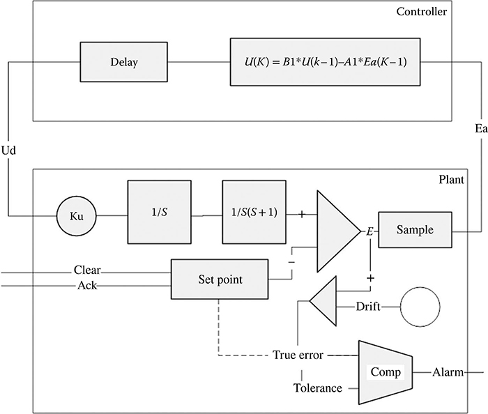
FIGURE 1.1 Euler integration.

Figure 1.1 shows part of the true solution for a state variable, y(t). The initial value of y is y₀ at time t = t(0). The initial value of the derivative, from Equation 1.5, is given by

y^{'} (t_{0}) = f (y_{0}, t_{0}) (1.6)

$y^{'} (t_{0}) = f (y_{0}, t_{0}) (1.6)$

Applying Euler integration over a step of length h, we have

y (t_{0} + h) = y (t_{0}) + h y^{'} (t_{0}) (1.7)

$y (t_{0} + h) = y (t_{0}) + h y^{'} (t_{0}) (1.7)$

The derivatives at (t₀ + h) can now be calculated from

y^{'} (t_{0} + h) = f (y_{0} + h, t_{0} + h) (1.8)

$y^{'} (t_{0} + h) = f (y_{0} + h, t_{0} + h) (1.8)$

This process can be repeated until the final time is reached.

This algorithm matches the first two terms in the Taylor series (up to the term in the first derivative, y′) and is known as a first-order method. More complex methods are available that match the Taylor series to the terms in y″ (second-order methods), y‴ (third-order methods), and so on. These Taylor-series-based methods attempt to approximate the solution over a single step using a polynomial approximation, linear for first order (Euler), a quadratic for second-order methods, and so on. An alternative approach, based on exponential approximations, will be introduced in Section 1.5.3. In general, a method of order n will have an approximation error dependent on the neglected terms of the Taylor series, which are the terms in hⁿ⁺¹ and above. This error is known as the truncation error. Additional errors can arise from the accumulation of round-off error, particularly when using lower-precision data formats and large numbers of steps. As we shall see, this can be of particular importance in some real-time simulations. There are many different numerical integration algorithms available. Runge–Kutta methods of different orders are widely used. Fourth-order Runge–Kutta methods are often chosen as providing a good trade-off between accuracy and computational complexity [10].

The two major factors that affect the accuracy of a numerical integration are order and step size. Generally speaking, errors decrease with decreasing step size and increasing order. In extreme cases, steps can be so short that round-off error can become an issue, particularly with lower-precision data formats. As step size increases, some algorithms can become unstable, even when the unstable behavior appears at a point at which errors were, up to that point, acceptable. In other words, acceptable stable solutions can make a rapid transition to unacceptable unstable solutions with very small increases in step size.

1.3.2.2 Fixed versus Variable Step

One of the choices faced by users of continuous simulation is whether to use an algorithm that advances time in equal increments (a fixed-step algorithm) or one that varies the size of time increments in order to satisfy user-supplied error tolerances. Modern variable-step routines often use an approach in which estimated solutions of order n and n − 1 are generated at each step, and the error estimate is based on the difference between the two. The justification for this is that this difference approximates the value of the last term in the Taylor series before truncation. This is assumed to be a conservative estimate of the total truncation error. The default routine in MATLAB^® and Simulink^® [11] (ODE45) is, for example, a method of this type that compares fifth- and fourth-order approximations to the solution.

Fixed-step routines are simpler and are favored for real-time simulation because they result in a constant computation time. Variable-step routines are safer, popular, and often used as defaults in those simulation systems that offer a choice of algorithms.

1.3.2.3 Explicit versus Implicit

Algorithms that calculate the next state in terms of the current (and possibly earlier) states have right-hand sides that can be evaluated directly and are referred to as explicit algorithms. For some algorithms, however, Equation 1.2 is modified to include one or more terms in (t + h) on the right-hand side:

y (t + h) = fn {y (t), y (t + h), x (t), x (t + h), u (t), u (t + h)} (1.9)

$y (t + h) = fn {y (t), y (t + h), x (t), x (t + h), u (t), u (t + h)} (1.9)$

which results in an implicit formula. This normally necessitates the solution of a set of simultaneous algebraic equations in each step. If the system of equations is linear, this can often be done by direct calculation, but nonlinear systems require an iterative solution procedure at each step. Implicit methods are generally unsuitable for real-time simulation because the amount of computation can vary from step to step without an a priori known upper bound. Moreover, it may prove necessary to provide external hardware-in-the-loop inputs ahead of time (i.e., u(t + h) may be required at time t). Implicit methods can, however, offer improved stability and are often used for stiff systems (see Section 1.3.2.5).

1.3.2.4 Single-Step versus Multistep

The methods discussed so far are self-contained within each step and are called single-step methods. Some methods spread the calculation over more than one step and are called multistep methods. For example, the value of the system state at the next step may be determined in terms of the system state at the current and previous step times. Some algorithms require data from the past three or four steps. Equation 1.2 is now modified as follows:

y (t + h) = fn {y (t - k), x (t - h), u (t - h)}, where k = 0, 1, 2, \dots (1.10)

$y (t + h) = fn {y (t - k), x (t - h), u (t - h)}, where k = 0, 1, 2, \dots (1.10)$

These methods are often cost-effective (in terms of the amount of computation necessary to achieve a given accuracy), but they do require special procedures to start them since past data is not available at the start of the simulation. These methods can also cause problems with hybrid and real-time simulations.

1.3.2.5 Variable-Order Algorithms and Stiff Systems

Many integration algorithms experience stability problems when applied to stiff systems. Stiff systems are systems that have a wide variation in the system dynamics, often described as having widely varying time constants or eigenvalues. These systems are characterized by containing both high-speed and low-speed dynamic properties, all of which must be captured by the method of solution. When the high-speed modes are active (i.e., variables are changing rapidly), short step sizes, commensurate with the time constants involved, are necessary to capture the rapid changes of state. The major problem with stiff systems arises when the fast modes are inactive (i.e., damped out) and the solution trajectories are smooth. Typically, longer steps would be used to cover the smooth trajectories, but in a stiff-system simulation, the dormant high-frequency modes can be stimulated by the integration algorithm causing instability unless the step size remains short, which can be very time-consuming.

This problem is often addressed by the use of special stable, stiff-system algorithms. One of the best known is the method of Gear [12], an implicit method based on backward differentiation, which adjusts the order as well as the step size of the algorithm to maintain both accuracy and stability while minimizing the amount of computation required. The original Gear DIFSUB routine was subsequently improved by Hindmarsh in the widely used GEAR routine [13]. Variable-order, variable-step methods of this kind are not normally suitable for time-critical real-time simulations.

1.3.2.6 Difference Equations

Whichever method is chosen to solve the differential equations in the mathematical model, the effect is to convert them into a set of approximately equivalent difference equations. It is these difference equations that are actually evaluated in each step of the simulation, and the way in which this process is implemented can have a significant bearing on the way the simulation is coded, particularly for real-time applications.

1.3.3 Software for Continuous Simulation

There is a long history of languages for continuous simulation (traditionally referred to as continuous system simulation languages or CSSLs) dating back to the 1950s and 60s. Initially the software available to support continuous simulation developed from analog computer techniques. Analog computers used specially designed electronic amplifiers that were configured to perform mathematical operations such as integration, addition, multiplication, and function generation. These amplifiers were connected together by the programmer using patch cords to represent the differential equations to be solved. System constants and parameters were set on potentiometers (variable voltage dividers). The first continuous simulation systems for digital computers mimicked this approach. Names such as DAS (Digital Analog Simulator) and MIDAS (Modified Integration DAS) [14,15] were common. These systems required the programmer to produce a flow diagram showing the interconnection of components (adders, multipliers, integrators, etc.), which were similar to the physical components of an analog computer. In effect, the digital program simulated an analog computer simulation of the system! Since graphical input was not available, the flow diagrams were entered in tabular form showing how the various inputs and outputs were interconnected (similar to the Netlist for a modern electric circuit simulator such as SPICE). The expressiveness of this approach was limited by the available repertoire of components, and flow diagrams based only on these primitive elements rapidly became very large. With the increasing popularity of general-purpose high-level programming languages such as FORTRAN and Algol 60, a demand developed for simulation languages in which the program could be expressed in terms of program statements rather than flow diagrams. To distinguish between the two approaches, the names block-structured (for the flow-diagram method) and statement-structured (for the statement-based languages) were introduced. The emergence of statement-structured simulation languages as a replacement for the block-structured simulators was hailed as a great step forward.

The statement-structured languages include CSMP (Continuous System Modeling Program), DSL (Digital Simulation Language), ACSL (Advanced Continuous Simulation Language), CSSL4 (Continuous System Simulation Language 4), ESL (European Simulation Language), and, more recently, MATLAB and Simulink. An important development was the publication, in 1967, of a specification for a CSSL by Simulation Councils, Inc. (SCi) in their journal SIMULATION [16]. Although this specification was far from providing a complete standard, it did provide a template for the CSSLs that followed its publication. One of its main and enduring features was a simulation execution structure made up of three main regions designated the Initial, Dynamic, and Terminal regions. These names are fairly self-explanatory with calculations at time zero (or some other user-specified initial time) performed in the Initial region, the solution of the mathematical model with advancing time in the Dynamic region, and the terminating conditions and postrun calculations in the Terminal region.

Later, by virtue of the combination of greatly increased computer power and inexpensive graphical displays, a new generation of block-structured simulation software was developed. Modern continuous simulation software typically provides a graphical editor by means of which a flow diagram of the system can be defined. Unlike the original block-structured languages, modern simulation software offers a hierarchical approach in which primitive elements can be combined into more complex components and added to libraries. Extensive libraries are available from the software vendors, and users also have the capability of developing their own model libraries. Some products still provide the user with access to an underlying equivalent statement-structured form of the program, which experienced users can revise to meet special needs. Current versions of ESL and ACSL, for example, provide this feature.

With modern graphically based simulation languages, the user is able to build a block diagram of the simuland, often using simulation elements selected from toolboxes of common components and subsystems. The management of the simulation is implicit and controlled by the user through the use of interactive screens by which the parameters of the simulation (e.g., start time, terminating condition, integration algorithm and step size, output details, etc.) are selected. Some critics view the use of toolboxes with concern, claiming that this removes the details of the precise nature of the models used from the user and that this has the potential to generate convincing but inaccurate simulations. Used with care, however, and with adequate knowledge of the details of the model of each subsystem, this approach provides a very convenient way to develop simulations quickly.

1.3.4 Example of a Continuous Simulation

Consider the simple example of a small metal sphere that has been heated to a temperature T₀ at time t = 0 and is cooling down in air with an ambient temperature T_a. The differential equation that describes this process, at least approximately, is

d T / d t = K (T_{a} - T) given T (t = 0) = T_{a} is the ambient temperature (1.11)

$d T / d t = K (T_{a} - T) given T (t = 0) = T_{a} is the ambient temperature (1.11)$

Note that we can calculate the initial value of dT/dt = K*(T_a − T₀). If T_a < T₀, then dT/dt will be negative, indicating cooling, and if T_a > T₀, then dT/dt is positive for heating. Using the Euler method, this would produce an estimate for T(h) of

T (h) = T_{0} + h * K * (T_{a} - T_{0}) (1.12)

$T (h) = T_{0} + h * K * (T_{a} - T_{0}) (1.12)$

The derivative dT/dt at T = h can then be calculated and the process repeated until the terminating condition is reached.

The process is the same for more complex integration algorithms or for larger systems of differential equations. In all cases, the calculation alternates between the determination of the current values of derivatives and auxiliary variables and the use of the integration algorithm to advance time by one step and calculate the corresponding values of the state variables. This alternation between establishing the current system state and advancing time mirrors the process used in discrete simulations in which the advance of time to the next event time alternates with the reevaluation of the system state.

1.4 Hybrid Models

In simple terms, a hybrid model is one that contains characteristics of both discrete and continuous models. There is extensive literature on the theory and analysis of hybrid systems (e.g., Ref. [17]).

For the purposes of developing simulations, a hybrid system can be viewed in some cases as a basically discrete model containing one or more states that change in a continuous fashion between events, and in others as a basically continuous model in which the states change continuously for most of the time but in which one or more of the states or their derivatives can occasionally change instantaneously. In yet other cases, the discrete and continuous processes may be balanced in an integrated model that is equally distributed between discrete and continuous components.

This distinction is important. Many currently available simulation software products provide comprehensive support for either discrete or continuous models with limited additional features that support the alternate approach. The balance between discrete and continuous elements in the model will, therefore, often dictate the choice of software to perform the simulation.

1.4.1 Time Management for Hybrid Simulations

Regardless of the balance between discrete and continuous elements in a model, time management for hybrid simulations requires synchronization between the processing of events and the continuous advance of time for the continuous elements. In some cases, a period of continuous simulation, which may be of limited duration, can be triggered by a discrete event. In this case, time-management control will switch from the discrete to continuous modes with the duration of time steps determined by the integration algorithm. The simulation will remain in continuous mode until either the continuous simulation terminates (generating another event) or an event occurs in the discrete part of the model that impacts the continuous part. It can cause the continuous simulation to terminate, or it can cause a change of input or even a change to the continuous mathematical model in some way. Conversely, changes in the state of the continuous system can generate new discrete events, for example, when a continuous variable exceeds some critical value, such as a temperature or pressure limit.

When discrete events are occurring during a period in which a continuous process is active, it is important to manage the time advance of the continuous process so that the end of a step coincides with the time of an event. In this regard, it is helpful to use a distinction, first introduced by Cellier [18], between time events and state events.

A timed event is one for which the event time is known in advance. An example would be a clock signal in a sampled-data system. The numerical integration step size should, where possible, be controlled so as to coincide with the known timing of timed events.

A state event is one that is triggered by a condition that depends on the values of state or other dynamic variables in the simulation, such as a temperature that rises above a set point. The nature of state events is such that their event times are not normally known in advance, and special procedures are required to process them.

In non-real-time applications, synchronization with both types of event is often achieved by using a variable-step integration algorithm and additional synchronization procedures between the discrete and continuous simulations. In real-time applications, it may be necessary to reduce the step size of a fixed-step integration algorithm to minimize timing errors. In the case of state events, the discrete event is triggered by the continuous simulation, and it is again necessary either to use a variable-step algorithm to ensure accurate timing of the event or, particularly for real-time applications, to adopt a sufficiently short step size.

1.4.2 Software for Hybrid Simulations

Several software packages that were originally developed specifically for either discrete or continuous simulation have subsequently added features that support hybrid simulations.

Early work on developing numerical integration routines to handle discontinuities was carried out by Hay, Crosbie, and Chaplin [19,20]. They adapted a conventional fourth/fifth-order variable-step routine by adding an interpolation stage that is activated whenever an end-of-step check shows that a state event occurred during the step. They used a succession of interpolations, starting with a linear interpolation between the start and end of the step to produce a first approximation to the event time. This is followed by a quadratic interpolation using values at the start, approximate event time, and end of step to produce a more accurate value for the event time. Further iterations with third- and higher-order interpolations are possible but not normally necessary to locate the event time with acceptable accuracy. This approach is very effective in non-real-time simulation and has been widely adopted, but it is not suitable for real-time simulation because of the variable and extended computation time whenever a state event occurs within a step.

This technique was later included in ESL, one of the first continuous simulation languages to introduce methods for processing discontinuities accurately and automatically. ESL was developed for the European Space Agency by Hay, Crosbie, and Pearce [21]. The way in which the discontinuities (events) are specified by the user is elegant and is based on the use of logical statements and a program construct known as a when clause. A when clause is a section of code that is executed when and only when (i.e., once only) a specified condition becomes true. More conventional conditional if statements can also be used to switch between different descriptions of a subsystem. Almost any discontinuous element can be described using if and when constructs.

A simple example of the use of the when clause is the code for a submodel for a T flip-flop. This device is assumed to toggle its single logical output whenever a trigger is applied to its input, which can be specified in ESL as

SUBMODEL TFLOP(LOGICAL:flag:=LOGICAL:trigger);
                INITIAL
                  flag:=false;
                DYNAMIC
                  when trigger then
                    flag:=not flag;
                  end_when;
              END TFLOP;

The first line defines a submodel named TFLOP that has a single logical output named flag and a single logical input named trigger. The flag is set to false in the INITIAL region. In the DYNAMIC region, which is executed at each time step, the flag is inverted when and only when the logical variable trigger changes from false to true. More statements could be inserted between when and end_when, and all of them would be executed whenever the trigger becomes true.

A more complex example, using both if and when, is illustrated by the following code template, which implements a method of defining a system that switches between three different states. A line preceded by a double hyphen (--) is a comment line.

INITIAL
-- Initialize state
   state := 1; DYNAMIC
   when state=1 AND transition12 then
      state := 2;
   when state=1 AND transition13 then
      state := 3;
   when state=2 AND transition21 then
      state := 1;
   when state=2 AND transition23 then
      state := 3;
   when state=3 AND transition31 then
      state := 1;
   when state=3 AND transition32 then
      state := 2;
   end_when
-- Assign variables depending on state
   v1 :=if state=1 then <expression11>
         else_if state=2 then <expression12>
         else_if state=3 then <expression13>;
--Repeat for all variables

It is assumed that the simulation is initialized with the system in State 1. There may be additional initialization code in the INITIAL region. The DYNAMIC region uses when clauses to define the six possible transitions between the three states by means of the logical variables transition12, etc, which are normally all false. A state transition is indicated by setting the corresponding transition variable to true. The values of variables in a particular state are set using conditional if statements. Note that these are structured as assignments (:=) with conditional right-hand sides.

One of the strengths of ESL is that once a discontinuity has been defined in the code using if or when constructs (or by selecting a graphical element that is itself defined using such statements), it is automatically recognized and implicitly detected when the software runs with appropriate control of the step size. When models containing such discontinuities are simulated using a variable-step integration routine, and when the value of one of the transition variables changes from false to true, a discontinuity detection mechanism is invoked that adjusts step sizes in a way that ensures that the event time coincides with the end of an integration step, within a user-specified tolerance. This approach is not ideal for real-time simulation unless it can be guaranteed that the process will always reach a satisfactory conclusion within the available frame time. ESL does, however, support real-time simulation of these hybrid systems. The object-oriented modeling language Modelica [22] and the MathWorks product Simscape^™ [23] also use the notion of if and when statements and corresponding semantics. Other languages, including ACSL and Simulink, have provided alternate ways of defining state events based on the definition of crossing detectors. Additional coding is usually necessary to link the specification of the event to its processing during execution.

Turning now to models that are basically discrete, some older discrete languages have added features for handling continuous elements. Simscript, for instance, features a continuous process that is illustrated by an example in the next section.

As stated earlier, when it was first developed in 1976, the DEVS formalism and the software products that implemented it were focused on discrete models. In the 1990s, continuous features were developed. We have already established that a numerical solution of differential equations is, in effect, a discrete process and is therefore accessible to representation using the DEVS formalism. It is necessary to capture the difference equations that arise from the continuous mathematical model combined with the selected numerical integration algorithm with DEVS. With a feature of this kind, a DEVS implementation is clearly capable of handling hybrid models. One example is PowerDEVS [24], a version of DEVS aimed specifically at power-electronic circuits and systems, but capable of supporting a range of hybrid simulations including real-time simulations. PowerDEVS is also interesting in that it uses a QSS (Quantized State System) [6,25] approach to continuous simulation. QSS deals with systems in which system states, as well as time, change in finite increments. Simulations using QSS thus involve discretization of both time and state variables.

1.4.3 Examples of Hybrid Simulations

Understanding hybrid simulation techniques can be made easier by initially separating them into three groups: those that are basically continuous with discrete elements, those that are basically discrete with continuous elements, and those that are equally balanced. These distinctions can best be illustrated by simple examples.

1.4.3.1 Continuous Model with a Discrete Element

One of the most commonly quoted examples of a hybrid system in the literature is the bouncing ball. A bouncing ball simulation provides an example of a continuous model (dynamics of the motion of the ball) with discrete elements (impact with a hard surface). In its simplest form, the continuous model equates the acceleration of the ball to acceleration due to gravity (d²x/dt² = −g for x > 0) and assumes a hard impact in which the velocity of the ball changes instantaneously (dx/dt⁺ = −k*dx/dt), where the coefficient of restitution k is a dissipation factor.

Another simple example, which will be developed later, is provided by the electrical circuit in Figure 1.2. An alternating current supply feeds a load consisting of a resistor and capacitor in parallel through a series resistance and a diode. The diode is represented by a very simple model of an ideal switch. If the voltage across it is positive, its resistance is assumed to be zero and the diode can be represented by a short circuit. If the voltage is negative, the resistance is infinite and the diode is represented by an open circuit. The voltage produced by the supply is v = Vcos(wt). Assuming the capacitor is initially discharged, the initial value of v is equal to V and the diode will conduct. A simple mathematical model can be produced that recognizes two modes of operation of the circuit, the conducting mode and the nonconducting mode.

1.4.3.1.1 Conducting Mode

Assuming ideal components, the key differential equation is provided by the relationship between voltage and current for the capacitor, which can be expressed as

i_{c} = C d v_{c} / d t or d v_{c} / d t = i_{c} / C (1.13)

$i_{c} = C d v_{c} / d t or d v_{c} / d t = i_{c} / C (1.13)$

where

i_c = i – i_R

i_c = (v – v_c)/R_L

i_R = v_c/R_L

Images

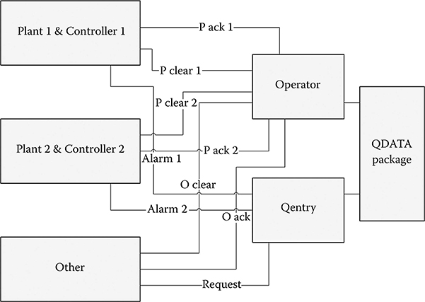
FIGURE 1.2 Example of a hybrid model: An electric circuit containing a switch.

The sequence of calculation is as follows:

The value of the state v_c is known at the beginning of a time step, either as an initial condition or the result of the calculation from the previous step. Given the value of v_c at the current time t, it is possible to calculate the values of i_R, i, and i_c also at time t (in addition to v, which is defined for all time in the model). Given i_c, it is then possible to calculate the current value of the derivative dv_c/dt. This completes the computation of the state of the system at the given time instant. This is the point at which the algorithm chosen by the user to solve the differential equation takes over. Time is advanced by one time step, and the value of v_c at time t + h, where h is the time increment, is calculated using the integration algorithm. A simple example would be to use Euler integration, which simply assumes that the value of dv_c/dt at t is maintained constant over the next time increment so that the new value of v_c is calculated as

v_{c} (t + h) = v_{c} (t) + h v_{c}^{'} (t), where v_{c}^{'} = d v_{c} / d t (1.14)

$v_{c} (t + h) = v_{c} (t) + h v_{c}^{'} (t), where v_{c}^{'} = d v_{c} / d t (1.14)$

The process is then repeated starting at t = t + h with the corresponding value of v_c and is continued until the system mode changes to nonconducting or the terminating condition for the simulation is reached.

1.4.3.1.2 Nonconducting Mode

In the nonconducting mode, the RC load is disconnected from the supply. The governing equations are now

d v_{c} / d t = i_{c} / C (1.15)

$d v_{c} / d t = i_{c} / C (1.15)$

where

i_c = – i_R

i_R = v_c/R_L

Given v_c at the beginning of a time step, i_R and i_c can be calculated followed by dv_c/dt. The numerical integration algorithm can then be used to calculate v_c at the end of the next step.

A key question now is how to make the decision to switch between modes. As was discussed earlier, the answer to this question can be quite different for real-time and non-real-time simulations. When real-time execution is not required, a variable-step algorithm, preferably one that is combined with a discontinuity detection scheme, could be most appropriate. For real time, it may be necessary to use a fixed-step method, in which case the length of the step is constrained by the need to limit timing errors. This question is discussed further in Section 1.5.1.

1.4.3.2 Example of a Discrete-Based Hybrid Simulation

Discrete models are widely used to represent industrial processes. Many of these models deal with the progress of materials or components as they move through a manufacturing process. Objects are held in queues waiting for equipment to become available to perform the next stage in the manufacturing process. Service times are often generated randomly using an appropriate distribution. In some cases, it is necessary to represent the process more accurately, and this may involve the use of a continuous model of a particular part of the total manufacturing process. Fayek [26] describes an application involving the movement of metal ingots into and out of a furnace.

A steel plant has a soaking pit furnace which is being used to heat up steel ingots. The interarrival time of the ingots is determined to be exponentially distributed with a mean of 1.5 hours. If there is an available soaking pit when an ingot arrives, it is immediately put into the furnace. Otherwise it is put into a warming pit where it is assumed to retain its initial temperature until a soaking pit is available.

Fayek describes both totally discrete and combined continuous–discrete (or hybrid) models to address this problem. In the discrete version, the time to heat an ingot in the furnace is uniformly distributed between 4 and 8 hours. In the hybrid version, it is determined by solving a differential equation representing the change in temperature of the ingot:

d h / d t = (H - h_{i}) * c_{i} (1.15)

$d h / d t = (H - h_{i}) * c_{i} (1.15)$

where h_i is the 1000°F temperature of the ith ingot, H is the furnace temperature (assumed to be 1500°F), and c_i is the heating time coefficient of the ith ingot, which is equal to (0.07 + x), where x is normally distributed with a mean of 0.05 and a standard deviation of 0.01.

Ingots are to be heated to a final temperature that is normally distributed between 800 and 1000°F.

In a further variation of the simulation, the furnace temperature is assumed variable. It is normally heating up toward a given final temperature and is also reduced when cold ingots are put into the furnace. This adds a second differential equation for the furnace temperature as follows:

d H / d t = (2500 - H) * 0.05 (1.16)

$d H / d t = (2500 - H) * 0.05 (1.16)$

Introducing a cold ingot is assumed to produce an instantaneous fall in the furnace temperature depending on the difference between the furnace and ingot temperatures divided by the number of ingots in the furnace. This hybrid simulation was implemented in a version of Simscript V that supports continuous features. The simulation ran successfully, and the ability to model the dynamics of the heating and cooling effects provided a more valid representation of the entire process.

1.4.3.3 Balanced Hybrid Simulation

Many of the documented applications involving hybrid simulations are of the above kinds, either mainly discrete or mainly continuous. An example of a more balanced hybrid simulation is provided by a study performed for the European Space Agency by the author and colleagues using ESL [27]. It involves an artificially created simulation that was intended to demonstrate the ability of ESL to perform simulations that combined a balance of continuous and queuing elements. This is not generally a straightforward task with most simulation software systems. It contains continuous and both types of discrete elements discussed earlier (queues and sampled data).

The continuous model (derived from an ACSL example) is illustrated in Figure 1.3. It contains a subsystem with a transfer function 1/s(s + 1). The output, X, of this system is compared to a set point X_c to form an error signal E. A sampled version of E is passed to a digital controller, which generates a control signal U. The control is a linear combination of the current error, E(n), the previous error, E(n − 1), and the previous control, U(n − 1). The difference equation describing the controller is

U (n) = B 1 * U (n - 1) + A 0 * E (n) - A 1 * E (n - 1) (1.17)

$U (n) = B 1 * U (n - 1) + A 0 * E (n) - A 1 * E (n - 1) (1.17)$

The constants A0, A1, and B1 depend upon the equivalent lead and lag time constants of the controller (T_lead and T_lag) and the sampling period T_s. A delay is added to the updating of U to represent the computation delay in the digital controller.

This basic example was extended (see Figure 1.4) by making the assumption that the actual set point, unknown to the controller, is drifting (represented by an additional sinusoidal variation). It is assumed that a mechanism exists for indicating when the true error from the actual set point exceeds a given threshold by generating a logical alarm signal. This alarm message is transmitted over a communication link to an operator console where it is queued with other messages until the operator is available to take corrective action. A correction message is then sent back to the system, which has the effect of resetting the set point. The system also has the ability to determine when the alarm condition clears spontaneously, in which case it sends a cancellation message, which will cancel the original alarm if it is received before the alarm has been acted upon. This system incorporates the following features of combined continuous/discrete systems:

State events generated from within a continuous subsystem
Synchronous A/D sampling of continuous variables
Updating of continuous variables through a D/A converter
Components described by difference equations/z-transforms
Digital computation delays
Queuing of events awaiting processing
Cancellation of queued events
A server (operator) responding to queued events in sequence

Images

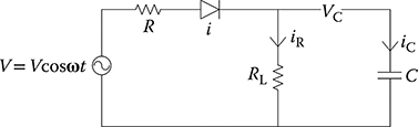
FIGURE 1.3 Continuous part of combined continuous–discrete benchmark.

Images

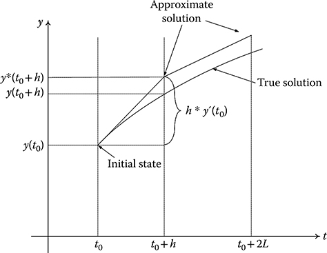
FIGURE 1.4 Combined continuous–discrete benchmark.

The entire simulation was coded in ESL using ESL primitives. ESL is a traditional CSSL with discrete features. It is to be expected that more recent hybrid simulation software products that are aimed specifically at hybrid systems would facilitate the development of simulations of this kind.

One of the outcomes of this study was a list of recommended enhancements to the ESL language to make it more capable of supporting balanced hybrid models with features similar to those in the benchmark. These included

Add support for discrete variable types and a notation for difference equations
Support the use of z-transforms
Improve processing of time events
Introduce an EVENT block for defining state and time events
Support queues so that they can be easily specified and manipulated by the user
Provide a greater range of random number distributions
Provide support for user-specified statistical outputs
Provide support for producing results in the form of event lists

These changes were aimed at producing a more balanced hybrid simulation capability. Most of them remain unimplemented.

1.5 Real-Time Hybrid Simulation

Most real-time simulations are characterized by the necessity to incorporate some physical component in the simulation. This can be hardware, software, or a human or humans in the loop. In all cases, it is necessary for the simulation to be synchronous with a real-time clock to ensure correct timing of the interactions between the simulation and the external agent.

1.5.1 Timing Issues in Real-Time Hybrid Simulation

Challenges face the potential user of hybrid simulation, whether real time or not. The choice of software to support the development of the simulation can be critical, and using it to properly represent both the continuous and discrete features of the model and their interaction requires great care. Precise time management, particularly the accurate interchange of timing control between discrete and continuous processes, is essential. At this point, it is necessary to draw a distinction between integration step size and frame time in real-time simulations. The integration step size is precisely what it says, the increment of time by which the current time is advanced in a single application of the selected numerical integration algorithm. In real-time simulation, it is normally constant. The frame time is the normally constant time interval between data transfers to external elements such as hardware in the loop or other simulations, and a frame may consist of several integration time steps. It can be regarded as a real-time equivalent of the communication interval in standard CSSL terminology. The required frame time can dictate the choice of integration algorithm, especially for higher-speed, real-time simulations with the need for very short frame times.

Taken together, these factors pose a formidable challenge to the designer of hybrid real-time simulations. We now consider some of the specific issues that arise in their creation.

The basic requirement for a real-time simulation is that all computation within a frame should be completed within the fixed frame time. In some applications, this requirement can be relaxed, allowing occasional data drops (perhaps caused by communication delays, for example, with hardware-in-the-loop), but in general, the hard real-time requirement must be observed.

The detailed nature of real-time hybrid simulations depends to some extent on the length of the acceptable frame time, which can vary, in different types of applications, from seconds to microseconds. For longer frame times, the ability of the processor or processors to perform the necessary calculations in the available time is less often an issue, but time synchronization between different parts of the simulation, particularly in those cases where the simulation is distributed over different systems, is key.

Distributed real-time simulations often involve different software components to be integrated into a joint simulation. The question of interoperability between software elements then becomes of major concern. Special software environments have been developed to support this kind of interoperability. One of the most widely used is the high-level architecture (HLA) [28]. This architecture is widely used, particularly in military applications, where different simulations running on different platforms in different geographical locations are involved. An HLA simulation is known as a federation and its components as federates. Data that is passed between different federates using a publish-and-subscribe technique is time stamped to ensure that time synchronization is maintained using a real-time interface.

Wainer, Kim, et al. [29,30] have described some interesting DEVS-based real-time hybrid simulations, which make use of an interface that supports combinations of model components that use different DEVS-based software. A simulation of a robot that negotiates obstacles uses PowerDEVS to simulate the robot and ECD⁺⁺ (another DEVS-based software) to simulate the interaction with the obstacles.

A number of commercial systems are available that support real-time hybrid simulations including MathWorks xPC Target^™ [31] and Real-Time Windows Target^™ [32], the combination of National Instruments (NI) LabView with MathWorks Simulink using the Simulation Interface Toolkit from NI [33], RT-Lab from OPAL-RT [34], the rtX simulator from Applied Dynamics International [35], and the Real-Time Digital Simulator (RTDS), a simulator that specifically targets electrical power systems, from RTDS Technologies [36].

1.5.2 High-Speed Real-Time Hybrid Simulation

Particular problems arise with those applications that involve short intervals between repeated discrete events. This is true for instance of real-time simulations of modern power-electronic systems. Electric power can be delivered in many different forms. The most obvious distinction is between alternating current (ac) and direct current (dc). Although line frequencies of 50 or 60 Hz are commonly used for domestic supply, other frequencies may be used. For example, 400 Hz is a common choice for many power distribution systems, in aircraft for example. Higher frequencies require smaller transformers, filters, and other related equipment but involve higher losses over longer distances. Many pieces of equipment (such as computers, phones, radios, televisions, for example) require dc supplies and commonly incorporate a converter from ac to dc in the line cord. The dc voltages vary for different applications and for both ac and dc supplies, there are different limits on the amount of allowable harmonic distortion (unwanted ac frequencies).

Converters convert electric power both ways between ac and dc. Converters involve a significant amount of switching whether they are producing dc from an ac waveform or vice versa. The switching is often controlled by pulse-width modulation controllers that vary the intervals between switching events while keeping the average frequency constant. In modern converters, the switching frequencies are set as high as possible to minimize harmonic distortion and to limit the size of associated components. For higher power applications (such as the power system for an electric ship), switching frequencies may be in the kilohertz range. For small appliances, frequencies may be measured in tens or even hundreds of kilohertz. For a 10 kHz switching frequency, the average interval between switching events is 100 μs. In a non-real-time simulation, a variable-step integration algorithm with discontinuity detection would probably be used to minimize errors in the timing of the switching event. In a real-time simulation, using a fixed-step integration algorithm, timing errors are minimized by using sufficiently short steps. If, for example, the maximum allowable timing error is 2% of the average period of the controller switching waveform, then the step size should be no longer than 2 μs. The worst case arises when the actual switch time is immediately after the end of a step. In this case, the integration step will proceed using the equations that were valid before the switching event for the entire step, and the corresponding simulated switching event will not occur until the end of the step. In this case, the timing error is equal to the integration step length. Techniques aimed at compensating for switch-timing errors in real-time simulations are discussed in Section 1.5.3.

Note that real-time simulations that require frame times of less than about 10–20 μs require special processing systems because conventional real-time simulation systems are not capable of reliably maintaining such short frames. Digital signal processors (DSPs) [37] and field-programmable gate arrays (FPGAs) [38] have been used for this purpose. The DSPs or FPGAs need not be more powerful (in a MFLOPS sense) than the conventional system. The key is that the processor that executes the critical simulation code is not vulnerable to interruption by the operating system. A dedicated core or cores in a multicore processor could also be employed in this manner. The RTDS power-system simulator uses both DSPs and FPGA-based processors and offers high-speed units capable of 2-μs frame times.

1.5.3 Numerical Integration for High-Speed Real-Time Simulation

Methods to address the need for short frame times in high-speed real-time (HSRT) simulation can be divided into the use of simple algorithms that minimize the amount of computation and the use of techniques that compensate for midstep switching events.

As discussed earlier, the simplest integration algorithm is provided by the Euler method, which only requires that the derivatives of system variables at the start of a step (all of which are known) are multiplied by the fixed-step length to provide an estimate of the change in the value of each variable during the step. This simple extrapolation has the advantage of simplicity. It is not widely used in general in continuous simulations because of its larger truncation errors, but in cases where the step size is constrained for other reasons, it can be effective. It does, however, present stability concerns. Euler integration is the simplest of a class of single-step methods of different orders, known as Runge–Kutta methods, which produce an approximation to the average rate of change of a state variable during a step. Stability margins for integration algorithms can generally be expressed in terms of the eigenvalues of the system (which can be viewed as corresponding roughly to inverse time constants). Euler integration becomes unstable if the step size exceeds twice the shortest time constant (more strictly 2/λ, where λ is the largest eigenvalue). This situation can arise at a point at which slightly shorter (stable) step lengths produce acceptably accurate results, so the transition from acceptable to totally unusable results can be immediate. For nonlinear systems with eigenvalues that can change from step to step, this can be a serious problem. It is consequently advisable for users to be fully aware of the dynamics of their systems and of the potential for numerical instability. Higher-order Runge–Kutta methods have slightly improved stability behavior, but the margin is still, in general, no more than about 2.8/λ (an improvement of only about 40% over the Euler method). One of the advantages of using variable-step algorithms is that they usually ensure that the step length remains in the stable region, but their use is not normally an option in real-time simulation.

Another option for real-time simulation is a fixed-length, explicit, multistep method such as Adams–Bashforth. This approach has been advocated by Robert M. Howe [39], who has a long history of innovative contributions to real-time simulation methodology. Howe has also developed techniques specifically for switched linear circuits, such as those found in power-electronic applications, that compensate for the fact that switching instants occur during a step [40]. Howe’s approach involves splitting a step into substeps separated by switching events and calculating analytic solutions to the differential equations using precomputed coefficients. These techniques require additional computation but can also reduce errors significantly. They permit the use of longer steps for the same accuracy at a cost of more computation per step, and they represent a serious option for HSRT simulation involving linear differential equation models.

De Kelper et al. [41] has also developed techniques for minimizing the effect of switching errors in real-time simulations of electrical power systems that adapt the methods for non-real-time variable-step integration described in Section 1.4.2 to fixed-step methods, particularly for real-time applications. De Kelper has adapted the method to real-time fixed-step simulations in two ways. The first is to limit the interpolation to a single linear process, and the second is to advance the solution from the switching point by the same fixed-step length but to again use linear interpolation to produce a solution at the end of the original step. In other words, the first step goes from t to t + h and is interpolated to find a solution at t + d, which is the time at which the linear interpolation locates the switching event. The second step goes from t + d to t + d + h, and a linear interpolation is used to produce a solution at t + h.

Bednar and Crosbie [42] has developed an efficient integration method for linear models that builds on a state-transition approach [43]. The state-transition approach is based on the solution to the vector differential equation

d x / d t = A x + B u (1.18)

$d x / d t = A x + B u (1.18)$

Assuming a sample and hold input,

u (t) = u (k T) for k T < = t < (k + 1) T (1.19)

$u (t) = u (k T) for k T < = t < (k + 1) T (1.19)$

then the approximate solution is

x [(k + 1) T] = Φ * x (k T) + Γ * u (k T) for k = 0, 1, \dots (1.20)

$x [(k + 1) T] = Φ * x (k T) + Γ * u (k T) for k = 0, 1, \dots (1.20)$

where Φ is the transition matrix.

This approach provides a class of fixed-step, explicit methods of varying complexity and accuracy depending on how many terms of two infinite series are used. A version using three and two terms, respectively, and known as the ST(3,2) method has proved effective. In a number of tests, it compared favorably with other methods for accuracy, stability, and computation time. The method can also be applied to some nonlinear systems of equations [44].

1.5.4 HSRT Multirate Simulation

Most applications that require HSRT simulation involve components with lower bandwidth dynamics that do not require the short frame-time that HSRT methods are designed to deliver. In these cases, it is better to design a multirate simulation in which the system is separated into segments that are simulated using different frame rates. This means that those segments that do not depend on HSRT techniques can be implemented on conventional processors. A multirate benchmark has been devised to support the study of high-speed, real-time, multirate simulations.

Multirate simulation has been a recognized simulation technique for many years (e.g., Ref. [45]). It has often been used to accelerate the execution of large simulations. The basic idea is that it is not necessary to update the dynamics of the slower parts of a system at the same rates as are required for the faster parts. It is a simple idea that has stood the test of time when applied carefully and conservatively. It is particularly suitable for HSRT applications for which it is possible to execute the high-speed segments on the special high-speed processors and the slower segments on more conventional computer systems.

It is not, however, without its problems. Step sizes for the different segments must be chosen with care. It is also necessary to distinguish between integration step size and communication interval. The segments in a multirate simulation communicate with each other at communication intervals that are normally related by integer multiples. Within a communication interval, the simulation can proceed using a single integration step, equal in length to the communication interval, or by using several integration steps, which together advance the simulation by the duration of one communication interval. These integration steps can be of either fixed or variable length as long as synchronism with the communication interval is maintained.

A multirate simulation is effectively a sampled-data system, and issues can arise with the adequacy of the data passed between segments, particularly when a faster segment has to wait several communication intervals before it receives an update from a slower segment. The input from the slow segment can be kept constant between updates (zero-order hold), but this introduces an effective time delay of approximately half the slower frame time. Extrapolation techniques (first-, second-, or even fractional-order hold) can be used to compensate. Another question is how data is passed from a faster to a slower segment given that the faster segment will produce several data points between data transfers to the slower one. Some method of averaging the fast outputs over each slow frame is required. There is a danger of aliasing if rapidly changing outputs from a fast segment are not filtered or averaged in some way. In some cases, this can be achieved by carefully selecting the segment boundaries so that the outputs from the fast segment do not have high-frequency components. In other cases, it may be necessary to add antialiasing filters. If sufficient care is not taken in selecting communication intervals and data interchange processes, multirate simulations can become inaccurate or even unstable.

A multirate benchmark simulation, based on a simulation of an unmanned underwater vehicle (UUV), was developed in cooperation with the University of South Carolina and the University of Glasgow [46,47]. The UUV uses a battery bank as its energy source feeding an ac motor drive through a dc to ac converter. The drive powers the vessel, which is modeled as a six-degree-of-freedom platform with control surfaces. The system is divided into subsystems that are simulated with different frame rates: (1) converter and switching controller (fast), (2) feedback controller (slow medium), (3) motor drive (fast medium), and (4) the vessel, battery, and interface graphics (slow). The UUV system is illustrated in Figure 1.5. Typical simulation frame rates used in this simulation are

Battery, ship, 3D graphics: 100 mS
Converter, switch controller: 2–5 μS
Motor: 50–100 μS
Feedback controller: 1 mS

Images

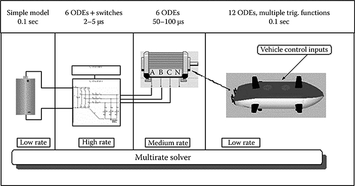
FIGURE 1.5 Simplified representation of unmanned underwater vehicle model (vessel inputs and outputs and controls are omitted).

The simulation has been implemented using the Virtual Test Bed (VTB), developed by the University of South Carolina [48] in both non-real-time and real-time versions. As an indication of the increase in speed afforded by the use of multirate techniques, implementations of this simulation on a Microsoft Windows system running in non–real time showed a speedup of three orders of magnitude from versions that used the fastest rate for the entire system, with no significant change in the accuracy of the results. The VTB provides a flexible simulation environment with 2D and 3D graphics for output and user controls. It supports multidisciplinary simulation with both mechanical and electrical components and has a library containing a large range of electrical and mechanical components.

The real-time version replaced the UUV drive system (motor and propulsion drive shaft) with hardware. It was not feasible to reproduce the actual physical components in the laboratory, so a small low-power motor was used to represent the actual motor. The load on the drive shaft was represented by a generator coupled to the motor output shaft. The output of the generator was connected to a programmable resistive load that was controlled by the simulation. This configuration supported an equivalent real-time simulation of the UUV system that could support the development of high-speed, real-time, multirate simulation techniques.

1.6 Concluding Remarks

In this chapter, we have considered relevant aspects of discrete and continuous as well as hybrid simulations in both real-time and non-real-time contexts. The main focus, however, is on real-time simulation with hybrid models. We have seen that the distinction between discrete and continuous simulation is, in a sense, a distinction without a difference since a continuous simulation is itself essentially a discrete process. The key to hybrid simulations lies in the approach to time management and the synchronization of events between different parts of the simulation.

First we consider the non-real-time requirements. In general, discrete simulations usually advance in unequal time steps from event to event, and continuous simulations are also more likely to advance in unequal time steps using variable-step algorithms. Both discrete and continuous simulations can use fixed time steps. They are commonly used for simulating discrete time systems such as digital controllers and are a feature of the older activity-based discrete simulation approach. Where possible, however, the use of variable time steps can deliver significant improvements in performance.

For real-time simulation, the important factor is the available computer speed. If the computer is capable of executing code significantly faster than the related real events, then it can be allowed to idle while real events catch up. In fact, although it is often stated that variable-step integration algorithms are unsuitable for real-time continuous simulations, their use, particularly in conjunction with a fixed frame time, is not unfeasible as long as the longest possible execution time for the calculations within a frame can be guaranteed to be less than the time available.

For real-time hybrid simulations, time management must be capable of advancing the continuous simulations in fixed time steps (or frames) toward the time of the next discrete event. Synchronizing the fixed increment of time applied to the continuous simulation with the variable increments between events in the discrete simulation is a key factor in the time-management protocol. In the UUV simulation described above, the continuous simulation time steps are sufficiently short so that the timing errors that result from imposing a fixed time step are assumed to be acceptable. The methods described by Howe [39,40] and De Kelper et al. [41] help to compensate for these errors. An alternative, more widely used for non-real-time simulations, would be to use the methods that locate the time at which imminent state events occur and adjust the step size to coincide with the event. In real time, however, this introduces a double step in which time first advances to the time of the state event and then continues to the end of a normal step. This can only be done if the available processor power can accommodate the double step plus the overhead associated with locating the state event. The situation can be further complicated by multirate techniques, which require the event handler to keep track of the different sequences of fixed increment events for the different rates as well as the discrete events for each multirate segment.

Developing real-time hybrid simulations is in many cases a challenging undertaking with today’s available simulation software products. The picture is most promising for applications that are dominantly discrete with limited continuous elements or dominantly continuous with discrete elements restricted to switching events. Adding a need for more complete and balanced discrete/continuous features similar to the example described above, or for high-speed, or for multirate simulation significantly increases the degree of difficulty and is very likely to involve detailed programming of algorithms and time management. With the increasing interest in all kinds of hybrid simulations, there are growing and exciting opportunities for simulation software developers to meet this need.

References

1. Zeigler, B. P. 1976. Theory of Modeling and Simulation. 1st ed. New York: Wiley Interscience.

2. Wainer, G. A., and P. J. Mosterman, eds. 2011. Discrete-Event Modeling and Simulation: Theory and Applications. Boca Raton, FL: CRC Press.

3. Fujimoto, R. M. 2003. “Advanced tutorials: Parallel Simulation: Distributed Simulation Systems.” In Proceedings of the 2003 Winter Simulation Conference, edited by S. Chick, P. J. Sánchez, D. Ferrin, and D. J. Morrice, New Orleans, LA, December 7–10, 2003, pp. 124–134.

4. Olukotun, K., M. Heinrich, and D. Ofelt. 1998. “Digital System Simulation: Methodologies and Examples.” In Proceedings of 35th Design Automation Conference, DAC ’98, San Francisco, CA, June 15–19, 2011, pp. 658–663.

5. Zeigler, B. P., and H. S. Sarghoujian. 2003. “Introduction to DEVS Modeling & Simulation with JAVA: Developing Component-based Simulation Models.” http://www.acims.arizona.edu/PUBLICATIONS/publications.shtml#devsHLA.

6. Cellier, F. E., and E. Kofman. 2006. Continuous System Simulation. New York: Springer Verlag.

7. Jefferson, D. et al. 1987. “The Time-Warp Operating System.” In Proceedings of 11th Symposium on Operating Systems Principles. New York: ACM.

8. Birtwistle, G. M., O.-J. Dahl, B. Myhrhaug, and K. Nygaard. 1973. SIMULA Begin. Chartwell-Bratt, Bromley, England 1979.

9. Matloff, N. “Introduction to Discrete-Event Simulation and the SimPy Language,” http://heather.cs.ucdavis.edu/~matloff/156/PLN/DESimIntro.pdf.

10. Ralston, A., and P. Rabinowitz. 2001. A First Course in Numerical Analysis. 2nd ed. Mineola, NY: Dover Publications.

11. Klee, H., and R. Allen. 2011. Simulation of Dynamic Systems with MATLAB and Simulink. Boca Raton, FL: CRC Press Inc.

12. Gear, C. W. 1962. Numerical Initial Value Problems in the Numerical Solution of ODEs. New York: Wiley.

13. Byrne, G. D., A. C. Hindmarsh, K. R. Jackson, and H. G. Brown. 1977. “A Comparison of Two ODE Codes: GEAR and EPISODE.” Computers & Chemical Engineering 1 (2): 133–147.

14. Clancy J. J., and M. S. Fineberg. 1965. “Digital Simulation Languages: A Critique and a Guide.” In Proceedings of the November 30–December 1, 1965, Fall Joint Computer Conference, 23–26. Montvale, NJ: AFIPS Press.

15. Brennan R. D., and R. N Linebarger. 1964. “A Survey of Digital Simulation: Digital Analog Simulator Programs.” SIMULATION 3 (6): 22–36.

16. SCi Software Committee. 1967. “The SCi Continuous System Simulation Language (CSSL).” SIMULATION 9 (6): 281–303.

17. Goebel, R., R. G. Sanfelice, and A. R. Teel. 2009. “Hybrid Dynamical Systems.” IEEE Control Systems Magazine 29 (2): 28–93.

18. Cellier, F. E. 1979. Combined Continuous/Discrete System Simulation by use of Digital Computers, Doctoral dissertation, ETH Zurich.

19. Hay, J. L., R. E. Crosbie, and R. I. Chaplin. 1974. “Integration Subroutines for Systems with Discontinuities.” Computer Journal 17 (3).

20. Crosbie, R. E., and J. L. Hay. 1974. “Digital Techniques for the Simulation of Discontinuities.” In Proceedings of Summer Simulation Conference, Houston, TX, July 9–11, 1974, pp. 87–91.

21. Crosbie, R. E., S. Javey, J. L. Hay, and J. G. Pearce. 1985. “ESL—A New Continuous System Simulation Language.” SIMULATION 44 (5): 242–246.

22. Modelica Association. March 2010. “Modelica: A Unified Object-Oriented Language for Physical Systems Modeling: Language Specification, Version 3.2.” https://www.modelica.org/documents/ModelicaSpec32.pdf.

23. MathWorks. September 2009. Simscape User’s Guide. Natick, MA: MathWorks.

24. Bergero, F., and E. Kofman. 2010. “PowerDEVS: A Tool for Hybrid System Modeling and Real-Time Simulation.” SIMULATION 87 (1–2): 113–132.

25. Kofman, E., F. E. Cellier, and G. Migoni. “Continuous System Simulation and Control.” In Discrete-Event Modeling and Simulation: Theory and Applications, edited by G. A. Wainer and P. J. Mosterman, 75–107. Boca Raton, FL: CRC Press.

26. Fayek, A-M. 1987. Introduction to Combined Discrete-Continuous Simulation Using PC SIMSCRIPT II.5. La Jolla, CA: CACI.

27. Crosbie, R.E. August 1993. “Combined Continuous-Discrete Simulation.” ISIM Internal Report ref estecextlab sk4_fin.001, ISIM International Simulation Ltd, 161 Claremont Rd. Salford M6 8PA, UK.

28. Kuhl, F., R. Weatherly, and J. Dahmann. 1999. Creating Computer Simulation Systems: An Introduction to the High-Level Architecture. Upper Saddle River, NJ: Prentice Hall PTR.

29. Moallemi, M., and G. Wainer. 2010. “Designing an Interface for Real-Time and Embedded DEVS.” In Proceedings of Symposium on Theory of Modeling and Simulation (DEVS10), Orlando, FL, April 11–15, 2010, SCS.

30. Cho, S. M., and T. G. Kim. 1998. “Real-Time DEVS Simulation: Concurrent, Time-Selective Execution of Combined RT-DEVS Model and Interactive Environment.” In Proceedings of 1998 Summer Computer Simulation Conference, Reno, NV, July 19–22, 1998, SCS.

31. Ledin, J., M. Dickens, and J. Sharp. 2003. “Single Modeling Environment for Constructing High-Fidelity Plant and Controller Models.” In Proceedings of 2003 AIAA Modeling and Simulation Technologies Conference, Austin, TX, August 21–24, 2003.

32. MathWorks. Real-Time Windows Target^™. Natick, MA: MathWorks. http://www.mathworks.com/products/rtwt/

33. Isen, F. W. 2009. DSP for MATLAB and LabVIEW: Synthesis Lectures on Signal Processing. San Rafael, CA: Morgan and Claypool.

34. Venne, P., J-N. Paquin, and J. Belanger. “The What, Where and Why of Real-Time Simulation.” http://www.opal-rt.com/technical-document/what-where-and-why-real-time-simulation.

35. Applied Dynamics International. http://www.adi.com/products_sim_tar_rtx.htm.

36. Forsyth, P., and R. Kuffel. 2007. “Utility Applications of a RTDS Simulator.” In Proceedings of Power Engineering Conference (IPEC 2007), 112–17, December 3–6. Piscataway, NJ: IEEE Press.

37. Crosbie, R. E., J. J. Zenor, D. Word, and N. G. Hingorani. October–December 2004. “Fast Real-Time DSP Simulations for On-Line Testing of Hardware and Software.” Modeling & Simulation 3 (4).

38. Word, D., J. J. Zenor, and R. Powelson. 2008. “Using FPGAs for Ultra-High-Speed Real-Time Simulation.” In Proceedings of Conference on Grand Challenges in Modeling and Simulation, Edinburgh, Scotland, June 16–19, 2008.

39. Howe, R. M. 1985. “Transfer Function and Characteristic Root Errors for Fixed-Step Integration Algorithms.” Transactions of the Society for Computer Simulation, 2 (4): 293–300.

40. Howe, R. M. 2010. “Improving Accuracy and Speed in Real-Time Simulation of Electric Circuits.” International Journal of Modeling, Simulation, and Scientific Computing 1 (1): 47–83.

41. De Kelper, B., L. A. Dessaint, K. Al-Haddad, and H. Nakra. 2002. “A Comprehensive Approach to Fixed-Step Simulation of Switched Circuits.” IEEE Transactions on Power Electronics 17 (2): 216–224.

42. Bednar, R., and R. E. Crosbie. 2007. “Stability of Multi-Rate Simulation Algorithms.” In Proceedings of the Summer Computer Simulation Multiconference, San Diego, CA, July 16–19, 2007, SCS San Diego.

43. Ogata, K., 1987. Discrete-Time Control Systems, State Space Analysis. Englewood Cliffs, NJ: Prentice Hall.

44. Bednar, R., and R. E. Crosbie. 2009. “Solution of Non-Linear Differential Equations Using State-Transition Methods.” In Proceedings of Conference on Grand Challenges in Modeling and Simulation, Istanbul, Turkey, July 13–16, 2009, SCS.

45. Palusinski, O. A. 1985. “Simulation of Dynamic Systems Using Multi-Rate Integration Techniques.” Transactions of SCS 2 (4): 257–273.

46. Zenor, J. J., R. Bednar, and S. Bhalerao. 2008. “Multi-Party, Multi-Rate Simulation of an Unmanned Underwater Vehicle.” In Proceedings of Conference on Grand Challenges in Modeling and Simulation, Edinburgh, Scotland, June 16–19, 2008.

47. Zenor J. J., D. J. Murray-Smith, E. W. McGookin, and R. E. Crosbie. 2009. “Development of a Multi-Rate Simulation Model of an Unmanned Underwater Vehicle for Real-Time Applications.” In Mathmod Conference, Vienna, Austria, February 11–13, 2009.

48. Dougal, R. A. 2005. “Design Tools for Electric Ship Systems.” In Proceedings of IEEE Electric Ship Technologies Symposium, Philadelphia, PA, July 25–27, 2005, pp. 8–11.

..................Content has been hidden....................

You can't read the all page of ebook, please click here login for view all page.

Table of Contents for
Chapter 1 Real-Time Simulation Using Hybrid Models

1 Real-Time Simulation Using Hybrid Models

CONTENTS

1.1 Introduction: Discrete and Continuous Models

1.1.1 Discrete Models

1.1.2 Continuous Models

1.2 Discrete Modeling

1.2.1 Queuing Models

1.2.2 Digital System Models

1.2.3 DEVS Formalism

1.2.4 Time Management for Discrete Simulation

1.2.5 Software for Discrete Simulation

1.2.6 Example of a Discrete-Event Simulation

1.3 Continuous Modeling

1.3.1 Nature of Continuous Models

1.3.2 Time Management for Continuous Simulations

1.3.2.1 Types of Numerical Integration Algorithm

1.3.2.2 Fixed versus Variable Step

1.3.2.3 Explicit versus Implicit

1.3.2.4 Single-Step versus Multistep

1.3.2.5 Variable-Order Algorithms and Stiff Systems

1.3.2.6 Difference Equations

1.3.3 Software for Continuous Simulation

1.3.4 Example of a Continuous Simulation

1.4 Hybrid Models

1.4.1 Time Management for Hybrid Simulations

1.4.2 Software for Hybrid Simulations

1.4.3 Examples of Hybrid Simulations

1.4.3.1 Continuous Model with a Discrete Element

1.4.3.1.1 Conducting Mode

1.4.3.1.2 Nonconducting Mode

1.4.3.2 Example of a Discrete-Based Hybrid Simulation

1.4.3.3 Balanced Hybrid Simulation

1.5 Real-Time Hybrid Simulation

1.5.1 Timing Issues in Real-Time Hybrid Simulation

1.5.2 High-Speed Real-Time Hybrid Simulation

1.5.3 Numerical Integration for High-Speed Real-Time Simulation

1.5.4 HSRT Multirate Simulation

1.6 Concluding Remarks

References

Table of Contents for Chapter 1 Real-Time Simulation Using Hybrid Models

Create new playlist

Sign In

Sign Up

CONTENTS

1.4.3.1.1 Conducting Mode

1.4.3.1.2 Nonconducting Mode

Table of Contents for
Chapter 1 Real-Time Simulation Using Hybrid Models