
3 Principles of DEVS Model Verification for Real-Time Embedded Applications
Hesham Saadawi, Gabriel A. Wainer and Mohammad Moallemi
CONTENTS
3.2.1 Difficulties of DEVS Formal Verification
3.2.2 Rational Time-Advance DEVS
3.3 DEVS Verification Methodology
3.4 Case Study: Controller for an E-Puck Robotic Application
3.4.1 DEVS Model Specification
3.1 Introduction
Embedded real-time (RT) software systems are increasingly used in mission critical applications, where a failure of the system to deliver its function can be catastrophic. Currently existing RT engineering methodologies use modeling as a method to study and evaluate different system designs before building the target application. Having a system model enables the verification of system properties and functionality before building the actual system. In this way, deployed systems would have a very high reliability, as the formal verification permits detecting systems errors at the early stages of the design. To apply such methodologies for embedded control systems, a designer must abstract the physical system to be controlled and build a model for it. This model can then be combined with a model of the proposed controller design for study and evaluation.
In general, different techniques are used to reason about these models and gain confidence in the correctness of a design. Informal methods usually rely on extensive testing of the systems based on system specification. These techniques can reveal errors but cannot prove nonexistence of errors. Instead, formal techniques can prove the correctness of a design. Unfortunately, formal approaches are usually constrained in their applications, as they do not scale up well and they require the user to have expert knowledge in applying formal techniques. Another drawback of applying formal techniques is that they must be applied to an abstract model of the target system to be practical. However, in doing so, what is being verified is not the final executable system. Even if the abstract model is correct, there is a risk that some errors creep into the implementation through the manual process of implementing specifications into executable code [1].
A different approach considers using modeling and simulation (M&S) to gain confidence in the model correctness. M&S of RT systems also enables testing much like testing a physical system, even for cases where physical testing may be too costly or impossible to achieve [2]. If the models used for M&S are formal, their correctness is verifiable and a designer can also observe the system evolution and its inner workings. Another advantage of executable models is that they can be deployed to the target platform, thus providing the opportunity to use the controller model not only for simulations but also as the actual code executing in the target hardware. The advantage of this methodology is that the verified model is itself the final implementation executing in RT. This avoids any new errors that would appear during transformation of the verified models into an implementation, thus guaranteeing high degree of system correctness and reliability.
In the following sections, we introduce a new methodology proposed to verify simulation models based on the Discrete Event Systems Specification (DEVS) formalism [3]. The reason for introducing a new methodology for DEVS verification is that most existing such methods are limited to a constrained set of DEVS subclasses. This prevents the verification of a wide range of existing DEVS models and forces the modeler to use less-expressive subclasses. In addition, these DEVS subclasses require special verification tools that may not add much value over standard verification tools for timed automata (TA) [4,5]. The value of these special verification tools is questionable, as most verification algorithms used for restricted DEVS subclasses rely on the same timed model-checking algorithm used for the verification of TA. In that sense, these algorithms have the same time and space complexity as those of TA model-checking algorithms, and thus, DEVS verification tools do not provide any advantages over TA verification. On the contrary, verification tools for TA are widespread, and they usually contain many performance optimizations.
For these reasons, we define a new class of rational time-advance DEVS called RTA-DEVS that is close to classic DEVS in semantics and expressive power (enabling the verification of most existing DEVS models [6]). Then, we define a transformation to obtain a TA that is behaviorally equivalent to RTA-DEVS [7]. The advantage of doing so is that many classic DEVS models would satisfy the semantics of RTA-DEVS models, and they could be simulated with any DEVS simulator, but they can be transformed to TA to validate the desired properties formally. RTA-DEVS has followed Finite and Deterministic DEVS, called FD-DEVS [8], in restricting the time advance function to nonnegative rational numbers but also relaxed the restriction of FD-DEVS on external transition functions. This makes RTA-DEVS closer to general DEVS and adds expressiveness. However, RTA-DEVS still restricts the elapsed time in a state used in the external transition function to be a nonnegative rational number. This restriction translates to having nonnegative rational constants in guards in the transformed TA model and ensures termination of the reachability analysis algorithms implemented in UPPAAL [9]. As per the theory of TA presented in Ref. [4], irrational constants in TA guards render reachability analysis undecidable (as proved in Ref. [5]).
3.2 Background
DEVS was originally defined in the 1970s as a mechanism for specifying discrete event models specification [3]. It is based on dynamic systems theory, and it allows one to define hierarchical modular models. A system modeled with DEVS is described as a composite of submodels, each of them being behavioral (atomic) or structural (coupled). Each model is defined by a time base, inputs, states, outputs, and functions to compute the next states and outputs. A DEVS atomic model is formally described by
where
X is the set of external inputs.
Y is the set of external outputs.
S is the set of system states.
δint: S → S is the internal transition function.
δext: Q × X → S, where Q = {(s,e) | s ∈ S, 0 ≤ e ≤ ta(s), e ∈ ℜ 0+∞} is the external transition function (where e is the time elapsed since the last transition, a positive real value).
λ: S → Y ∪ Ø is the output function.
ta: S → ℜ 0+∞ is the time advance function, which maps each state to a positive real number.
A DEVS atomic model is the most basic DEVS component. The behavior of a DEVS model is defined by transition functions in atomic components. An atomic model M can be affected by external input events X and can generate output events Y. The state set S represents the state variables of the model. The internal transition function δint and the external transition function δext compute the next state of the model. When an external event arrives at elapsed time e (which is less than or equal to ta(s) specified by the time advance function), a new state s′ is computed by the external transition function. Otherwise, if ta(s) finishes without input interruption, the new state s′ is computed by the internal transition function. In this case, an output specified by the output function λ can be produced based on the state s. After a state transition, a new ta(s′) is computed, and the elapsed time e is set to zero.
A DEVS coupled model is composed of several atomic or coupled submodels. The property of closure under coupling allows atomic and coupled models to be integrated to form a model hierarchy. Coupled models are formally defined as follows:
where
X is the set of input ports and values.
Y is the set of output ports and values.
D is the set of the component names (an index of submodels).
EIC is the set of External Input Couplings, which connects the input events of the coupled model itself to one or more of the input events of its components.
EOC is the set of External Output Couplings, which connects the output events of the components to the output events of the coupled model itself.
IC is the set of Internal Couplings, which connects the output events of the components to the input events of other components.
Select: 2D → D is a tie-breaking function, which defines how to select an event from a set of simultaneous events.
CD++ [10] allows defining models following these specifications. The tool is built as a hierarchy of models, and each of the models is related to a simulation entity. CD++ includes a graphical specification language, based on DEVS Graphs [11], to enhance interaction with stakeholders during system specification while having the advantage of allowing the modeler to think about the problem in a more abstract way. DEVS graphs can be formally defined as [12]
where
XM = {(p,v)| p ∈ IPorts, v ∈ Xp} is the set of input ports.
YM = {(p,v)| p ∈ OPorts, v ∈ Yp} is the set of output ports.
S = B × P(V) represents the states of the model, where
B = {b | b ∈ Bubbles} is the set of model states.
V = {(v,n) | v ∈ Variables, n ∈ R0} represents the intermediate state variables of the model and their values.
δint, δext, λ, and ta have the same meaning as in traditional DEVS models.
CD++ uses this formal notation to define atomic models, as seen in Figure 3.1. A unique identifier defines each model, which can be completely specified using a graphical specification based on the formal definition above. That is, states are represented by bubbles including an identifier and a state lifetime, state variables can be associated with the transitions, and there are two types of transitions: external and internal.
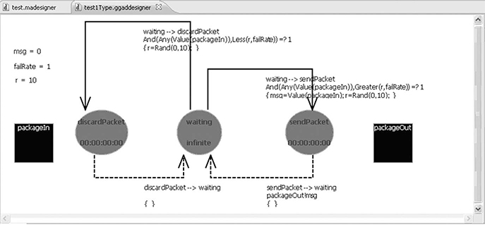
FIGURE 3.1 An atomic model defined as a DEVS graph.
The DEVS graph in Figure 3.1 shows a simple component for a packet routing model. As we can see, there are three states in this DEVS atomic model: waiting, discardPacket, and sendPacket. The model uses two input/output ports (corresponding to the XM and YM sets in the formal specification): packageIn and packetOut. Three variables are defined for this model and initialized: msg, failRate, and r. Internal transitions are shown with dashed arrow lines. The internal transition sendPacket → waiting uses the output function, which is defined to send the value of the variable msg to output port packetOut. The external transitions are shown with solid arrow lines, with a condition that would enable that transition only if it is evaluated to true, and an expression to update some of the model variables (when needed). For instance, the transition from waiting to sendPacket is activated when a packet is received on packageIn (Any(Value(packageIn, 1))) and the failRate is greater than a random value r (Greater(r, failRate)). In that case, the model changes to state send-Packet and also assigns the value of the packet to the msg intermediate variable. It also computes a new random value.
Each DEVS graph is translated into an analytical definition that the runtime engines use to execute. The internal transitions employ the following syntax:
int: source destination [outport!value]* ( { (action;)* } )
Here, source and destination represent the initial and final states associated with the execution of the transition function. As the output function should also execute before the internal transition, an output value can be associated with the internal transition. One or more actions can be triggered during the execution of the transition (changing the values of state variables). External transitions are defined as follows:
ext : source destination ( { (action;)* } )? expression
In this case, when the expression is true (which includes inputs arriving from input ports), the model will change from state source to state destination, while also executing one or more actions. These notations are generated as a direct translation from the graph represented in Figure 3.1.
3.2.1 Difficulties of Devs Formal Verification
DEVS formal definitions for atomic models are the most generic DEVS [3]. The first difficulty in DEVS formal verification, is that model- checking techniques are only decidable for finite state systems. In case of infinite-state systems, irrelevant details must be abstracted to obtain a finite state system before applying model-checking techniques. Another difficulty is the nondeterminism in DEVS behavior. This can be caused by stochastic behavior in a DEVS model due to the use of a probabilistic function in the definition of the external transition function δext or time advance function δint [13]. Another major difficulty in applying automatic formal verification techniques such as model checking to DEVS models is that the DEVS time advance function can take values of irrational real numbers. These values cannot be represented in a finite reachability graph that is used in model-checking algorithms, and thus, the algorithm will not be able to terminate, hence rendering the verification problem undecidable.
Several techniques have been introduced to overcome these problems and provide reasonable approximation to DEVS while enabling formal verification. As will be discussed in the following paragraphs, the techniques range from formal model checking of restricted classes of DEVS, the generation of test traces from DEVS models for simulation testing, the specification of high-level system requirements in TA and verifying DEVS model against those requirements, and introducing clock constructs to DEVS to conform with TA.
One approach, called real-time DEVS (RT-DEVS) introduces a time advance function that maps each state to a range with maximum and minimum time values and introduces an activity associated with every system state [14]. This work also introduced an RT-DEVS executive that executes these models in RT. RT-DEVS was also used to design RT controllers as shown in Ref. [15] for a train-gate system. Further work on verifying RT-DEVS was introduced in Refs. [16,17], where the authors relied on TA as used by UPPAAL and defined (although not formally proved) a transformation method from RT-DEVS to UPPAAL. This transformation allows weak synchronization between components of the TA model as RT-DEVS semantics uses weak synchronization.
Other approaches use a limited version of DEVS that can be verified. For instance, a method based on Finite and Deterministic DEVS (FD-DEVS) was introduced [8] where the time advance function maps states into rational numbers and the external transition function cannot use the elapsed time value. The verification relies on reachability analysis, similar to TA algorithms. FD-DEVS is limited, thus it may not fit some applications that require the full expressiveness of DEVS. Likewise, although reachability analysis algorithms have been defined (and verification is possible), there are no tools available that implement these algorithms.
To avoid these limitations, other approaches tried to map DEVS models to TA [18]. The conversion method mapped a DEVS model through its components and its simulator. The approach suggests trace equivalence as the basis for parallel DEVS and TA model equivalence. This work did not consider some DEVS features that may not map to TA, such as irrational values in DEVS transition functions. Moreover, some limitations also exist for relying on trace equivalence between DEVS and TA, as we will show in Section 3.3. A similar approach presented in Ref. [19] uses TA to specify the high-level system requirements, after which these requirements are modeled as a DEVS model. The system requirements are then verified through simulation of the DEVS model.
The work by Hernandez and Giambiasi [20] showed that the verification of general DEVS models through reachability analysis is undecidable. The authors based their deduction on building a DEVS simulation Turing machine. Since the halting problem in Turing machines is undecidable (i.e., with analysis only, we cannot know in which state a Turing machine would be), they concluded that this is also true for DEVS models. In other words, we cannot recognize if we have reached a particular state starting from an initial state, and consequently, reachability analysis for general DEVS is impossible. Based on this result, reachability analysis may be possible only for restricted classes of DEVS. This result was based on introducing state variables with infinite number of values into the DEVS formalism. Therefore, limiting the number of states of a DEVS model is mandatory for decidable reachability. Hence, further work [21] introduced a new class of DEVS called time-constrained DEVS (TC-DEVS), which expanded the definition of DEVS atomic models with multiple clocks incremented independently of other clocks. Classic DEVS atomic models can be seen as having only one clock that keeps track of the elapsed time in a state and is reset on each transition. TC-DEVS also added clock constraints similar to TA (to function as guards on external and internal transitions). However, it is different from UPPAAL TA in that it allows clock constraints in state invariants to include clock differences. TC-DEVS is then transformed into an UPPAAL TA model. This work, however, did not include a transformation of TC-DEVS state invariants to UPPAAL TA when the model has invariants with clock differences, as this is not allowed in UPPAAL TA.
For large and more complex DEVS models, where formal verification is not feasible, testing would be the only choice. Techniques have been presented to generate testing sequences from model specifications that can then be applied against the model implementation to verify the conformance of the implementation to specifications [22,23].
3.2.2 Rational Time-Advance DEVS
RTA-DEVS was proposed to provide the system modeler with a formalism that is expressive and sufficient to model complex systems behavior, while being verifiable by formal model-checking techniques. RTA-DEVS is a subclass of DEVS that has removed the main difficulties of the formal model verification discussed in Section 3.2.1; yet, it is sufficiently powerful to model complex system behavior.
As in classical DEVS, we must define RTA-DEVS atomic models. The main difference is that RTA-DEVS employs a different definition for the time advance function, ta, and for the external transition function, δext. The Atomic Rational Time-
Advance is defined as follows:
where
X is the set of external inputs.
Y is the set of external outputs.
S is the set of system states.
δint: S → S is the internal transition function (as in classic DEVS).
δext: T × X → S with T = {(s,e)/s 0 ≤ e ≤ ta(s), e ∈ Q0,+∞} is the external transition function (e is the time elapsed since the last transition, which takes a positive rational value).
λ: S → Y ∪ Ø is the output function.
ta: S → Q0,+∞ is the time advance function that maps each state to a positive rational number.
Coupled RTA-DEVS models are defined as in classic DEVS, as discussed in Section 3.2.
A coupled RTA-DEVS model M can be simulated with an equivalent atomic RTA-DEVS model, whose behavior is defined as follows:
where
X and Y are the input and output event sets, respectively. X is the set of all input events accepted and Y is the set of all output events generated by coupled model M.
S = Xi∈D Vi is the model state, expressed as the Cartesian product of all component states, where Vi is the total state for component i, Vi = {(si,tei)| si ∈ Si, tei ∈ [0,ta(si)]}. Here, tei denotes the elapsed time in state si of component i, and Si is the set of states of component i.
s0 = Xi∈D v0i is the initial system state, with v0i = (s0i, 0) the initial state of component i D
ta: S → T is the time advance function. It is calculated for the global state s ∈ S of the coupled model as the minimum time remaining for any state among all components, formally:
ta(s) = min{(ta(sj)−tei) | i ∈ D} where s = (…(si,tei),…) is the global total state of the coupled model at some point in time, si is the state of component i, and tei is elapsed time in that state.
δext: X × V → S is the external transition function for the coupled model, where V is total state of the coupled model, V = {(s,te)| s ∈ S, te ∈ [0,ta(s)]}.
δint: S → S is the internal transition function of the coupled model.
λ: S → Y is the output function of the coupled model.
3.3 DEVS Verification Methodology
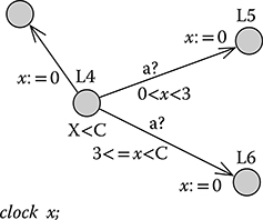
In this section, we introduce our methodology to transform RTA-DEVS models into TA models. The resulting TA models are a subset of deterministic safety automata (which can be used in UPPAAL or other similar model checkers). The transformation methodology can be summarized as follows:
Define a clock variable for each atomic RTA-DEVS model (i.e., x).
Replace every state in RTA-DEVS with a corresponding one in TA (i.e., L1 for source s1 and L2 for destination s2).
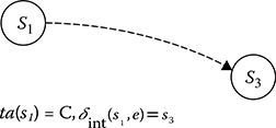
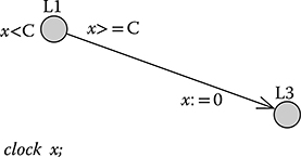
Model the RTA-DEVS internal transition from s1 to s2 as a TA as follows:
For the RTA-DEVS source state s1, define a TA source state L1. For the RTA-DEVS destination state s2, define a TA destination state L2.
Reset the clock variable on the entry to each state (x: = 0).
Put an invariant in the source state derived from the time advance function for that state, that is, x < ta(s1).
Optionally, define a transition with a guard. This guard should be the complement of the invariant in the source state, that is, x ≥ ta(s1).
Define an action for each output function defined.
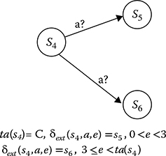
The RTA-DEVS external transition is modeled in TA with the following items:
A source state and some destination state(s), that is, L1 for source s1 and L2 for destination s2.
A clock reset on the entry into each state.
An invariant in the source state that corresponds to the time advance function for that state, that is, x < ta(s1).
For the external transition(s) with guards of clock constraints, these constraints should be disjoint to obtain a deterministic TA model.
The action label on TA transitions for each RTA-DEVS input event to source state s1.
By applying the above-mentioned steps, we obtain a TA model that executes every transition defined in the RTA-DEVS model under study. As already known, the RTA-DEVS behavior is completely defined by its transition functions, which defines all transitions in the RTA-DEVS model. Thus, the resulting TA model executes the RTA-DEVS.
However, TA models cannot have irrational constant values in guards or state invariants. This implies that for any DEVS model containing a state lifetime of irrational values, it will not be possible to directly apply the transformation shown in Table 3.1. In this case, the irrational values would have to be approximated to the nearest rational value according to a choice by the modeler, based on the required precision for the equivalent RTA-DEVS model. In doing so, the transformation should take into account the following rules. These rules avoid building invalid RTA-DEVS or TA models that contain time-action locks (that prevent the model execution progress) or loops where execution progresses infinitely without allowing time to advance [24].
Rule 1: When approximating an irrational value triggering an internal transition that is coupled with an external transition, the choice of approximation value should be consistent for all constants using this irrational number.
TABLE 3.1
Transformation of Rational Time-Advance Devs to Behaviorally Equivalent Time Automata
Rta-Devs |
Equivalent Ta |
Internal transition |
|
|
|
|
External transition |
|
|
|
Formally, assume we have the following defined in a DEVS coupled model as shown in Figure 3.2:
It should be approximated in RTA-DEVS as follows:
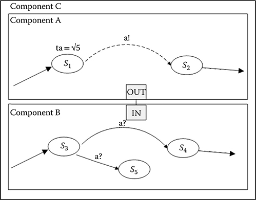
FIGURE 3.2 A coupled DEVS model.
where
Cirr is an irrational real number.
Cr is a rational real number.
, βA, and taA are functions defined for component A.
Rule 2: When approximating an irrational value for elapsed time in the definition of the external transition function, the choice of the approximation value should be consistent for all constants using this irrational number. Formally, assume we have the following DEVS definition of an external transition function in a model similar to the one shown in Figure 3.3:
It should be approximated in the RTA-DEVS model with the following form to avoid creating action locks:
The second rule is to avoid action locks that may happen if we define the external transition function with conditions on its transitions where there is a gap in time (where the function is not defined). Another possibility is to have an approximated external transition function in which conditions on different transitions overlap in time, thus creating nondeterminism that is not in the original DEVS model.
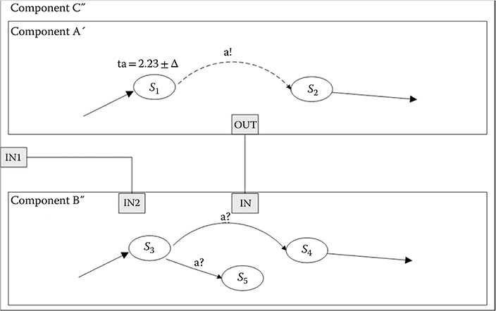
FIGURE 3.3 RTA-DEVS component with external input.
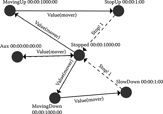
FIGURE 3.4 Elevator RTA-DEVS model.
To further clarify the method, we show a simple example representing the behavior of an elevator [6]. The RTA-DEVS model in Figure 3.4 models the movement of the elevator.
TABLE 3.2
Elevator Model States
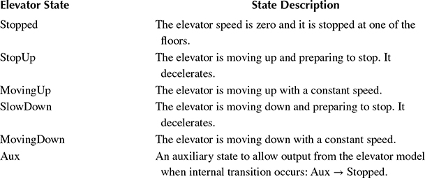
As shown, the elevator can be in one of the five states (listed in Table 3.2).
In this model, the elevator starts in the Stopped state and waits for the controller commands to move to satisfy a button request from the user. The decisions for the proper direction and the start and stop of movement are all taken by the controller. The states of the elevator are represented by circles in the figure. External transitions are enabled when the function Value(mover) evaluates to true. This function is defined as in Table 3.3 for the different transitions shown in Figure 3.4.
Likewise, the behavior of the internal transitions are defined as in Table 3.4.
By following the transformation steps summarized in Table 3.1, we can construct the equivalent TA model as shown in Figure 3.5. This model is constructed to be behaviorally equivalent to the DEVS model of Figure 3.4. This equivalence is essential to ensure that any properties that we must check in the DEVS model are preserved in the constructed TA model.
By applying the methodology we identified in Section 3.3, we go through ther following steps to obtain the TA model in Figure 3.5.
Define a clock variable for each atomic RTA-DEVS model. This results in variable x.
Replace every state in RTA-DEVS with a corresponding one in TA. A location is created for each state in DEVS with the same name as is shown in the TA model.
Model the RTA-DEVS internal transition as a TA as follows.
A source state L1 and a destination state L2: SlowingDown and StopUp states in Figure 3.5 represent source states of SlowDown and StopUp states depicted in Figure 3.4 Reset the clock variable on the entry into each state (x = 0).
Put an invariant in the source state derived from the time advance function for that state. The invariant at both states SlowingDown and StopUp is x < 1.
Optionally, define a transition with a guard. This guard should be the complement to the invariant in the source state. None are defined in this model.
Define an action for each output function that is defined. This corresponds to the two actions stop!1 in the model.
The RTA-DEVS external transition is modeled in TA with the following items.
A source state and some destination state(s). Transitions are defined in the TA model that correspond to the DEVS model.
A clock reset on the entry into each state.
An invariant in the source state that corresponds to the time advance function for that state. This corresponds to the three occurrences of the invariant x < 1000.
For the external transition(s) with guards of clock constraints, these constraints should be disjoint to obtain a deterministic TA model. For example, in the elevator model, direction = =0, direction = = 1, and direction = = 2.
For each event on external transition of the RTA-DEVS model, place a synchronization channel on the corresponding TA transition. For example, the move? and stop! channels in the TA model of Figure 3.5 represent external events of mover(value) and stop!1 in the elevator model of Figure 3.4.
TABLE 3.3
Elevator External Transitions
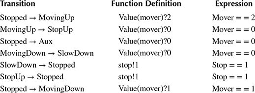
TABLE 3.4
Elevator Internal Transitions
Transition |
Action Definition |
Outport!Value |
SlowingDown → Stopped |
|
stop!1 |
StopUp → Stopped |
|
stop!1 |
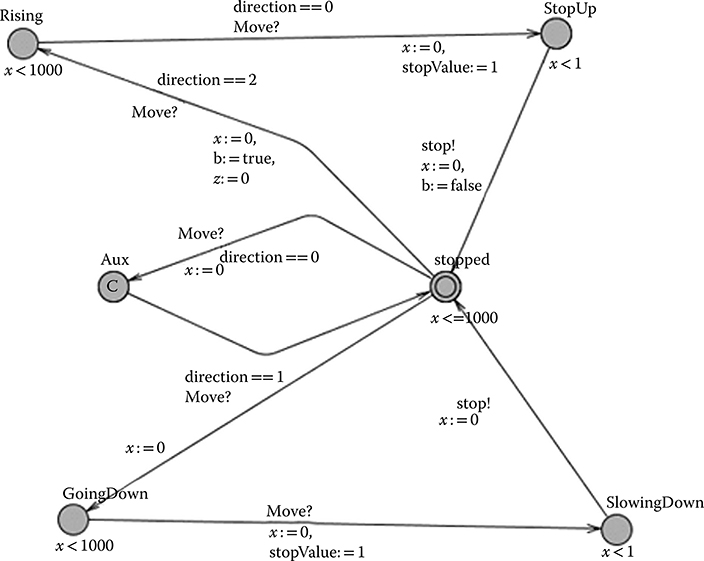
FIGURE 3.5 Elevator timed automata model.
It is important to preserve the equivalence properties also when we map any verification results obtained from the TA model back to the DEVS model. To ensure this equivalence, the transformation from DEVS to TA is done based on the notion of bisimulation equivalence [7]. This equivalence ensures that for each state in DEVS, there is a corresponding one in TA and vice versa. It also ensures that for each transition in DEVS, there would be a corresponding equivalent one in TA and vice versa. Once we have a TA model that is behaviorally equivalent to the DEVS model, any property we wish to verify in the DEVS model can be verified in the TA model, and verification results would apply directly to the DEVS model.
The DEVS Elevator-Controller is shown in Figure 3.6. By applying the transformation steps discussed in the beginning of Section 3.3, we obtain the TA model as shown in Figure 3.7. In this transformation, we represented DEVS states with lifetime of zero as committed locations in the TA model. Examples of these are states Aux1, Stopping, and Moving. Committed locations of TA prevent time to elapse in them and hence serve our purpose for this transformation.
To apply the UPPAAL model checker on this elevator system, the elevator system must be represented as a closed system that allows UPPAAL to explore all its transitions and states. To do so, we define a simple environment model that represents a user requesting the services of the elevator, as shown in Figure 3.8. In this model, the third floor button is pressed after 5 time units. This causes the Elevator-Controller to receive the floor value and then send the corresponding command to the elevator model to reach the third floor. The environment model then simulates different user requests.

FIGURE 3.6 Elevator controller model as a DEVS graph.
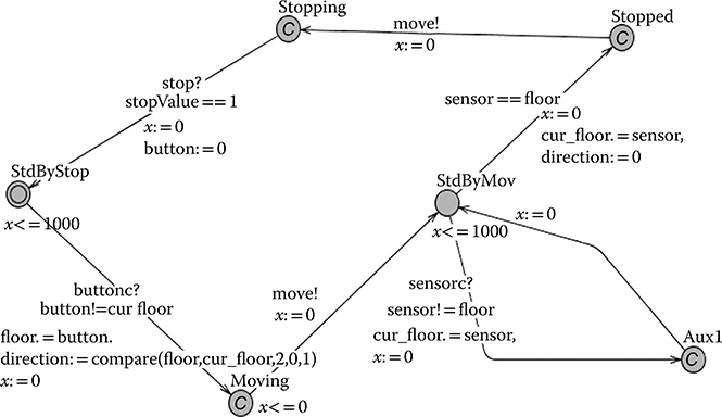
FIGURE 3.7 Timed automata controller model in UPPAAL.
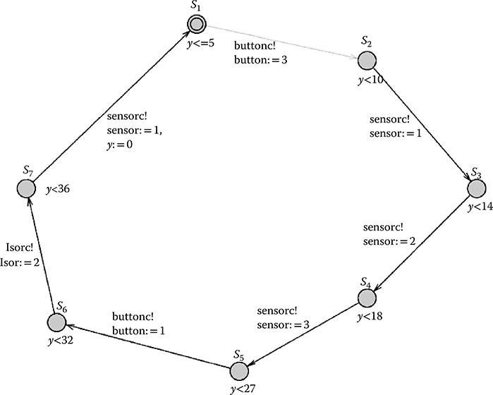
FIGURE 3.8 Environment inputs (button and sensor).
The system composed of the Elevator, the Elevator-Controller, and the Environment can be checked using UPPAAL to verify certain properties about the system. For instance, some of the important properties would be as follows:
Does the DEVS model progress? Can we detect deadlock conditions?
If no deadlocks are found, is it always guaranteed whenever a user pushes a floor button that the elevator would reach that floor (i.e., the normal operation of the elevator system)?
If the elevator eventually reaches the floor, is there a guaranteed upper bound between the request and the arrival of the elevator?
For the first question, we applied UPPAAL to our model to check for any deadlocks that may be present in the elevator. To check for that failure, we had formulated a simple query, expressed in computational tree logic (CTL) [25, 26 and 27] as follows:
A[] not deadlock
After running the checker, it shows that this property is satisfied, that is, there is no deadlock, as shown in Figure 3.9.
The property (b) is an example of the system liveness, in which we are interested to check if by pressing a certain floor button, the elevator would eventually reach that floor. For example, if the user presses the third-floor button, the elevator should eventually reach the third floor. This property is expressed in CTL as follows:

FIGURE 3.9 Elevator verification results in UPPAAL.
button = = 3 --> ElevatorController.cur_floor = = 3
This states that whenever a user input for the third-floor button occurs, the cur_floor variable in the ElevatorController would eventually reach that floor. This property was also satisfied in UPPAAL model checker for the given model.
To check the third property (c), that is, whether the elevator would reach the requested third floor within some bounded time, we extend the model for bounded time checking by adding the Boolean variable b and a global clock z as shown in the elevator model in Figure 3.5. The variable b would be set to true for the time when the elevator starts traveling up until it reaches the Stopped state again. Therefore, by checking the accumulated time while b is true, it would provide us the property we must check. Then, the property can be expressed with the following query:
A[] ( b imply z < 27 ) which is satisfied.
However, the query
A[] ( b imply z < 26 ) is not satisfied.
This shows that the elevator would reach the third floor after requested to go there after no less than 26 time units, but is guaranteed to be there after 27 time units or more.
3.4 Case Study: Controller for an E-Puck Robotic Application
In this section, we present a case study where we use DEVS to build a model of a controller for an E-puck robot and later the same model is used as an actual controller. The E-puck (shown in Figure 3.10) is a desktop-size mobile robot with a wide range of possibilities (signal processing, autonomous control, embedded programming, etc.).
The E-puck contains various sensors covering different modalities: (i) eight infrared (IR) proximity sensors placed around the body measure the closeness of obstacles, (ii) a 3D accelerometer provides the acceleration vector of the E-puck, (iii) three microphones to capture sound, and (iv) a color CMOS (Complementary Metal Oxide Semiconductor) camera with a resolution of 640 × 480 pixels. It also includes the following actuators: (i) two stepper motors, making it capable of moving forward and backward, and spinning in both directions; (ii) a speaker, connected to an audio codec; (iii) eight red light-emitting diodes (LED) placed all around the top; and (iv) a red front LED placed beside the camera.
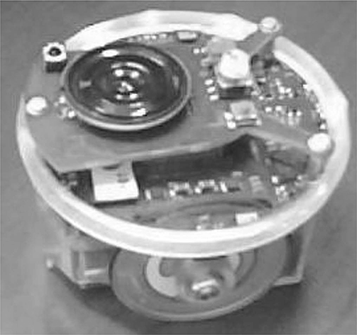
FIGURE 3.10 E-puck robot.
In the following sections, we introduce a DEVS model for a simple controller for the E-puck, the corresponding implementation in CD++, and the formal verification of different properties of the model through the transformation introduced in Section 3.4 combined with the use of the UPPAL model checker.
3.4.1 DEVS Model Specification
The controller is designed to steer the robot in a field while avoiding obstacles. We have defined a DEVS model with an atomic component (epuck0) that imitates the behavior of the controller, shown in Figure 3.11. There are eight input ports (InIR0, … InIR7), each of them modeling the connection to one proximity sensor. The input ports periodically receive the distances to the obstacles from the sensors. There are also two output ports: OutMotor, which transfers the output commands to the motors, and OutLED, to turn on/off the LEDs.
The controller can command the following actions based on the inputs received from the sensors: move forward, turn 45 degrees left, turn 45 degrees right, turn 90 degrees left, turn 90 degrees right, turn 180 degrees, and stop. Initially, the robot starts moving forward while receiving the periodic inputs from proximity sensors and analyzing them. As soon as it detects an obstacle, it performs one of the turning actions based on the position of the obstacle. The robot continues turning until it finds an empty space ahead. The controller also uses LEDs to signal the action that is being performed. For example, if the robot is moving forward, the front LED (led0) turns on and if it is turning 45 degrees to the left, led7 turns on. Figure 3.12 illustrates two sample imaginary scenarios in which obstacles block the robot’s path.
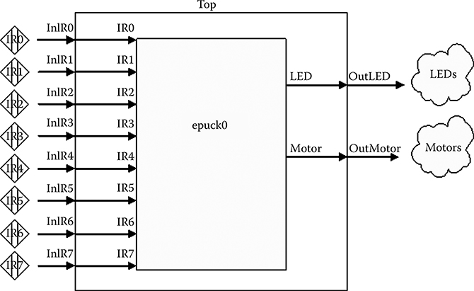
FIGURE 3.11 E-puck controller DEVS model hierarchy.
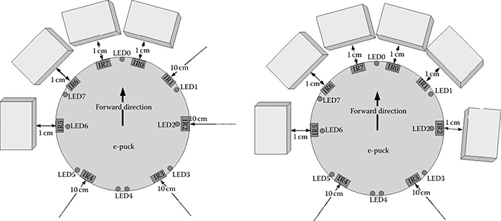
FIGURE 3.12 (a) Scenario 1: front-left blocked. (b) Scenario 2: front completely blocked.
The DEVS formal specification of the epuck0 atomic component is as follows:
where
X = {(IR0, R), (IR1, R), (IR2, R), (IR3, R), (IR4, R), (IR5, R), (IR6, R), (IR7, R)}.
S = {move forward, turn 45° left, turn 45° right, turn 90° left, turn 90° right, turn 180°, stop, prepare move forward, prepare turn 45° left, prepare turn 45° right, prepare turn 90° left, prepare turn 90° right, prepare turn 180°, prepare stop}.
Y = {(LED, (100, 0, 10, 20, …, 70, 1, 11, 21, …, 71)), (Motor, (0, 1, …, 6))}.
δext = If there is an obstacle trigger the proper state change based on Figure 3.13.
δint = Change the state based on Figure 3.13.
λ = Generate appropriate outputs to the robot based on Figure 3.13.
ta = move forward → ∞; turn 45° left → 100 milliseconds; turn 45° right → 100 milliseconds; turn 90° left → 200 milliseconds; turn 90° right → 200 milliseconds; turn 180° → 400 milliseconds; stop → ∞; prepare move forward → 0 second; prepare turn 45° left → 0 second; prepare turn 45° right → 0 second; prepare turn 90° left → 0 second; prepare turn 90° right → 0 second; prepare turn 180° → 0 second; prepare stop → 0 second.
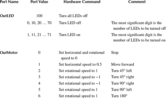
Table 3.5 summarizes the integer outputs of the DEVS model and their associated actions to be performed in the robot hardware. The driver interface programmed by the user transforms the numeric values to actions in the robot.
Figure 3.13 illustrates an abstract state diagram of the epuck0 atomic component. The DEVS graph state diagram summarizes the behavior of a DEVS atomic component by representing the states, transitions, inputs, outputs, and state durations graphically. As we can see, initially, the robot moves forward and if no obstacle is detected from IR0, IR1, IR6, and IR7 (the four sensors scanning the front direction, as seen in Figure 3.12), it continues moving forward. As soon as an obstacle is detected, the value of the sensor IR6 is examined. If this sensor shows no obstacle, the left corner of the robot is open resulting in a 45° turn toward the left. Otherwise, it checks IR1, and if there is space, the robot turns 45° to the right. If both IR1 and IR6 are blocked, the controller examines IR2; if there is space, the robot performs a 90° turn to the left. The same occurs with IR2. If all sensors are blocked, the robot tries turning to the opposite direction (180°).
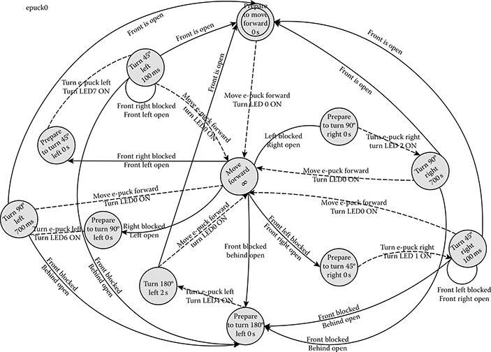
FIGURE 3.13 epuck0 atomic component state diagram.
TABLE 3.5
Devs Output Mapping Table
3.4.2 Implementation on the ECD++ Toolkit
To program a DEVS model on ECD++ [28,10], three main components are necessary.
A model file in which the model hierarchy, model components, input and output ports of each component and input/output couplings are declared. The model file is passed to the ECD++ executable file as a runtime argument, and the latter instantiates the model components based on the declarations in the model file.
Source files of the model components. For each atomic component, a C++ class is defined, and the external and internal transitions and the output function are programmed as methods of this class.
A driver interface. A driver function is overridden by the user for each input or output port at the top level of the model hierarchy that is connected to a hardware counterpart.
The ECD++ model file also contains information about the period of the input drivers and the duration of the states for each atomic component. In this example, we have tuned the input period of the IR sensors to 50 milliseconds. Therefore, for every 50 milliseconds, the external transition of the epuck0 atomic component is invoked, and based on the updated values, the next action is decided. The following is the ECD++ model file of the e-puck robot controller model.
1 [top]
2 components : epuck0@epuck
3 out : outmotor outled
4 in : inir0 inir1 inir2 inir3 inir4 inir5 inir6 inir7 5 link : inir0 ir0@epuck0
6 link : inir1 ir1@epuck0
7 link : inir2 ir2@epuck0
8 link : inir3 ir3@epuck0
9 link : inir4 ir4@epuck0
10 link : inir5 ir5@epuck0
11 link : inir6 ir6@epuck0
12 link : inir7 ir7@epuck0
13 link : motor@epuck0 outmotor
14 link : led@epuck0 outled
15 inir0 : 00:00:00:100
16 inir1 : 00:00:00:100
17 inir2 : 00:00:00:100
18 inir3 : 00:00:00:100
19 inir4 : 00:00:00:100
20 inir5 : 00:00:00:100
21 inir6 : 00:00:00:100
22 inir7 : 00:00:00:100
23
24 [epuck0]
25 preparationTime : 00:00:00:000
26 turn45Time : 00:00:00:100
27 turn90Time : 00:00:00:700
28 turn180Time : 00:00:02:000
Line 1 defines the top coupled component and line 2 declares its components. Lines 3 and 4 declare the output and input ports within the top coupled component, respectively. Lines 6–14 define the internal couplings. Lines 15–22 declare the periods of each input port. Lines 24–27 declare the duration of states within the epuck0 component.
The external function performs the state transitions based on the DEVS graph diagram presented in Section 3.4.1. The following is the source code of the external transition function of epuck0 atomic component.
1 if(state!=Mov_Fwd && IR0>0.04 && IR7>0.04 && IR1>0.02 && IR6>0.02){
2 }else if((state==Mov_Fwd)&&(IR0<0.05 || IR1< 0.02) && IR6>0.04){
3 state = Pre_Trn_45_Lft;
4 holdIn( Atomic::active, preparationTime );
5 }else if((state==Trn_45_Lft)&&(IR0<0.05 || IR1<0.02) && IR6>0.04){
6 state = Trn_45_Lft;
7 holdIn( Atomic::active, turn45Time);
8 }else if((state == Mov_Fwd)&& (IR6< 0.02 || IR7< 0.05) && IR1> 0.04){
9 state = Pre_Trn_45_Rgt;
10 holdIn( Atomic::active, preparationTime);
11 }else if((state==Trn_45_Rgt)&& (IR6< 0.02 || IR7< 0.05) && IR1> 0.04){
12 state = Trn_45_Rgt;
13 holdIn( Atomic::active, turn45Time);
14 }else if(state == Mov_Fwd && IR[0]< 0.05 && IR[7]< 0.05 && IR[2]> 0.04){
15 state = Pre_Trn_90_Lft;
16 holdIn( Atomic::active, preparationTime);
17 }else if(state == Mov_Fwd && IR[0]< 0.05 && IR[7]< 0.05 && IR[5]> 0.04){
18 state = Pre_Trn_90_Rgt;
19 holdIn(Atomic::active, preparationTime);
20 }else if(state!=Trn_180&&IR[0]<0.05&&IR[7]<0.05&&IR[2]<0.05 &&IR[5]<0.05){
21 state = Pre_Trn_180;
22 holdIn( Atomic::active, preparationTime);
23 }
Line 1 shows the case when moving forward is the current state and there is no obstacle ahead. Line 2 manages the case when IR0 or IR1 (right side of the robot) is obstructed. In that case, the state of the robot is changed to prepare turn 45° left (line 3), and in line 4, the time duration of this state is set. The other cases and the state changes are also indicated in the above-mentioned code snippet. The internal transition function and the output function are similar. For instance, the following code snippet shows a part of the internal transition function:
1 Model &epuck::internalFunction( const InternalMessage & )
2 {
3 switch (state){
4 case Pre_Mov_Fwd:
5 case Trn_45_Lft:
6 case Trn_45_Rgt:
7 case Trn_90_Lft:
8 case Trn_90_Rgt:
9 case Trn_180:
10 state = Mov_Fwd ;
11 passivate();
12 break;
13
14 case Pre_Trn_45_Lft:
15 state = Trn_45_Lft ;
16 holdIn( Atomic::active, turn45Time );
17 break;
18 …
Lines 4–9 show a part of the internal transition for the states prepare move forward, turn 45° left, turn 45° right, turn 90° left, turn 90° right, and turn 180°, after which the model continues to move forward (line 10). Line 14 shows the case for prepare turn 45° left state, after which the component transfers to turn 45° left state.
The following code snippet shows a part of the ECD++ output function (λ) implementation:
1 Model &epuck::outputFunction( const InternalMessage &msg )
2 {
3 switch (state){
4 case Pre_Mov_Fwd:
5 sendOutput( msg.time(), led, 100) ;//Turn all Leds off
6 sendOutput( msg.time(), motor, 1) ;//Moving Forward
7 sendOutput( msg.time(), led, 1) ;//Turn Led 0 on 8 break;
9
10 case Trn_45_Lft:
11 sendOutput( msg.time(), led, 70) ;//Turn Led 7 off
12 sendOutput( msg.time(), motor, 1) ;//Moving Forward
13 sendOutput( msg.time(), led, 1) ;//Turn Led 0 on 14 break;
15 …
In this case, line 4 handles the outputs of state prepare move forward in which three different outputs are generated. Line 5 is the output command to turn off all LEDs. Line 6 shows the moving forward command sent to the motor port and line 7 is the command to turn led0 on. These outputs are then decoded and converted by the corresponding drivers. Lines 9–13 show the outputs for the turn 45° left state where the led7 is turned off first, then the motors are instructed to move forward and led0 is turned on afterwards.
The following code snippet shows the driver interface function for the OutMotor output port of the top coupled component. The outputs generated in the output function for the motor port of the epuck0 atomic component are inputted to this function as an integer argument and the respective hardware command is spawned here.
1 bool OutMotor::pDriver(Value &value)
2 {
3 switch((int)value){
4 case 0: //Stop
5 playerc_position2d_set_cmd_vel(position2d, 0, 0, 0, 1);
6 break;
7 case 1: //Moving Forward
8 playerc_position2d_set_cmd_vel(position2d, 1, 0, 0, 1);
9 break;
10 case 3: //Turn 45 deg. Right
11 case 4: //Turn 90 deg. Right
12 playerc_position2d_set_cmd_vel(position2d, 0,0,-10,1);
13 break;
14 case 2: //Turn 45 deg. Left
15 case 5: //Turn 90 deg. Left
16 case 6: //Turn 180 deg. (turn from left)
17 playerc_position2d_set_cmd_vel(position2d, 0, 0, 10,1);
18 break;
19 };
20 }
Lines 4–6 show the case of the stop command, which is encoded with value 0. Line 5 is the command to stop the robot. Lines 7–9 handle the moving forward output command and lines 10–13 manage the right turning commands. For both 45° and 90° turn actions, the robot starts spinning to the right, while the calibrated duration of the respective state accomplishes the desired degree of spinning. A more accurate approach to perform the turning actions would measure the spinning angle constantly and stop when the desired angle is reached.
3.4.3 Executing the Models
The e-puck model was first tested using virtual-time simulation mode. We designed a virtual space with obstacles and ran the simulation with inputs supplied from an event file, in which two series of inputs to the sensors are defined. Figure 3.14 shows the contents of the event file and output file of the ECD++ and the action associated with the outputs of the controller model. The event file is structured in the format of “time, input port and value” and in this example it consists of two series of events representing the two scenarios shown in Figure 3.12. The first three lines of the output file are the initial outputs of the model that move the robot forward. After 4 seconds of simulation, the first series of inputs is injected into the model, which results in the second series of outputs. The latter spins the robot 45° to the right and performs the appropriate LED commands and after 100 milliseconds moves the robot forward again with the appropriate LED commands. A similar scenario happens for the second series of inputs at time 8 of simulation in which the robot turns 180°.
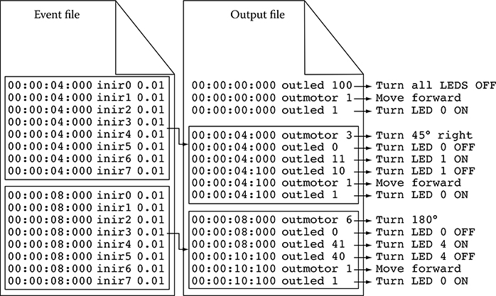
FIGURE 3.14 Event file and output file of ECD++.
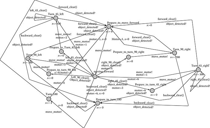
FIGURE 3.15 Robot controller timed automata model.
After verifying the behavior of the model in various scenarios, we tested the model using the actual e-puck robot. The model was executed in RT mode in which the model interacts with the target platform (in this case, the robot hardware). The same behavior was observed and the robot found its way through the obstacles.*
3.4.4 Verifying the Model
To obtain a TA model that is behaviorally equivalent to the DEVS model shown in Figure 3.13, we followed the procedure discussed in Sections 3.3 and 3.4. The equivalent TA is shown in Figure 3.15. In this model, the Boolean conditions of the DEVS state model were defined in functions in the TA model as shown in the following code snippet.
* The results can be seen at http://youtube.com/arslab.
1 bool forward_clear(){return ir0>4 && ir7 >4 && ir1>2 && ir6>2;}
2 bool left_45_clear(){return (ir0<5 || ir1<2) && ir6>4;}
3 bool right_45_clear(){return (ir6>2 || ir7 <5) && ir1>4;} 4 bool backward_clear(){return ir0<5 && ir7 <5 && ir2<5 && ir5<5;}
5 bool right_90_clear(){return ir0<5 && ir7 <5 && ir5>4;}
6 bool left_90_clear(){return ir0<5 && ir7 <5 && ir2>4;}
In this TA model, Boolean functions constitute guards on the transitions that evaluate to true whenever the sensor values satisfy the condition given in the DEVS model. While the DEVS model of the robot-controller was tested and simulated with the real robot moving in a specific environment, to verify the robot-controller model, we built a closed system where this model interacts with other models representing the motor and the environment in which the robot travels.
Figure 3.16 shows the TA model of the motor. This model represents the motor states, starting in Preparing_To_Move_Forward. It then synchronizes the motor model with the controller model through the move_motor channel. The motor model shows six states that the motor can visit depending on the value of the shared variable motor, which is updated by the Robot Controller model.
In Figure 3.17, a simple model of the environment in which the robot may travel is shown. This model represents an environment that looks like a contoured closed layout. This layout was modeled in TA by the values assigned to different sensors on the robot ir0, ir1, … , ir7. These values are also shown in the event file used to test the robot DEVS model.
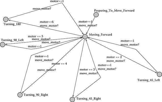
FIGURE 3.16 Motor timed automata model.
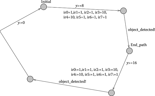
FIGURE 3.17 Environment timed automata model.
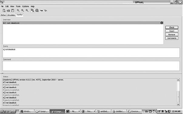
FIGURE 3.18 UPPAAL verification for deadlocks.
The verification of the system composed of Robot-Controller, Motor, and Environment in the UPPAAL tool revealed that it is free of deadlocks as shown in Figure 3.18. This ensures the controller is always able to successfully guide the robot through the given layout.
More complex layouts can also be modeled in TA to verify the system for more complicated behavior. For example, the TA environment model could be constructed to randomly assign values in reasonable range to the sensors. This would model generating arbitrary shaped obstacles around the robot. The verification for deadlock would then be executed to reveal if a deadlock is possible at any particular shape facing the robot. This would reveal either a fault in the robot-controller or the controller being too simple to handle irregular shapes facing the robot.
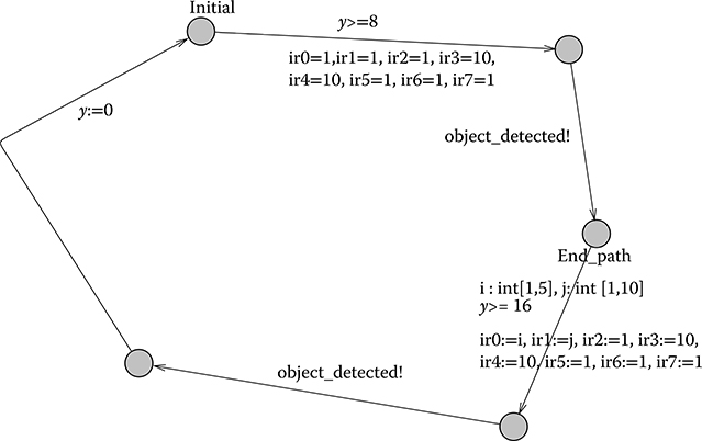
FIGURE 3.19 Environment model with random sensor inputs.
Another example of verification that we can explore with verification includes different kinds of environments for the robot controller. In this example, we would attempt to check if the controller may enter into a deadlock and stop progress. To do so, we modify the environment model to randomly generate different sensor readings that simulate the robot approach to the situation where there is variety in the environment. This modified environment model is shown in Figure 3.19. In this model, sensor ir0 obtains a value in the range of [1,5], ir1 a value in [1,10].
By checking the model for deadlock again, the UPPAAL tool would verify this property and give a trace if this property is violated. The trace comprises values shown in the following lines.
1 motor = 1
2 ir0 = 5
3 ir1 = 1
4 ir2 = 1
5 ir3 = 10
6 ir4 = 10
7 ir5 = 1
8 ir6 = 1
9 ir7 = 1
This shows that the current design for the robot controller would not handle this combination of sensor values. In this case, either the designer reevaluates the design to address the shortcoming or it may be stated as an assumption on the simple robot controller that this shortcoming is acceptable.
3.5 Conclusions
Mixing formal software verification and validation together with simulation techniques provides a strong methodology for simulation models verification and validation models. Because it is amenable to RT simulation, this methodology constitutes a significant contribution to the field of embedded software engineering. Simulation models must be validated against actual system properties to make sure the modeler captured the essence of the system under study. Formal verification provides this assurance without the need to run exhaustive simulations and manually analyze simulation results. Simulation models also must be verified against any errors that may have been introduced during model building. Errors such as infinite transitions in a bounded time, which result in an illegitimate DEVS model, are difficult to debug manually and thus good candidates for formal verification.
Embedded systems design must model both the physical system under control and the controller. These models hold more value if they are written in a formalism that can be simulated, such as is the case for DEVS. This allows the designer to simulate the system, change design, and simulate again to reach a correct and optimal design. Formal verification helps verify absence of defects in the system. Once the system is proven to be free of defects, the controller DEVS model, being verified within the complete system, is deployed as the executable controller by running on an embedded DEVS simulator. This eliminates any transformation between the verified model and its implementation, thus avoiding potential defects from creeping into the final implementation because of necessary transformations.
References
1. Merz, S., and N. Navet. 2008. Modeling and Verification of Real-Time Systems: Formalisms and Software Tools. Hoboken, NJ: John Wiley & Sons, Inc.
2. Wainer, G., E. Glinsky, and P. MacSween. 2005. “A Model-Driven Technique for Development of Embedded Systems based on the DEVS Formalism.” In Model-Driven Software Development. Volume II of Research and Practice in Software Engineering, edited by S. Beydeda and V. Gruhn. Berlin, Heidelberg: Springer-Verlag.
3. Zeigler, B. P., H. Praehofer, and T. G. Kim. 2000. Theory of Modeling and Simulation. 2nd ed. New York: Academic Press.
4. Alur, R., and D. Dill. 1994. “Theory of Timed Automata.” Theoretical Computer Science 126: 183–235.
5. Miller, J. 2000. “Decidability and Complexity Results for Timed Automata and Semi-linear Hybrid Automata.” In Hybrid Systems: Computation and Control, LNCS 1790, pp. 296–309, London, UK: Springer-Verlag.
6. Saadawi, H., and G. Wainer. 2009. “Verification of Real-Time DEVS Models.” In Proceedings of DEVS Symposium 2009, pp. 143:1–143:8, San Diego, CA: Society for Computer Simulation International.
7. Saadawi, H., and G. Wainer. 2010. “Rational Time-Advance DEVS (RTA-DEVS).” In Proceedings of DEVS Symposium 2010, Orlando, FL, pp. 143:1–143:8, San Diego, CA: Society for Computer Simulation International.
8. Hwang, M-H., and B. P. Zeigler. July 2009. “Reachability Graph of Finite and Deterministic DEVS Networks.” IEEE Transactions on Automation Science and Engineering 6 (3): 468–78.
9. Behrmann, G., A. David, and K. Larsen. 2004. “A Tutorial on Uppaal.” In Proceedings of the 4th International School on Formal Methods for the Design of Computer, Communication, and Software Systems, LNCS, 3185, pp. 200–237, Springer-Verlag.
10. Wainer. G. 2009. Discrete-Event Modeling and Simulation: A Practitioner’s Approach. Boca Raton, FL: CRC Press, Taylor & Francis.
11. Zeigler, B. P., H. Song, T. Kim, and H. Praehofer. 1995. “DEVS Framework for Modelling, Simulation, Analysis, and Design of Hybrid Systems.” In Proceedings of HSAC, Ithaca, NY, LNCS 999, pp. 529–551, London, UK: Springer-Verlag .
12. Christen, G., A. Dobniewski, and G. Wainer. 2004. “Modeling State-Based DEVS Models in CD++.” In Proceedings of MGA, Advanced Simulation Technologies Conference, Arlington, VA. San Diego, CA: Society for Computer Simulation International.
13. Castro, R., E. Kofman, and G. Wainer. 2010. “A Formal Framework for Stochastic DEVS Modeling and Simulation.” Simulation, Transactions of the SCS 86 (10): 587–611.
14. Hong, J. S., H. S. Song, T. G. Kim, and K. H. Park. 1997. “A Real-Time Discrete Event System Specification Formalism for Seamless Real-Time Software Development.” Discrete Event Dynamic Systems 7 (4): 355–75.
15. Song, H. S., and T. G. Kim. February 2005. “Application of Real-Time DEVS to Analysis of Safety-Critical Embedded Control Systems: Railroad Crossing Control Example.” Simulation 81 (2): 119–36.
16. Furfaro, A., and L. Nigro. 2008. “Embedded Control Systems Design Based on RT-DEVS and Temporal Analysis using UPPAAL.” In Computer Science and Information Technology, IMCSIT 2008, October 20–22, 2008, pp. 601–08, Polish Information Processing Society.
17. Furfaro, A., and L. Nigro. June 2009. “A Development Methodology for Embedded Systems Based on RT-DEVS.” Innovations in Systems and Software Engineering 5: 117–27.
18. Han, S., and K. Huang. 2007. “Equivalent Semantic Translation from Parallel DEVS Models to Time Automata”. In Proceedings of 7th International Conference on Computational Science, ICCS, pp. 1246–1253, Berlin, Heidelberg: Springer-Verlag.
19. Giambiasi, N., J.-L. Paillet, and F. Châne. 2003. “Simulation and Verification II: From Timed Automata to DEVS Models.” In Proceedings of the 35th Winter Simulation Conference (WSC ‘03), New Orleans, LA, pp. 923–931, San Diego, CA: Society for Computer Simulation International.
20. Hernandez, A., and N. Giambiasi. 2005, pp. 923–931, San Diego, CA: Society for Computer Simulation International. “State Reachability for DEVS Models.” In Proceedings of Argentine Symposium on Software Engineering, Buenos Aires, Argentina, pp. 251–265.
21. Dacharry, H., and N. Giambiasi. 2007. “Formal Verification Approaches for DEVS.” In Proceedings of the 2007 Summer Computer Simulation Conference (SCSC), San Diego, CA, pp. 312–319, San Diego, CA: Society for Computer Simulation International.
22. Hong, K. J., and T. G. Kim. 2005. “Timed I/O Test Sequences for Discrete Event Model Verification.” In AIS 2004, Jeju, Korea, pp. 275–84, LNAI 3397.
23. Labiche, Y., and G. Wainer. 2005. “Towards the Verification and Validation of DEVS Models.” In Proceedings of the 1st Open International Conference on Modeling & Simulation, Clermont-Ferrand, France, pp. 295–305.
24. Bowman, H., and R. Gomez. 2006. Concurrency Theory: Calculi and Automata for Modelling Untimed and Timed Concurrent Systems. London: Springer-Verlag.
25. Emerson, E. A., and E. M. Clarke. 1982. “Using Branching-Time Temporal Logic to Synthesize Synchronization Skeletons.” Science of Computer Programming 2 (3): 241–66.
26. Alur, R., C. Courcoubetis, and D. L. Dill. 1990. “Model-Checking for Real-Time Systems.” In 5th Symposium on Logic in Computer Science (LICS’90), pp. 414–25, IEEE.
27. Henzinger, T. A. 1994. “Symbolic Model Checking for Real-Time Systems.” Information and Computation 111: 193–244.
28. Moallemi, M., and G. Wainer. 2010. “Designing an Interface for Real-Time and Embedded DEVS.” In Proceedings of 2010 Symposium on Theory of Modeling and Simulation, TMS/DEVS’10, Orlando, FL.Transition, pp. 137.1–137.8, San Diego, CA: Society for Computer Simulation International.