Compressing Data Files
Overview
By
default, a SAS data file is uncompressed. You can compress your data
files in order to conserve disk space, although some files are not
good candidates for compression. The file structure of a compressed
data file is different from the structure of an uncompressed file.
You use the COMPRESS= data set option or system option to compress
a data file. You use the POINTOBS= data set option to enable SAS to
access observations in compressed files directly rather than sequentially.
You use the REUSE= data set option or system option to specify that
SAS should reuse space in a compressed file when observations are
added or updated.
Review of Uncompressed Data File Structure
By
default, a SAS data file is not compressed. In uncompressed data files,
the following statements are true:
-
Each data value of a particular variable occupies the same number of bytes as any other data value of that variable.
-
Each observation occupies the same number of bytes as any other observation.
-
Character values are padded with blanks.
-
Numeric values are padded with binary zeros.
-
There is a 1-bit per observation overhead (rounded up to the nearest byte) at the end of each page; this bit denotes an observation's status as deleted or not deleted.
-
New observations are added at the end of the file. If a new observation does not fit on the current last page of the file, a whole new data set page is added.
-
The descriptor portion of the data file is stored at the end of the first page of the file.
The figure below depicts
the structure of an uncompressed data file.
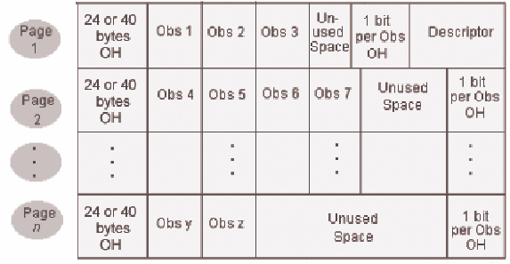
Note: In a 64–bit operating
environment, each page has a 40–byte overhead. In a 32–bit
operating environment, each page has a 24–byte overhead.
In comparison, look
at the characteristics of a compressed data file.
Compressed Data File Structure
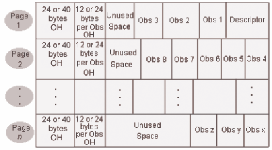
In
compressed data files, the following statements are true:
-
An observation is treated as a single string of bytes by ignoring variable types and boundaries.
-
Consecutive repeating characters and numbers are collapsed into fewer bytes.
-
There is a 24-byte overhead at the beginning of each page in a 32–bit operating environment or 40–byte overhead in a 64–bit operating environment.
-
There is a 12-byte- or 24-byte-per-observation overhead following the page overhead. This space is used for deletion status, compressed length, pointers, and flags.
Each observation in
a compressed data file can have a different length, which means that
some pages in the data file can store more observations than others
can. When an updated observation is larger than its original size,
it is stored on the same data file page and uses available space.
If not enough space is available on the original page, the observation
is stored on the next page that has enough space, and a pointer is
stored on the original page.
The figure below depicts
the structure of a compressed data file.
Deciding Whether to Compress a Data File
Not
all data files are good candidates for compression. Remember that
in order for SAS to read a compressed file, each observation must
be uncompressed. This requires more CPU resources than reading an
uncompressed file. However, compression can be beneficial when the
data file has one or more of the following properties:
-
It is large.
-
It contains many long character values.
-
It contains many values that have repeated characters or binary zeros.
-
It contains many missing values.
-
It contains repeated values in variables that are physically stored next to one another.
In
character data, the most frequently encountered repeated value is
the blank. Long text fields, such as comments and addresses, often
contain repeated blanks. Likewise, binary zeros are used to pad numeric
values that can be stored in fewer bytes. This happens most often
when you assign a small or medium-sized integer to an 8-byte numeric
variable.
Note: If saving disk space is crucial,
consider storing missing data as a small integer, such as 0 or 9,
rather than as a SAS missing value. Small integers can be compressed
more than SAS missing values can.
A data file is not a
good candidate for compression if it has any of the following characteristics:
-
few repeated characters
-
small physical size
-
few missing values
-
short text strings
The following topic
explores how to compress a data file.
The COMPRESS= System Option and the COMPRESS= Data Set Option
To compress a data file, you use
either the COMPRESS= data set option or the COMPRESS= system option.
You use the COMPRESS= system option to compress all data files that
you create during a SAS session. Similarly, you use the COMPRESS=
data set option to compress an individual data file.
|
General form, COMPRESS=
system option:
OPTIONS COMPRESS= NO | YES | CHAR | BINARY;
NO
is the default setting,
which does not compress the data set.
CHAR or YES
uses the Run Length
Encoding (RLE) compression algorithm, which compresses repeating consecutive
bytes such as trailing blanks or repeated zeros.
BINARY
uses Ross Data Compression
(RDC), which combines run-length encoding and sliding-window compression.
|
Note: If you set the COMPRESS=
system option to a value other than NO, SAS compresses every data
set that is created during the current SAS session, including temporary
data sets in the Work library. Although this might conserve data storage
space, it uses greater amounts of other resources.
|
General form, COMPRESS=
data set option:
DATA SAS-data-set (COMPRESS=
NO | YES | CHAR | BINARY);
SAS-data-set
specifies the data
set that you want to compress.
NO
is the default setting,
which does not compress the data set.
CHAR or YES
uses the Run Length
Encoding (RLE) compression algorithm, which compresses repeating consecutive
bytes such as trailing blanks or repeated zeros.
BINARY
uses Ross Data Compression
(RDC), which combines run-length encoding and sliding-window compression.
|
Note: The COMPRESS= data set option
overrides the COMPRESS= system option.
The YES or CHAR setting
for the COMPRESS= option uses the RLE compression algorithm. RLE compresses
observations by reducing repeated consecutive characters (including
blanks) to two-byte or three-byte representations. Therefore, RLE
is most often useful for character data that contains repeated blanks.
The YES or CHAR setting is also good for compressing numeric data
in which most of the values are zero.
The BINARY setting for
the COMPRESS= option uses RDC, which combines run-length encoding
and sliding-window compression. This method is highly effective for
compressing medium to large blocks of binary data (numeric variables).
A file that has been
compressed using the BINARY setting of the COMPRESS= option takes
significantly more CPU time to uncompress than a file that was compressed
with the YES or CHAR setting. BINARY is more efficient with observations
that are several hundred bytes or more in length. BINARY can also
be very effective with character data that contains patterns rather
than simple repetitions.
When
you create a compressed data file, SAS compares the size of the compressed
file to the size of the uncompressed file of the same page size. Then
SAS writes a note to the log indicating the size reduction percent
that is obtained by compressing the file.
When you use either
of the COMPRESS= options, SAS calculates the size of the overhead
that is introduced by compression as well as the maximum size of an
observation in the data set that you are attempting to compress. If
the maximum size of the observation is smaller than the overhead that
is introduced by compression, SAS disables compression, creates an
uncompressed data set, and issues a warning message stating that the
file was not compressed.
Once a file is compressed,
the setting is a permanent attribute of the file. In order to change
the setting to uncompressed, you must re-create the file.
Note: Compression of observations
is not supported by all SAS engines. See the SAS documentation for
the COMPRESS= data set option for more information.
Example
The data set Company.Customer
contains demographic information about a retail company's customers.
The data set includes character variables such as Customer_Name, Customer_FirstName,
Customer_LastName, and Customer_Address. These character variables
have the potential to contain many repeated blanks in their values.
The following program creates a compressed data set named Company.Customers_Compressed
from Company.Customer even if the COMPRESS= system option is set to
NO.
data company.customer_compressed (compress=char);
   set company.customer;
run;
SAS writes a note to
the SAS log about the compression of the new data set, as shown below.
NOTE: There were 89954 observations read from the data
      set COMPANY.CUSTOMER.
NOTE: The data set COMPANY.CUSTOMER_COMPRESSED has 89954
      observations and 11 variables.
NOTE: Compressing data set COMPANY.CUSTOMER_COMPRESSED
      decreased size by 32.81 percent.
      Compressed is 991 pages; un-compressed would require
      1475 pages.
NOTE: DATA statement used (Total process time):
      real time           3.90 seconds
cpu time 0.96 seconds |
In
general, you use a compressed data set in your programs in the same
way that you would use an uncompressed data set. However, there are
two options that relate specifically to compressed data sets.
Accessing Observations Directly in a Compressed Data Set
By
default, the DATA step processes observations in a SAS data set sequentially.
However, sometimes you might want to access observations directly
rather than sequentially because doing so can conserve resources such
as CPU time, I/O, and real time. You can use the POINT= option in
the MODIFY or SET statements to access observations directly rather
than sequentially. You can review information about the POINT= option in
Creating Indexes. You can also use the FSEDIT procedure to access observations
directly.
Allowing direct access
to observations in a compressed data set increases the CPU time that
is required for creating or updating the data set. You can set an
option that does not allow direct access for compressed data sets.
If it is not important for you to be able to point directly to an
observation by number within a compressed data set, it is a good idea
to disallow direct access in order to improve the efficiency of creating
and updating the data set. The following topic explains how to disallow
direct access to observations in a compressed data set.
The POINTOBS= Data Set Option
When
you work with compressed data sets, you use the POINTOBS= data set
option to control whether observations can be processed with direct
access (by observation number) rather than with sequential access
only.
|
General form, POINTOBS=
data set option:
DATA SAS-data-set (COMPRESS=YES
| CHAR | BINARY POINTOBS= YES | NO);
SAS-data-set
specifies the data
set that you want to compress.
YES
is the default setting,
which allows random access to the data set.
NO
does not allow random
access to the data set.
|
Note: In order for you to use the
POINTOBS= data set option, the COMPRESS= option must have a value
of YES, CHAR, or BINARY for the SAS-data set that is specified.
Allowing random access
to a data set does not affect the efficiency of retrieving information
from a data set, but it does increase the CPU usage by approximately
10% when you create or update a compressed data set. That is, allowing
random access reduces the efficiency of writing to a compressed data
set but does not affect the efficiency of reading from a compressed
data set. Therefore, if you do not need to access data by observation
number, specify POINTOBS=NO. Thus, you can improve performance by
approximately 10% when creating a compressed data set and when updating
or adding observations to it.
Example
The following program
creates a data set named Company.Customer_Compressed from the Company.Customer
data set and ensures that random access to the compressed data set
is not allowed.
data company.customer_compressed (compress=yes pointobs=no);
   set company.customer;
run;
The following topic
explains how to further reduce the data storage space that is required
for your compressed data sets.
The REUSE= System Option and the REUSE= Data Set Option
SAS
appends new observations to the end of all data sets by default. If
you delete an observation within the data set, empty disk space remains
in its place. However, in compressed data sets only, it is possible
to track and reuse free space when you add or update observations.
By reusing space within a data set, you can conserve data storage
space.
The REUSE= system option and
the REUSE= data set option specify whether SAS reuses space when observations
are added to a compressed data set. If you set the REUSE= data set
option to YES in a DATA statement, SAS tracks and reuses space in
the compressed data set that is created in that DATA step. If you
set the REUSE= system option to YES, SAS tracks and reuses free space
in all compressed data sets that are created for the remainder of
the current SAS session.
|
General form, REUSE=
system option:
OPTIONS REUSE= NO | YES;
NO
is the default setting,
which specifies that SAS does not track unused space in the compressed
data set.
YES
specifies that SAS
tracks free space and reuses it whenever observations are added to
an existing compressed data set.
|
|
General form, REUSE=
data set option:
DATA SAS-data-set (COMPRESS=YES
REUSE=NO | YES);
SAS-data-set
specifies the data
set that you want to compress.
NO
is the default setting,
which specifies that SAS does not track unused space in the compressed
data set.
YES
specifies that SAS
tracks free space and reuses it whenever observations are added to
an existing compressed data set.
|
Note: The REUSE= data set option
overrides the REUSE= system option.
If the REUSE= option
is set to YES, observations that are added to the SAS data set are
inserted wherever enough free space exists, instead of at the end
of the SAS data set.
Specifying NO for the
REUSE= option results in less efficient usage of space if you delete
or update many observations in a SAS data set because there is unused
space within the data set. With the REUSE= option set to NO, the APPEND
procedure, the FSEDIT procedure, and other procedures that add observations
to the SAS data set add observations to the end of the data set, as
they do for uncompressed data sets.
You cannot change the
REUSE= attribute of a compressed data set after it is created. This
means that space is tracked and reused in the compressed SAS data
set according to the value of the REUSE= option that was specified
when the SAS data set was created, not when you add and delete observations.
Also, you should be aware that even with the REUSE= option set to
YES, the APPEND procedure adds observations to the end of the data
set.
Note: Specifying YES as the value
for the REUSE= option causes the POINTOBS= option to have a value
of NO even if you specify YES as the value for POINTOBS=. The insertion
of a new observation into unused space (rather than at the end of
the data set) and the use of direct access are not compatible.
Example
The following program
creates a compressed data set named Company.Customer_Compressed from
the Company.Customer data set. Because the REUSE= option is set to
YES, SAS tracks and reuses any empty space within the compressed data
set.
data company.customer_compressed (compress=yes reuse=yes);
   set company.customer;
run;
How SAS Compresses Data
Look
at how SAS compresses data. A fictional data set named Roster is described
in the table below.
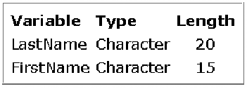
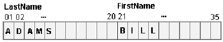
In uncompressed form,
each observation in Roster uses a total of 35 bytes to store these
two variables: 20 bytes for the first variable, LastName, and 15 bytes
for the second variable, FirstName. The image below illustrates the
storage of the first observation in the uncompressed version of Roster.
Suppose that you use
the CHAR setting for the COMPRESS= option to compress Roster. In compressed
form, the repeated blanks are removed from each value. The first observation
from Roster uses a total of only 13 bytes: 7 for the first variable,
LastName, and 6 for the second variable, FirstName. The image below
illustrates the storage of the first observation in the compressed
version of Roster.
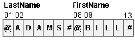
The @ indicates the
number of uncompressed characters that follow. The # indicates the
number of blanks that are repeated at this point in the observation.
Only a SAS engine can access these bytes. You cannot print or manipulate
them.
Ross Data Compression
(COMPRESS=BINARY) uses both run-length encoding and sliding window
compression. Suppose a SAS data set has these variables:
In uncompressed form,
the SAS data file resembles this:
1     2     3     4     5     6     7     8     9
@     +/1   1     #     @    +/1    2     #     %
The @ symbol indicates
how many uncompressed characters follow. In the file, +/1 is the
sign and exponent. The # indicates the number of binary zeros that
were removed. The % represents how many times these values are repeated.
Note: Remember that in a compressed
data set, observations might not all have the same length because
the length of an observation depends on the length of each value in
the observation.
Comparative Example: Creating and Reading Compressed Data Files
Overview
Suppose you want to
create two SAS data sets from data that is stored in two raw data
files. The raw data file that is referenced by the fileref Flat1 contains
numeric data about customer orders for a retail company; you want
to create a SAS data set named Retail.Orders from this raw data file.
The raw data file that is referenced by the fileref Flat2 contains
character data about customers for a retail company; you want to create
a SAS data set named Retail.Customers from this raw data file.
In both cases, you can
use the DATA step to create either an uncompressed data file or a
compressed data file. Furthermore, you can use either binary or character
compression in either case.
The following sample
programs compare six techniques. You can use these samples as models
for creating benchmark programs in your own environment. Your results
might vary depending on the structure of your data, your operating
environment, and the resources that are available at your site.
Programming Techniques
|
The following program
creates the SAS data set Retail.Orders, which contains numeric data
and is uncompressed. The second DATA step reads the uncompressed data
file.
data retail.orders(compress=no);
   infile flat1;
   input  Customer_ID          12.
          Employee_ID          12.
          Street_ID            12.
          Order_Date           date9.
          Delivery_Date        date9.
          Order_ID             12.
          Order_Type           comma16.
          Product_ID           12.
          Quantity             4.
          Total_Retail_Price   dollar13.
          CostPrice_Per_Unit   dollar13.
          Discount             5.            ;
run;

data _null_;
   set retail.orders;
run; |
|
The following program
creates the SAS data set Retail.Orders_binary, which contains numeric
data and uses BINARY compression. The second DATA step reads the compressed
data file.
data retail.orders_binary(compress=binary);
   infile flat1;
   input  Customer_ID          12.
          Employee_ID          12.
          Street_ID            12.
          Order_Date           date9.
          Delivery_Date        date9.
          Order_ID             12.
          Order_Type           comma16.
          Product_ID           12.
          Quantity             4.
          Total_Retail_Price   dollar13.
          CostPrice_Per_Unit   dollar13.
          Discount             5.       ;
run;

data _null_;
   set retail.orders_binary;
run; |
|
The following program
creates the SAS data set Retail.Orders_char, which contains numeric
data and uses CHAR compression. The second DATA step reads the compressed
data file.
data retail.orders_char(compress=char);
   infile flat1;
   input  Customer_ID          12.
          Employee_ID          12.
          Street_ID            12.
          Order_Date           date9.
          Delivery_Date        date9.
          Order_ID             12.
          Order_Type           comma16.
          Product_ID           12.
          Quantity             4.
          Total_Retail_Price   dollar13.
          CostPrice_Per_Unit   dollar13.
          Discount             5.       ;
run;

data _null_;
   set retail.orders_char;
run; |
|
The following program
creates the SAS data set Retail.Customers, which contains character
data and is uncompressed. The second DATA step reads the uncompressed
data file.
data retail.customers(compress=no);
   infile flat2;
   input  Customer_Country     $40.
          Customer_Gender      $1.
          Customer_Name        $40.
          Customer_FirstName   $20.
          Customer_LastName    $30.
          Customer_Age_Group   $12.
          Customer_Type        $40.
          Customer_Group       $40.
          Customer_Address     $45.
          Street_Number        $8.           ;
run;

data _null_;
   set retail.cutomers;
run; |
|
The following program
creates the SAS data set Retail.Customers_binary, which contains character
data and uses BINARY compression. The second DATA step reads the compressed
data file.
data retail.customers_binary(compress=binary);
   infile flat2;
   input  Customer_Country     $40.
          Customer_Gender      $1.
          Customer_Name        $40.
          Customer_FirstName   $20.
          Customer_LastName    $30.
          Customer_Age_Group   $12.
          Customer_Type        $40.
          Customer_Group       $40.
          Customer_Address     $45.
          Street_Number        $8.           ;
run;

data _null_;
   set retail.customers_binary;
run; |
|
The following program
creates the SAS data set Retail.Customers_char, which contains character
data and uses CHAR compression. The second DATA step reads the compressed
data file.
data retail.customers_char(compress=char);
   infile flat2;
   input  Customer_Country     $40.
          Customer_Gender      $1.
          Customer_Name        $40.
          Customer_FirstName   $20.
          Customer_LastName    $30.
          Customer_Age_Group   $12.
          Customer_Type        $40.
          Customer_Group       $40.
          Customer_Address     $45.
          Street_Number        $8.           ;
run;

data _null_;
   set retail.customers_char;
run; |
..................Content has been hidden....................
You can't read the all page of ebook, please click here login for view all page.