
Chapter 12. A picture is worth 1024 words
The Chemical Tracking System (CTS) project team was holding its first detailed requirements review. The participants were Dave (project manager), Lori (business analyst), Helen (lead developer), Ramesh (test lead), Tim (product champion for the chemists), and Roxanne (product champion for the chemical stockroom staff). Tim began by saying, “I read the whole document. Most of the requirements seemed okay to me, but I had a hard time digesting the long lists of requirements in a few sections. I’m not sure whether we identified all the steps in the chemical request process.”
“It was hard for me to think of all the tests that I’ll need to cover the status changes for a request,” Ramesh added. “I found a bunch of requirements sprinkled throughout the document about the status changes, but I couldn’t tell whether any were missing. A couple of requirements seemed to conflict.”
Roxanne had a similar problem. “I got confused when I read about the way I would actually request a chemical,” she said. “I had trouble visualizing the sequence of steps I would go through.”
After the reviewers raised several other concerns, Lori concluded, “It looks like this document doesn’t tell us everything we need to know about the system. I’ll create some diagrams to help us visualize the requirements and see whether that clarifies these problem areas. Thanks for the feedback.”
As requirements authority Alan Davis pointed out, no single view of the requirements provides a complete understanding ([ref055]). You need a combination of textual and visual requirements representations at different levels of abstraction to paint a full picture of the intended system. Requirements views can include functional requirements lists, tables, visual analysis models, user interface prototypes, acceptance tests, decision trees, decision tables, photographs, videos, and mathematical expressions ([ref247]). Ideally, different people will create various requirements representations. The business analyst might write the functional requirements and draw some models, whereas the user interface designer builds a prototype and the test lead writes test cases. Comparing the requirements representations created through diverse thought processes and diverse notations reveals inconsistencies, ambiguities, assumptions, and omissions that are difficult to spot from any single view.
Diagrams communicate certain types of information more efficiently than text can. Pictures help bridge language and vocabulary barriers among team members. The BA initially might need to explain the purpose of the models and the notations used to other stakeholders. There are many different diagrams and modeling techniques to choose from to create visual representations of the requirements. This chapter introduces several requirements modeling techniques, with illustrations and pointers to other sources for further details.
Modeling the requirements
Business analysts might hope to find one technique that pulls everything together into a holistic depiction of a system’s requirements. Unfortunately, there is no such all-encompassing diagram. In fact, if you could model the entire system in a single diagram, that diagram would be just as unusable as a long list of requirements on its own. An early goal of structured systems analysis was to replace the classical functional specification with diagrams and notations that are more formal than narrative text. However, experience has shown that analysis models should augment—rather than replace—a requirements specification written in natural language. Developers and testers still benefit from the detail and precision that written requirements offer.
Visual requirements models can help you identify missing, extraneous, and inconsistent requirements. Given the limitations of human short-term memory, analyzing a list of one thousand requirements for inconsistencies, duplication, and extraneous requirements is nearly impossible. By the time you reach the fifteenth requirement, you have likely forgotten the first few that you read. You’re unlikely to find all of the errors simply by reviewing the textual requirements.
Visual requirements models described in this book include:
Data flow diagrams (DFDs)
Process flow diagrams such as swimlane diagrams
State-transition diagrams (STDs) and state tables
Dialog maps
Decision tables and decision trees
Event-response tables
Feature trees (discussed in Chapter 5)
Use case diagrams (discussed in Chapter 8)
Activity diagrams (also discussed in Chapter 8)
Entity-relationship diagrams (ERDs) (discussed in Chapter 13)
The notations presented here provide a common, industry-standard language for project participants to use. Inventing your own modeling notations presents more risk of misinterpretation than if you adopt standard notations.
These models are useful for elaborating and exploring the requirements, as well as for designing software solutions. Whether you are using them for analysis or for design depends on the timing and the intent of the modeling. Used for requirements analysis, these diagrams let you model the problem domain or create conceptual representations of the new system. They depict the logical aspects of the problem domain’s data components, transactions and transformations, real-world objects, and changes in system state. You can base the models on the textual requirements to represent them from different perspectives, or you can derive functional requirements from high-level models that are based on user input. During design, models represent how you intend to implement the system: the actual database to create, the object classes to instantiate, and the code modules to develop. Because analysis and design diagrams use the same notations, clearly identify each one you draw as being an analysis model (the concepts) or a design model (what you intend to build).
The analysis modeling techniques described in this chapter are supported by a variety of commercial modeling tools, requirements management tools, and drawing tools such as Microsoft Visio. Specialized modeling tools provide several benefits over general-purpose drawing tools. First, they make it easy to improve the diagrams through iteration. You’ll almost never get a model right the first time through, so iteration is a key to modeling success. Tools can also enforce the rules for each modeling method they support. They can identify syntax errors and inconsistencies that people who review the diagrams might not see. Requirements management tools that support modeling allow you to trace requirements to the models. Some tools link multiple diagrams together and to their related functional and data requirements. Using a tool with standard symbols can help you keep the models consistent with each other.
We hear arguments against using requirements models that range from “Our system is too complex to model” to “We have a tight project schedule; there is no time to model the requirements.” A model is simpler than the system you are modeling. If you cannot handle the complexity of the model, how will you be able to handle the complexity of the system? Creating most models doesn’t require significantly more time than you would spend writing the requirements statements and analyzing them for issues. Any extra time spent using requirements analysis models should be more than made up for by catching requirements errors prior to building the system. Models, or portions of models, can sometimes be reused from one project to another, or at least serve as a straw-man starting point for requirements elicitation on a subsequent project.
From voice of the customer to analysis models
By listening carefully to how customers present their requirements, the business analyst can pick out keywords that translate into specific model elements. Table 12-1 suggests possible mappings from customers’ word choices into model components, which are described later in this chapter. As you evolve customer input into written requirements and models, you should be able to link each model component to a specific user requirement.
Type of word | Examples | Analysis model components |
Noun | People, organizations, software systems, data elements, or objects that exist |
|
Verb | Actions, things a user or system can do, or events that can take place |
|
Conditional | Conditional logic statements, such as if/then |
|
Building on the Chemical Tracking System example, consider the following paragraph of user needs supplied by the product champion who represented the Chemist user class. Significant unique nouns are highlighted in bold, verbs are in italics, and conditional statements are in bold italics; look for these keywords in the analysis models shown later in this chapter. For the sake of illustration, some of the models show information that goes beyond that contained in the following paragraph, whereas other models depict just part of the information presented here:
A chemist or a member of the chemical stockroom staff can place a request for one or more chemicals if the user is an authorized requester. The request can be fulfilled either by delivering a container of the chemical that is already in the chemical stockroom’s inventory or by placing an order for a new container of the chemical with an outside vendor. If the chemical is hazardous, the chemical can be delivered only if the user is trained. The person placing the request must be able to search vendor catalogs online for specific chemicals while preparing his request. The system needs to track the status of every chemical request from the time it is prepared until the request is either fulfilled or canceled. It also needs to track the history of every chemical container from the time it is received at the company until it is fully consumed or disposed of.
Trap
Don’t assume that customers already know how to read analysis models, but don’t conclude that they’re unable to understand them, either. Include a key and explain the purpose and notations of each model to your product champions. Walk through a sample model to help them learn how to review each type of diagram.
Selecting the right representations
Rarely does a team need to create a complete set of analysis models for an entire system. Focus your modeling on the most complex and riskiest portions of the system and on those portions most subject to ambiguity or uncertainty. Safety-critical, security-critical, and mission-critical system elements are good candidates for modeling because the impact of defects in those areas is so severe. Also choose models to use together to help ensure all of the models are complete. For example, examining the data objects in a DFD can uncover missing entities in an ERD. Considering all the processes in a DFD might identify useful swimlane diagrams to create. There are suggestions throughout the rest of the chapter on which models complement each other well in this fashion.
Table 12-2, adapted from Karl Wiegers’ work (2006), suggests which representation techniques to use based on what type of information you are trying to show, analyze, or discover. [ref013] provide additional suggestions about what requirements models to create based on project phases, characteristics of the project, and the target audience(s) for the models. The rest of this chapter describes some of the most commonly used models from this table that are not covered elsewhere in the book.
Information depicted | Representation techniques |
System external interfaces |
|
Business process flow |
|
Data definitions and data object relationships |
|
| |
Complex logic |
|
User interfaces |
|
User task descriptions |
|
Nonfunctional requirements (quality attributes, constraints) |
|
Data flow diagram
The data flow diagram is the basic tool of structured analysis ([ref059]; [ref200]). A DFD identifies the transformational processes of a system, the collections (stores) of data or physical materials that the system manipulates, and the flows of data or material between processes, stores, and the outside world. Data flow modeling takes a functional decomposition approach to systems analysis, breaking complex problems into progressive levels of detail. This works well for transaction-processing systems and other function-intensive applications. Through the addition of control flow elements, the DFD technique has been extended to permit modeling of real-time systems ([ref106]).
DFDs provide a big-picture view of how data moves through a system, which other models don’t show well. Various people and systems execute processes that use, manipulate, and produce data, so any single use case or swimlane diagram can’t show you the full life cycle of a piece of data. Also, multiple pieces of data might be pulled together and transformed by a process (for example, shopping cart contents plus shipping information plus billing information are transformed into an order object). Again, this is hard to show in other models. However, DFDs do not suffice as a sole modeling technique. The details about how the data is transformed are better shown by steps in a process using use cases or swimlane diagrams.
[ref013] suggest tips for creating DFDs and using DFDs for requirements analysis. This tool is often used when interviewing customers, because it’s easy to scribble a DFD on a whiteboard while discussing how the user’s business operates. DFDs can be used as a technique to identify missing data requirements. The data that flows between processes, data stores, and external entities should also be modeled in ERDs and described in the data dictionary. Also, a DFD gives context to the functional requirements regarding how the user performs specific tasks, such as requesting a chemical.
Data flow diagrams can represent systems over a wide range of abstraction. High-level DFDs provide a holistic, bird’s-eye view of the data and processing components in a multistep activity, which complements the precise, detailed view embodied in the functional requirements. The context diagram in Figure 5-6 in Chapter 5 represents the highest level of abstraction of the DFD. The context diagram represents the entire system as a single black-box process, depicted as a circle (a bubble). It also shows the external entities, or terminators, that connect to the system, and the data or material flows between the system and the external entities. Flows on a context diagram often represent complex data structures, which are defined in the data dictionary.
You can elaborate the context diagram into a level 0 DFD (the highest level of a data flow model), which partitions the system into its major processes. Figure 12-1 shows a partial level 0 DFD for the Chemical Tracking System. This model uses the Yourdon-DeMarco DFD notation. There are alternative notations that use slightly different symbols.
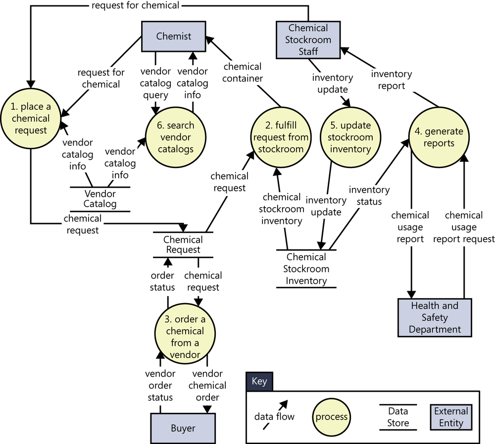
The single circle that represented the entire Chemical Tracking System on the context diagram has been subdivided into six major processes (the process bubbles). As with the context diagram, the external entities are shown in rectangles. All data flows (arrows) from the context diagram also appear on the level 0 DFD. In addition, the level 0 diagram contains several data stores, depicted as a pair of parallel horizontal lines, which are internal to the system and therefore do not appear on the context diagram. A flow from a bubble to a store indicates that data is being placed into the store, a flow out of the store shows a read operation, and a bidirectional arrow between a store and a bubble indicates an update operation.
Each process that appears as a separate bubble on the level 0 diagram can be further expanded into a separate DFD to reveal more detail about its functioning. The BA continues this progressive refinement until the lowest-level diagrams contain only primitive process operations that can be clearly represented in narrative text, pseudocode, a swimlane diagram, or an activity diagram. The functional requirements will define precisely what happens within each primitive process. Each level of the DFD must be balanced and consistent with the level above it so that all the input and output flows on the child diagram match up with flows on its parent. Complex data structures in the high-level diagrams might be split into their constituent elements, as defined in the data dictionary, on the lower-level DFDs.
Figure 12-1 looks complex at first glance. However, if you examine the immediate environment of any one process, you will see the data items that it consumes and produces and their sources and destinations. To see exactly how a process uses the data items, you’ll need to either draw a more detailed child DFD or refer to the functional requirements for that part of the system.
Following are several conventions for drawing data flow diagrams. Not everyone adheres to the same conventions (for example, some BAs show external entities only on the context diagram), but we find them helpful. Using the models to enhance communication among the project participants is more important than dogmatic conformance to these principles.
Processes communicate through data stores, not by direct flows from one process to another. Similarly, data cannot flow directly from one store to another or directly between external entities and data stores; it must pass through a process bubble.
Don’t attempt to imply the processing sequence using the DFD.
Name each process as a concise action: verb plus object (such as “generate reports”). Use names that are meaningful to the customers and pertinent to the business or problem domain.
Number the processes uniquely and hierarchically. On the level 0 diagram, number each process with an integer. If you create a child DFD for process 3, number the processes in that child diagram 3.1, 3.2, and so on.
Don’t show more than 8 to 10 processes on a single diagram or it will be difficult to draw, change, and understand. If you have more processes, introduce another layer of abstraction by grouping related processes into a higher-level process.
Bubbles with flows that are only coming in or only going out are suspect. The processing that a DFD bubble represents normally requires both input and output flows.
When customer representatives review a DFD, they should make sure that all the known and relevant data-manipulating processes are represented and that processes have no missing or unnecessary inputs or outputs. DFD reviews often reveal previously unrecognized user classes, business processes, and connections to other systems.
Swimlane diagram
Swimlane diagrams provide a way to represent the steps involved in a business process or the operations of a proposed software system. They are a variation of flowcharts, subdivided into visual subcomponents called lanes. The lanes can represent different systems or actors that execute the steps in the process. Swimlane diagrams are most commonly used to show business processes, workflows, or system and user interactions. They are similar to UML activity diagrams. Swimlane diagrams are sometimes called cross-functional diagrams.
Swimlane diagrams can show what happens inside the process bubbles from DFDs. They help tie together the functional requirements that enable users to perform specific tasks. They can also be used to perform detailed analysis to identify the requirements that support each process step ([ref013]).
The swimlane diagram is one of the easiest models for stakeholders to understand because the notation is simple and commonly used. Drafting business processes in swimlane diagrams can be a good starting point for elicitation conversations, as is described in Chapter 24. Swimlane diagrams can contain additional shapes, but the most commonly used elements are:
Process steps, shown as rectangles.
Transitions between process steps, shown as arrows connecting pairs of rectangles.
Decisions, shown as diamonds with multiple branches leaving each diamond. The decision choices are shown as text labels on each arrow leaving a diamond.
Swimlanes to subdivide the process, shown as horizontal or vertical lines on the page. The lanes are most commonly roles, departments, or systems. They show who or what is executing the steps in a given lane.
Figure 12-2 shows a partial swimlane diagram for the CTS. The swimlanes in this example are roles or departments, showing which group executes each step in the business process to order a chemical from a vendor. To identify functional requirements, you can start at the first box, “Create a chemical request,” and think about what functionality the system must have to support that step, as well as the data requirements for a “chemical request.” A later step to “Receive and approve invoice” might trigger the team to identify requirements for what it means to process an invoice. How is the invoice received? What is its format? Is the invoice processing manual, or does the system automate some or all of it? Does the data from the invoice get pushed to other systems?
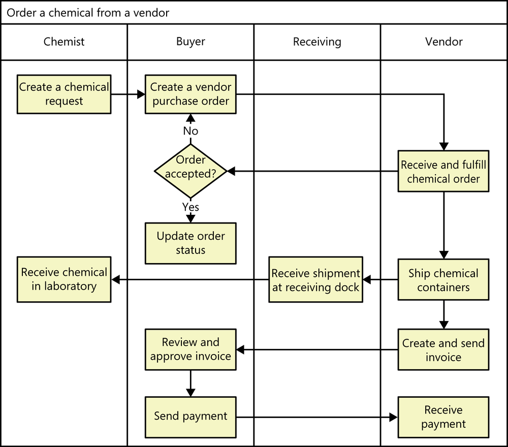
A complete business process might not fit entirely within the scope of a software system. Notice that the Receiving department appears in the swimlane as part of the process, but it is not found in the context diagram or the DFD because the Receiving department will never interact with the CTS directly. Reviewing the ecosystem map shown in Figure 5-7 (shown earlier, in Chapter 5) triggered the team to realize that Receiving had a place in this business process, though. The team also reviewed the data inputs to and outputs from this process bubble in the DFD (process 3 in Figure 12-1) to ensure that both models consumed and produced the same data, correcting any errors they found. This illustrates the power of modeling, creating multiple representations using different thought processes to gain a richer understanding of the system you’re building.
State-transition diagram and state table
Software systems involve a combination of functional behavior, data manipulation, and state changes. Real-time systems and process control applications can exist in one of a limited number of states at any given time. A state change can take place only when well-defined criteria are satisfied, such as receiving a specific input stimulus under certain conditions. An example is a highway intersection that incorporates vehicle sensors, protected turn lanes, and pedestrian crosswalk buttons and signals. Many information systems deal with business objects—sales orders, invoices, inventory items, and the like—with life cycles that involve a series of possible states, or statuses.
Describing a set of complex state changes in natural language creates a high probability of overlooking a permitted state change or including a disallowed change. Depending on how an SRS is organized, requirements that pertain to the state-driven behavior might be sprinkled throughout it. This makes it difficult to reach an overall understanding of the system’s behavior.
State-transition diagrams and state tables are two state models that provide a concise, complete, and unambiguous representation of the states of an object or system. The state-transition diagram (STD) shows the possible transitions between states visually. A related technique is the state machine diagram included in the Unified Modeling Language (UML), which has a richer set of notations and which models the states an object goes through during its lifetime ([ref006]). The STD contains three types of elements:
Possible system states, shown as rectangles. Some notations use circles to represent the state ([ref013]). Either circles or rectangles work fine; just be consistent in what you choose to use.
Allowed state changes or transitions, shown as arrows connecting pairs of rectangles.
Events or conditions that cause each transition to take place, shown as text labels on each transition arrow. The label might identify both the event and the corresponding system response.
The STD for an object that passes through a defined life cycle will have one or more termination states, which represent the final status values that an object can have. Termination states have transition arrows coming in, but none going out. Customers can learn to read an STD with just a little coaching about the notation—it’s just boxes and arrows.
Recall from Chapter 8 that a primary function of the Chemical Tracking System is to permit actors called Requesters to place requests for chemicals, which can be fulfilled either from the chemical stockroom’s inventory or by placing orders to outside vendors. Each request will pass through a series of states between the time it’s created and the time it’s either fulfilled or canceled (the two termination states). Thus, an STD models the life cycle of a chemical request, as shown in Figure 12-3.
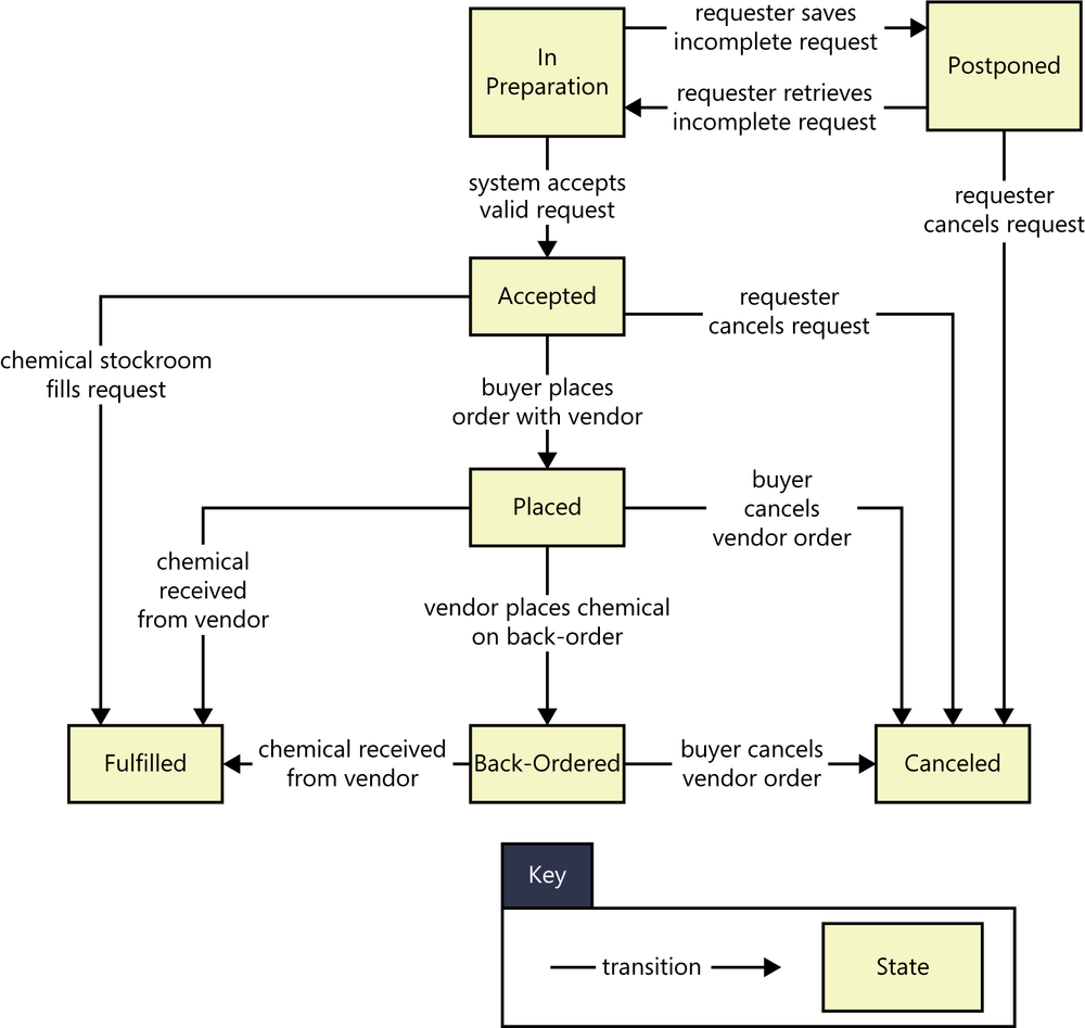
This STD shows that an individual request can take on one of the following seven possible states:
In Preparation. The Requester is creating a new request, having initiated that function from some other part of the system.
Postponed. The Requester saved a partial request for future completion without either submitting the request to the system or canceling the request operation.
Accepted. The Requester submitted a completed chemical request and the system accepted it for processing.
Placed. The request must be satisfied by an outside vendor and a buyer has placed an order with the vendor.
Fulfilled. The request has been satisfied, either by the delivery of a chemical container from the chemical stockroom to the Requester or by receipt of a chemical from a vendor.
Back-ordered. The vendor didn’t have the chemical available and notified the buyer that it was back-ordered for future delivery.
Canceled. The Requester canceled an accepted request before it was fulfilled, or the buyer canceled a vendor order before it was fulfilled or while it was back-ordered.
When the Chemical Tracking System user representatives reviewed the initial chemical request STD, they identified one state that wasn’t needed, saw that another essential state was missing, and pointed out two incorrect transitions. No one had seen those errors when they reviewed the corresponding functional requirements. This underscores the value of representing requirements information at more than one level of abstraction. It’s often easier to spot a problem when you step back from the detailed level and see the big picture that an analysis model provides. However, the STD doesn’t provide enough detail for a developer to know what software to build. Therefore, the SRS for the Chemical Tracking System included the functional requirements associated with processing a chemical request and its possible state changes.
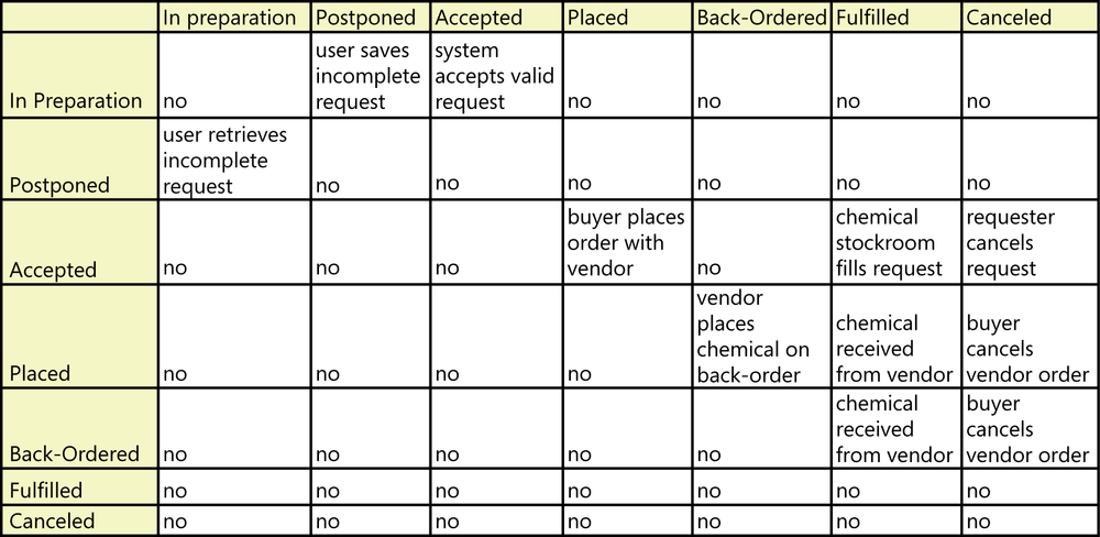
A state table shows all of the possible transitions between states in the form of a matrix. A business analyst can use state tables to ensure that all transitions are identified by analyzing every cell in the matrix. All states are written down the first column and repeated across the first row of the table. The cells indicate whether the transition from a state on the left to a state at the top is valid, and identifies the transition event to move between states. Figure 12-4 shows a state table that matches the state-transition diagram in Figure 12-3. These two diagrams show exactly the same information, but the table format helps ensure that no transitions are missed, and the diagram format helps stakeholders visualize the possible sequences of transitions. You might not need to create both models. However, if you have created one already, the other is easy to create, if you do want to analyze the state changes from two perspectives. The two rows in Figure 12-4 in which the values are all “no” are both termination states; when the chemical request is in either the Fulfilled or the Canceled state, it cannot transition out of it.
The state-transition diagram and state table provide a high-level viewpoint that spans multiple use cases or user stories, each of which might perform a transition from one state to another. The state models don’t show the details of the processing that the system performs; they show only the possible state changes that result from that processing. They help developers understand the intended behavior of the system. The models facilitate early testing because testers can derive tests from the STD that cover all allowed transition paths. Both models are useful for ensuring that all the required states and transitions have been correctly and completely described in the functional requirements.
Dialog map
The dialog map represents a user interface design at a high level of abstraction. It shows the dialog elements in the system and the navigation links among them, but it doesn’t show the detailed screen designs. A user interface can be regarded as a series of state changes. Only one dialog element (such as a menu, workspace, dialog box, line prompt, or touch screen display) is available at any given time for user input. The user can navigate to certain other dialog elements based on the action he takes at the active input location. The number of possible navigation pathways can be large in a complex system, but the number is finite and the options are usually known. A dialog map is really just a user interface modeled in the form of a state-transition diagram ([ref238]; [ref240]). [ref049] describe a similar technique called a navigation map, which includes a richer set of notations for representing different types of interaction elements and context transitions. A user interface flow is similar to a dialog map but shows the navigation paths between user interface screens in a swimlane diagram format ([ref013]).
A dialog map allows you to explore hypothetical user interface concepts based on your understanding of the requirements. Users and developers can study a dialog map to reach a common vision of how the user might interact with the system to perform a task. Dialog maps are also useful for modeling the visual architecture of a website. Navigation links that you build into the website appear as transitions on the dialog map. Of course, the user has additional navigation options through the browser’s Back and Forward buttons, as well as the URL input field, but the dialog map does not show those. Dialog maps are related to system storyboards, which also include a short description of each screen’s purpose ([ref158]).
Dialog maps capture the essence of the user–system interactions and task flow without bogging the team down in detailed screen layouts. Users can trace through a dialog map to find missing, incorrect, or unnecessary navigations, and hence missing, incorrect, or unnecessary requirements. The abstract, conceptual dialog map formulated during requirements analysis serves as a guide during detailed user interface design.
Just as in ordinary state-transition diagrams, the dialog map shows each dialog element as a state (rectangle) and each allowed navigation option as a transition (arrow). The condition that triggers user interface navigation is shown as a text label on the transition arrow. There are several types of trigger conditions:
A user action, such as pressing a function key, clicking on a hyperlink, or making a gesture on a touch screen.
A data value, such as an invalid user input value that triggers an error message display
A system condition, such as detecting that a printer is out of paper
Some combination of these, such as typing a menu option number and pressing the Enter key
Dialog maps look a bit like flowcharts, but they serve a different purpose. A flowchart explicitly shows the processing steps and decision points, but not the user interface displays. In contrast, the dialog map does not show the processing that takes place along the transition lines that connect one dialog element to another. The branching decisions (usually user choices) are hidden behind the display screens that are shown as rectangles on the dialog map, and the conditions that lead to displaying one screen or another appear in the labels on the transitions.
To simplify the dialog map, omit global functions such as pressing the F1 key to bring up a help display from each dialog element. The SRS section on user interfaces should specify that this functionality will be available, but showing lots of help-screen boxes on the dialog map clutters the model while adding little value. Similarly, when modeling a website, you needn’t include standard navigation links that will appear on each page in the site. You can also omit the transitions that reverse the flow of a webpage navigation sequence because the web browser’s Back button handles that navigation.
A dialog map is an excellent way to represent the interactions between an actor and the system that a use case describes. The dialog map can depict alternative flows as branches off the normal flow. I found that sketching dialog map fragments on a whiteboard was helpful during use case elicitation workshops in which a team explored the sequence of actor actions and system responses that would lead to task completion. For use cases and process flows that are already complete, compare them to dialog maps to ensure that all the functions needed to execute the steps can be accessed in the UI navigation.
Chapter 8 presented a use case for the Chemical Tracking System called “Request a Chemical.” The normal flow for this use case involved requesting a chemical container from the chemical stockroom’s inventory. An alternative flow was to request the chemical from a vendor. The user placing the request wanted the option to view the history of the available stockroom containers of that chemical before selecting one. Figure 12-5 shows a dialog map for this fairly complex use case. The entry point for this dialog map is the transition line that begins with a solid black circle, “ask to place a request.” The user would enter this portion of the application’s user interface from some other part of the UI along that line. Exit points for the dialog map to return to some other portion of the UI are the transition lines ending with a solid black circle inside another circle, “cancel entire request” and “OK; exit request function.”
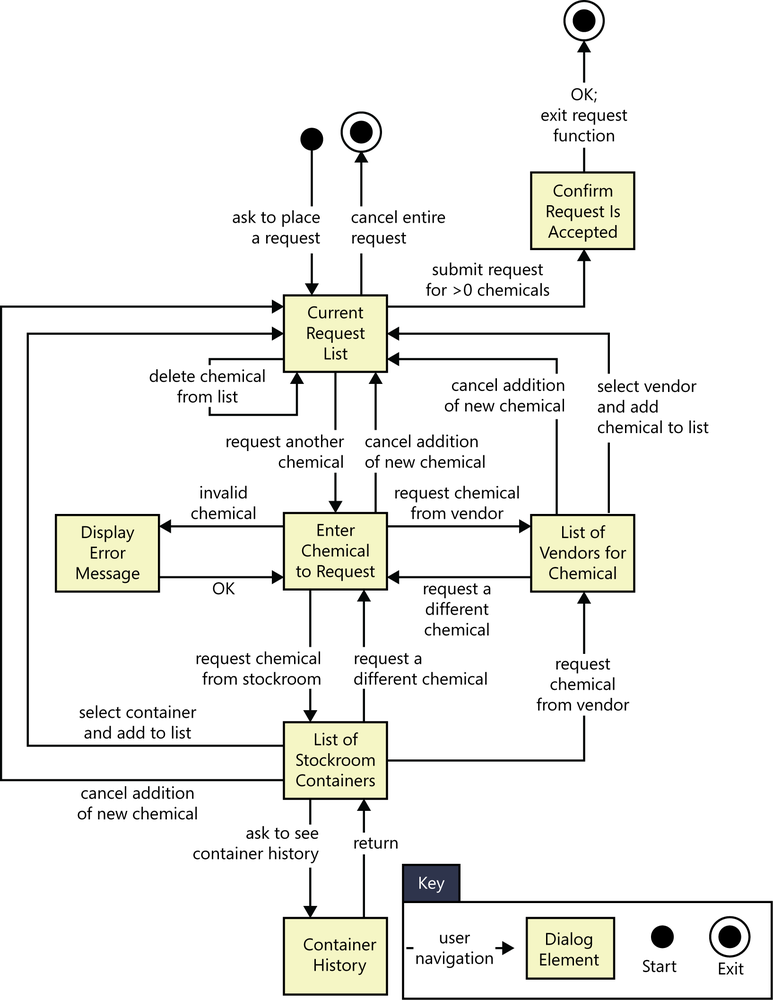
This diagram might look complicated at first, but if you trace through it one line and one box at a time, it’s not difficult to understand. The user initiates this use case by asking to place a request for a chemical from some menu in the Chemical Tracking System. In the dialog map, this action brings the user to the box called “Current Request List,” along the arrow in the upper-left part of the dialog map. That box represents the main workspace for this use case, a list of the chemicals in the user’s current request. The arrows leaving that box on the dialog map show all the navigation options—and hence functionality—available to the user in that context:
Cancel the entire request.
Submit the request if it contains at least one chemical.
Add a new chemical to the request list.
Delete a chemical from the list.
The last operation, deleting a chemical, doesn’t involve another dialog element; it simply refreshes the current request list display after the user makes the change.
As you trace through this dialog map, you’ll see elements that reflect the rest of the “Request a Chemical” use case:
One flow path for requesting a chemical from a vendor
Another path for fulfillment from the chemical stockroom
An optional path to view the history of a container in the chemical stockroom
An error message display to handle entry of an invalid chemical identifier or other error conditions that could arise
Some of the transitions on the dialog map allow the user to back out of operations. Users get annoyed if they are forced to complete a task even though they change their minds partway through it. The dialog map lets you maximize usability by designing in those back-out and cancel options at strategic points.
A user who reviews this dialog map might spot a missing requirement. For example, a cautious user might want to confirm the operation that leads to canceling an entire request to avoid inadvertently losing data. It costs less to add this new function at the analysis stage than to build it into a completed product. Because the dialog map represents just the conceptual view of the possible elements involved in the interaction between the user and the system, don’t try to pin down all the user interface design details at the requirements stage. Instead, use these models to help the project stakeholders reach a common understanding of the system’s intended functionality.
Decision tables and decision trees
A software system is often governed by complex logic, with various combinations of conditions leading to different system behaviors. For example, if the driver presses the accelerate button on a car’s cruise control system and the car is currently cruising, the system increases the car’s speed, but if the car isn’t cruising, the input is ignored. Developers need functional requirements that describe what the system should do under all possible combinations of conditions. However, it’s easy to overlook a condition, which results in a missing requirement. These gaps are hard to spot by reviewing a textual specification.
Decision tables and decision trees are two alternative techniques for representing what the system should do when complex logic and decisions come into play ([ref013]). A decision table lists the various values for all the factors that influence the behavior and indicates the expected system action in response to each combination of factors. The factors can be shown either as statements with possible conditions of true and false, as questions with possible answers of yes and no, or as questions with more than two possible values.
Figure 12-6 shows a decision table for the logic that governs whether the Chemical Tracking System should accept or reject each request for a new chemical. Four factors influence this decision:
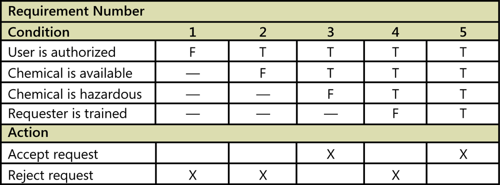
Whether the user who is creating the request is authorized to request chemicals
Whether the chemical is available either in the chemical stockroom or from a vendor
Whether the chemical is on the list of hazardous chemicals that require special training in safe handling
Whether the user who is creating the request has been trained in handling this type of hazardous chemical
Each of these four factors has two possible conditions, true or false. In principle, this gives rise to 24, or 16, possible true/false combinations, for a potential of 16 distinct functional requirements. In practice, though, many of the combinations lead to the same system response. If the user isn’t authorized to request chemicals, then the system won’t accept the request, so the other conditions are irrelevant (shown as dashes in the cells in the decision table). The table shows that only five distinct functional requirements arise from the various combinations.
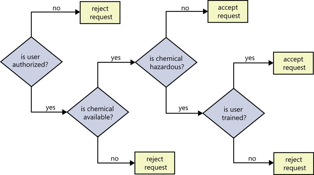
Figure 12-7 shows a decision tree that represents this same logic. The five boxes indicate the five possible outcomes of either accepting or rejecting the chemical request. Both decision tables and decision trees are useful ways to document requirements (or business rules) to avoid overlooking any combinations of conditions. Even a complex decision table or tree is easier to read than a mass of repetitious textual requirements.
Event-response tables
Use cases and user stories aren’t always helpful or sufficient for discovering the functionality that developers must implement ([ref247]). This is particularly true for real-time systems. Consider a complex highway intersection with numerous traffic lights and pedestrian walk signals. There aren’t many use cases for a system like this. A driver might want to proceed through the light or to turn left or right. A pedestrian wants to cross the road. Perhaps an emergency vehicle wants to be able to turn the traffic signals green in its direction so it can speed its way to people who need help. Law enforcement might have cameras at the intersection to photograph the license plates of red-light violators. This information alone isn’t enough for developers to build the correct functionality.
Another way to approach user requirements is to identify the external events to which the system must respond. An event is some change or activity that takes place in the user’s environment that stimulates a response from the software system ([ref250]). An event-response table (also called an event table or an event list) itemizes all such events and the behavior the system is expected to exhibit in reaction to each event. There are three classes of system events, as shown in Figure 12-8:
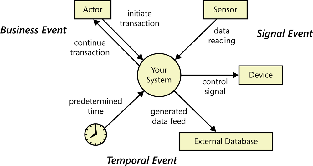
Business event. A business event is an action by a human user that stimulates a dialog with the software, as when the user initiates a use case. The event-response sequences correspond to the steps in a use case or swimlane diagram.
Signal event. A signal event is registered when the system receives a control signal, data reading, or interrupt from an external hardware device or another software system, such as when a switch closes, a voltage changes, another application requests a service, or a user swipes his finger on a tablet’s screen.
Temporal event. A temporal event is time-triggered, as when the computer’s clock reaches a specified time (say, to launch an automatic data export operation at midnight) or when a preset duration has passed since a previous event (as in a system that logs the temperature read by a sensor every 10 seconds).
Event analysis works especially well for specifying real-time control systems. To identify events, consider all the states associated with the object you are analyzing, and identify any events that might transition the object into those states. Review context diagrams for any external entities that might initiate an action (trigger an event) or require an automatic response (need a temporal event triggered). Table 12-3 contains a sample event-response table that partially describes the behavior of an automobile’s windshield wipers. Other than event 6, which is a temporal event, these are all signal events. Note that the expected response depends not only on the event but also on the state of the system at the time the event takes place. For instance, events 4 and 5 in Table 12-3 result in slightly different behaviors depending on whether the wipers were on at the time the user set the wiper control to the intermittent setting. A response could simply alter some internal system information or it could result in an externally visible result. Other information you might want to add to an event-response table includes:
ID | Event | System state | System response |
1 | Set wiper control to low speed | Wiper off, on high speed, or on intermittent | Set wiper motor to low speed |
2 | Set wiper control to high speed | Wiper off, on low speed, or on intermittent | Set wiper motor to high speed |
3 | Set wiper control to off | Wiper on high speed, low speed, or intermittent |
|
4 | Set wiper control to intermittent | Wiper off |
|
5 | Set wiper control to intermittent | Wiper on low speed or on high speed |
|
6 | Wipe time interval has passed since completing last cycle | Wiper on intermittent | Perform one wipe cycle at low speed setting |
7 | Change intermittent wiper interval | Wiper on intermittent |
|
8 | Change intermittent wiper interval | Wiper off, on high speed, or on low speed | No response |
9 | Immediate wipe signal received | Wiper off | Perform one low-speed wipe cycle |
The event frequency (how many times the event takes place in a given time period, or a limit to how many times it can occur).
Data elements that are needed to process the event.
The state of the system after the event responses are executed ([ref094]).
Listing the events that cross the system boundary is a useful scoping technique ([ref247]). An event-response table that defines every possible combination of event, state, and response, including exception conditions, can serve as part of the functional requirements for that portion of the system. You might model the event-response table in a decision table to ensure that all possible combinations of events and system states are analyzed. However, the BA must supply additional functional and nonfunctional requirements. How many cycles per minute does the wiper perform on the slow and fast wipe settings? Is the intermittent setting continuously variable, or does it have discrete settings? What are the minimum and maximum delay times between intermittent wipes? If you omit this sort of information, the developer has to track it down or make the decisions himself. Remember, the goal is to specify the requirements precisely enough that a developer knows what to build and a tester can determine if it was built correctly.
Notice that the events listed in Table 12-3 describe the essence of the event, not the specifics of the implementation. Table 12-3 shows nothing about how the windshield wiper controls look or how the user manipulates them. The designer could satisfy these requirements with anything from traditional stalk-mounted wiper controls to recognition of spoken commands: “wipers on,” “wipers faster,” “wipe once.” Writing requirements at the essential level like this avoids imposing unnecessary design constraints. However, record any known design constraints to guide the designer’s thinking.
A few words about UML diagrams
Many projects use object-oriented analysis, design, and development methods. Objects typically correspond to real-world items in the business or problem domain. They represent individual instances derived from a generic template called a class. Class descriptions encompass both attributes (data) and the operations that can be performed on the attributes. A class diagram is a graphical way to depict the classes identified during object-oriented analysis and the relationships among them (see Chapter 13).
Products developed using object-oriented methods don’t demand unique requirements development approaches. This is because requirements development focuses on what the users need to do with the system and the functionality it must contain, not with how it will be constructed. Users don’t care about objects or classes. However, if you know that you’re going to build the system using object-oriented techniques, it can be helpful to begin identifying classes and their attributes and behaviors during requirements analysis. This facilitates the transition from analysis to design, because the designer maps the problem-domain objects to the system’s objects and further details each class’s attributes and operations.
The standard object-oriented modeling language is the Unified Modeling Language ([ref025]). The UML is primarily used for creating design models. At the level of abstraction that’s appropriate for requirements analysis, several UML models can be useful ([ref076]; [ref188]):
Class diagrams, to show the object classes that pertain to the application domain; their attributes, behavior, and properties; and relations among classes. Class diagrams can also be used for data modeling, as illustrated in Chapter 13, but this limited application doesn’t fully exploit the semantic capabilities of a class diagram.
Use case diagrams, to show the relationships between actors external to the system and the use cases with which they interact (see Chapter 8).
Activity diagrams, to show how the various flows in a use case interlace, or which roles perform certain actions (as in a swimlane diagram), or to model the flow of business processes. See Chapter 8 for a simple example.
State (or state machine) diagrams, to represent the different states a system or data object can take on and the allowed transitions between the states.
Modeling on agile projects
All projects should exploit requirements models to analyze their requirements from a variety of perspectives, no matter what the project’s development approach is. The choice of models used across different development approaches will likely be the same. The difference in how traditional and agile projects perform modeling is related to when the models are created and the level of detail in them.
For example, you might draft a level 0 DFD early in an agile project. Then, during an iteration, you could draw more detailed DFDs to cover the scope of that iteration only. Also, you might create models in a less persistent or less perfected format on an agile project than on a traditional project. You might sketch an analysis model on a whiteboard and photograph it, but not store it with formal requirements documentation or in a modeling tool. As user stories are implemented, models can be updated (perhaps using color to indicate completeness), which shows what is being implemented in an iteration and reveals additional user stories that are needed to complete the picture.
The key point in using analysis models on agile projects—or really, on any project—is to focus on creating only the models you need, only when you need them, and only to the level of detail you need to make sure project stakeholders adequately understand the requirements. User stories won’t always be sufficient to capture the level of detail and precision necessary for an agile project ([ref157]). Do not rule out the use of any models just because you are working on an agile project.
A final reminder
Each of the modeling techniques described in this chapter has its strengths and its limitations. No one particular view will be sufficient to represent all aspects of the system. Also, they overlap in the views they provide, so you won’t need to create every kind of diagram for your project. For instance, if you create an ERD and a data dictionary, you probably won’t need to create a class diagram. Keep in mind that you draw analysis models to provide a level of understanding and communication that goes beyond what textual requirements or any other single view of the requirements can provide.