10 Infrared Measurements
The world Infrared Standard Group has been operating continuously since 2003, showing an excellent relative stability between individual instruments of ±1 W m–2.
Julian Gröbner
(2009)
10.1 Introduction
A body with a temperature above 0 K emits radiation. For the earth’s surface and atmospheric temperatures, this radiation is in the infrared (IR). The Stefan–Boltzmann law states that the power per unit area L emitted by a body of absolute temperature T is
In this equation σ is the Stefan–Boltzmann constant, equal to 5.670 x 10⁻⁸ W m–2 K–4, and ε is the emissivity of the body. If the emitting body is a gray body, then the emissivity is < 1; for a black body, ε is equal to 1. For example, if a pyrgeometer, which measures infrared radiation (see Section 10.2) is used to look at the surface of a parking lot, the temperature of the tarmac can be calculated very accurately, assuming an emissivity of 1. When looking at a clear sky, the temperature of the sky is more difficult to measure because there is no longer a near-perfect black body or gray body with a known emissivity. Figure 10.1 illustrates black-body spectral irradiance in power per unit area per unit wavelength at five temperatures: 250, 257, 275, 299 and 300 K. Looking at the two clear-sky curves in this figure, the spectral distribution of infrared radiation does not follow any of these curves at all wavelengths but does follow the 257 and 299 K black-body distributions at some of the wavelengths. So, what is going on in the sky? Parts of the infrared spectrum are completely absorbed by the molecules in the earth’s atmosphere; water vapor and carbon dioxide are especially significant absorbers. If there is little molecular absorption or there is only weak broadband extinction caused by aerosols, then the infrared spectrum will have “windows” that allow outgoing infrared radiation to escape. The “299 K Sky” plot in Figure 10.1 is for a modeled tropical clear sky. The “257 K Sky” plot in the same figure is for a modeled subarctic clear sky. Both tropical and subarctic clear skies exhibit significantly reduced irradiance at around 10 μm. This hole, or window if one is thinking of IR radiation from the earth passing through the atmosphere, is caused by the reduction in the number of molecules that emit, or absorb, radiation at these wavelengths, mainly, water vapor. Note that the subarctic clear sky is very transparent around 10 μm and the 20 μ.m region is semitransparent, whereas the latter region is black-body-like for the tropical sky. If the sky is filled with thick clouds, the spectrum fills in (the windows are no longer there) and the irradiance from the sky takes on the distribution of a black body with a temperature that is the effective temperature of the bottom of the clouds as viewed from the surface of the earth.

FIGURE 10.1 Black-body irradiances for true black bodies at the temperatures in the legend plus clear-sky irradiances for a tropical sky and a subarctic sky. Note the 10 mm window for both skies and the semitransparent window for the subarctic sky in the 20 mm region.
Ground-based, spectrally resolved infrared measurements are not discussed in this book. The best measurements of spectral infrared are made using Fourier transform spectrometers. These measurements are radiance measurements as opposed to the irradiance measurements that are the focus of this book. The University of Wisconsin’s Space Science and Engineering Center has led the way in developing ground-based spectral infrared measurements (Knuteson et al., 2004a, 2004b). Feltz, Smith, Howell, Knuteson, Woolf, and Revercomb (2003) described continuous retrievals of temperature and moisture that are possible using these measurements; however, a wealth of information on other atmospheric trace species such as carbon dioxide and ozone can be found in the literature.
In this chapter we first discuss broadband instruments for measuring infrared radiation, including how they function and three similar but different equations that have been developed to produce measured infrared irradiance from the same inputs. Next, laboratory calibrations using a black-body calibrator are discussed along with two different methods for using the same black-body to obtain calibrations. In Section 10.4, recent developments in calibrating pyrgeometers are discussed. These methods use outdoor measurements against a standard group of well-calibrated pyrgeometers for the derivation of the governing equations. Section 10.5 outlines information about other pyrgeometer manufacturers than the ones presented in this chapter. The final section contains some operational considerations for using a pyrgeometer and estimates uncertainties that one may obtain in routine operations.
10.2 Pyrgeometers
Downwelling and upwelling infrared radiation measurements in the broadband are made with instruments called pyrgeometers (see, e.g., Figure 3.17). Broadband instruments use a thermopile detector covered by a silicon dome whose underside is coated with an interference filter (Figure 10.2). The shortwave cutoff of the transmission of the filter is generally in the 3–5 μm range with a longwave cutoff at 30–50 μ.m. Sample transmission curves for the Eppley Laboratory, Inc. model PIR and the Kipp & Zonen model CG 4 are given in Figure 10.3. Obviously they are not spectrally flat, and their short wavelength cutoffs are similar but not the same. What this implies with regard to infrared measurement under changing infrared spectral conditions will be discussed in Section 10.4.

FIGURE 10.2 Schematic of a pyrgeometer thermopile detector under a hemispherical interference filter designed to block solar (short wave) radiation. Typically, the dome and pyrgeometer body temperatures are measured (TD and TB). The thermopile signal depends on the difference in temperatures between the exposed surface TE and the pyrgeometer body temperature TB. Generally, the body temperature is warmer than the exposed surface because the exposed surface cools with exposure to the dome cooled by exposure to the cooler sky. The pyrgeometer equation is derived by equating the three incoming contributions to the exposed thermopile surface (1–3) to the one outgoing term from this surface (4). (See Equation 10.2.)
In this discussion of pyrgeometer measurements, it is assumed that the dome temperature and the thermopile junction body temperature of the Eppley PIR are measured and that the less accurate practice of using a battery-powered circuit to compensate for the radiation loss from the exposed junction of the thermopile is not used. The equation for determining the incident infrared irradiance on a pyrgeometer is derived by adding the three most significant contributing terms to the received flux on the exposed junction of the thermopile (see Figure 10.2) and subtracting the term that represents the outgoing flux from the exposed junction of the thermopile; this summation of four terms is equal to the net flux at the exposed junction of the thermopile. The three incoming terms are (1) the incoming infrared that is transmitted through the dome and is absorbed at the exposed junction of the thermopile, (2) the infrared that is emitted from the dome and is absorbed by the exposed junction of the thermopile if they are not at the same temperature, and (3) the infrared emitted by the exposed junction of the thermopile and reflected back to the exposed junction of the thermopile after reflection from the dome. The outgoing flux (4) is the IR radiation emitted from the exposed junction of the thermopile that passes through the dome. Note that the exposed junction of the thermopile is the emitting surface; however, there is no temperature measurement at the exposed junction, but there is a temperature measurement at the unexposed junction of the thermopile, referred to here as the body (B) temperature. The temperature of the exposed junction is calculated using TE = TB + aV, where a is a product of the Seebeck coefficient for the thermopile type, the number of junctions, and the thermopile efficiency factor. V is the voltage produced by the temperature difference between the unexposed and exposed junctions of the thermopile.

FIGURE 10.3 Typical pyrgeometer transmission curves for two different manufacturers’ domes. Note that the cut-on wavelengths vary somewhat and depend on temperature to some extent.
Derivations of the pyrgeometer equation to calculate the incident infrared flux are usually expressed in terms of the measurable dome and body temperatures; therefore, only the highest-order term that includes the product of αV and TB3 is kept since αV is very small. For comparison, a large temperature difference between the exposed and hidden junctions of a thermopile would be on the order of 0.5 K, while the dome and case temperatures typically are in the range 260 to 310 K for midlatitudes.
Albrecht, Poellot, and Cox (1974) derived the basic equation for how an Eppley PIR is used to measure incoming infrared radiation. Their Equation (1) as given in Albrecht and Cox (1977) using modified symbols is
This has an analytic form similar to Philipona, Fröhlich, and Betz’s (1995) Equation (11):
In these equations L is the measured longwave irradiance, TD is the dome temperature, TB is the unexposed thermopile junction (body) temperature, and Uemf is the measured voltage across the thermopile. Albrecht and Cox (1977) considered c1 >> c2TB3 in Equation 10.2 and ignored the TB3 dependence. Therefore, the most common form of Albrecht and Cox’s formula is written
where ε0 in Equation 10.2 is assumed to be unity, and c is the responsivity factor, a constant. Reda, Hickey, Stoffel, and Myers (2002) derived a form of the pyrgeometer equation that used the estimated thermopile exposed junction temperature TE as given above rather than TB
The addition of an offset k0 is unique among pyrgeometer equations and was added by Reda et al. (2002) to account for the offset of the pyrgeometer.
10.3 Calibration
The Eppley PIR is calibrated at the Eppley Laboratory, Inc., using a circulating water bath black body that can be held at a constant, uniform temperature. The PIR is raised into the Parsons black-painted recessed hemisphere of this black body. After about 1 minute the instrument reaches equilibrium at 5°C and later at 15°C. From Equation 10.4, c can be obtained from
where the thermopile and dome temperatures are assumed to be equal or negligibly different once equilibrium is obtained, and TBB is the temperature of the laboratory black-body. The values of c at 5 and 15°C are averaged for the final determination of the calibration. The value of k in Equation 10.4 is not provided by Eppley but is assumed to be 4 for KRS–5 domes; however, a typical value of k equal to 3.5 is suggested for the silicon domes now used for the Eppley PIR (Thomas Kirk, personal communication).
Laboratory calibration black bodies, not unlike the Eppley black body, have been used in a procedure that determines both the thermopile responsivity c and the dome correction factor k. One technique that yields both c and k in Equation 10.4 is described in Albrecht and Cox (1977). Their black-body calibrator is made from a copper cylindrical block that has a black recessed cone. The calibrator is chilled to a low temperature overnight, that is, lower than the environment where it will be used, and then allowed to warm to room temperature throughout the several-hour calibration process. Before placing the pyrgeometer upside down in the cone, the dome of each pyrgeometer to be calibrated is first heated so that it is a few degrees above the pyrgeometer body temperature. Measurements of the black-body calibrator temperature are made in two places to establish the black body’s temperature and uniformity; typical agreement is within 0.2°C. Thermopile body and dome temperatures and the thermopile voltage output are measured simultaneously with the calibrator temperature. The dome will cool to have a lower temperature than the pyrgeometer body passing through a point where the dome and body temperatures are the same. This is repeated several times during calibration as the black body warms to room temperature over a few hours. The thermopile sensitivity c can be determined from Equation 10.6 at the body and dome temperature-crossing points by averaging these, or it can be calculated from the slope of a plot of the thermopile voltage Uemf versus c(Tbb - TB) at the crossing points. With c determined, k can be calculated from an average of multiple determinations of k using
or from the slope of
![]() versus
versus
![]() Either method permits the calculation of the uncertainty of c and k from the standard deviation of the multiple determinations of k or the standard deviation in the slope of the fit.
Either method permits the calculation of the uncertainty of c and k from the standard deviation of the multiple determinations of k or the standard deviation in the slope of the fit.
At the National Oceanic and Atmospheric Administration (NOAA) this same black body is operated in much the same way to obtain the basic data; however, c and k are estimated by using all of the simultaneous measurement points. Equation 10.4 is used in a multivariate linear regression to solve for the two parameters. Dutton (1993) demonstrated that the thermopile coefficient obtained in this way is within 2% of the Eppley thermopile coefficient provided by the manufacturer. Further, in a round-robin comparison of five Eppley PIRs sent to 11 laboratories, Philipona et al. (1998) identified six laboratory calibrations of the thermopile coefficient, including those of the NOAA and the Eppley laboratories, that agreed to within 2% of the median value; the other five laboratory calibrations showing inconsistent behavior with mean differences all greater than 5% and many larger than 10% different from the median.
Thus far the discussion has been about the Eppley PIR. There is a different pyrgeometer designed by Kipp & Zonen, the CG 4, for which the calibration strategy is different. A photo of the Kipp & Zonen CG 4 is shown in Figure 10.4. The CG 4 could be calibrated using a black body, but the manufacturer asserts that its outside calibration using sky irradiance is superior. The CG 4 to be calibrated is compared to a reference CG 4 that is calibrated in Davos, Switzerland, at the World Radiation Center against the interim World Infrared Standard Group (WISG), which is discussed in the following section. The manufacturer contends that the thermal contact between the dome and the body of the CG 4. is such that there is never a significant difference in temperatures between dome and the body of the CG 4 This means that the thermopile sensitivity can be easily calculated using Equation 10.4 with the last term set to zero and L set to the irradiance measured by the reference CG 4.
10.4 Improved Calibrations
Rolf Philipona, formerly of the World Radiation Center, and his colleagues have been responsible for most of the improvement in infrared radiometry in the last several years. Foremost among his contributions was the development of an infrared sky-scanning radiometer (Philipona, 2001). The sky scanner is calibrated by pointing a 6° field of view radiometer into a well-characterized black body, then scanning the sky at 32 points (four elevation and eight azimuth positions) with a dwell time at each position of 30 seconds, and then pointing into the black body at the end of the sky scan. The 32-point scan takes about 24 minutes to complete; therefore, a stable sky is required. The instrument is unfiltered (i.e., designed as an absolute instrument with no optical surface affecting incoming radiation) so it can be used only at night. The integral of the radiance measurements over the sky provides an absolute irradiance calibration for pyrgeometers. Two International Pyrgeometer and Absolute Skyscanning Radiometer Comparisons (IPASRCs) have been held. IPASRC-I (Philipona et al., 2001) was at midlatitudes in the early autumn at the U.S. Department of Energy Atmospheric Radiation Measurement (ARM) Program’s Radiometer Calibration Facility at the Southern Great Plans site in northern Oklahoma. Measurements were obtained over a range of 260 to 400 Wm–2 downwelling infrared for clear to cloudy skies and irradiances typical of late summer temperatures. IPASRC-II was conducted at the ARM North Slope of Alaska site near Barrow, Alaska, during late winter (Marty et al., 2003). The longwave irradiances varied between 120 and 240 Wm–2 with frequent clear skies. The two comparisons included 15 and 14 pyrgeometers, in IPASRC-I and-II with many, but not all pyrgeometers, the same.
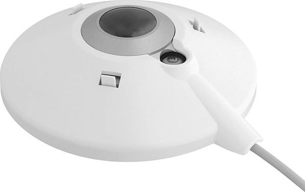
FIGURE 10.4 The Kipp & Zonen CG 4 is constructed to minimize the difference in temperature between the dome and pyrgeometer body. This has the effect of removing the last term of Equations 10.3 to 10.5 and making the measurement problem simpler.
In both comparisons better agreement among the pyrgeometers for outdoor measurements was realized using the calibrations based on the sky-scanning radiometer than using calibrations performed on all of the instruments using a good black-body calibration system. In turn, the uniform black-body calibration on the instruments provided better agreement among the pyrgeometers than using calibrations that came with the instruments either from the manufacturer or their own laboratories. In these studies the measurements were also compared to infrared models of the atmosphere including MODTRAN (Berk et al., 2000) and the line-by-line radiative transfer model (LBLRTM) (Clough, Iacono, and Moncet, 1992). Both models were slightly low with respect to pyrgeometer and scanning radiometer measurements; however, neither model included the effects of aerosols because no aerosol measurements in the infrared were made that could be used as inputs to these models. Any aerosol effect would have likely improved the agreement, but it is not clear by how much. In summary, black-body-calibrated, sky-scanner-calibrated measurements, and models of downwelling infrared irradiance agreed to within 1–2 Wm–2 at night.
The improvement in the agreement when the pyrgeometer calibrations were obtained using the sky scanner versus the black body can be plausibly explained when we consider the spectral response of the pyrgeometer and the spectral distribution of the downwelling infrared. From Figure 10.1 it is clear that spectral infrared sky irradiance is not that of a black body. From Figure 10.3 it is clear that the filters that transmit infrared are not uniform with wavelength. The product of the filter transmission and black-body emission would be expected to be different from the product of the filter transmission and the sky emission leading to the differences seen in the IPASRC results when black-body calibrations were used versus sky-scanner calibrations.
The previous discussion of the absolute sky scanner and improvement in infrared measurements made with pyrgeometers using sky-scanner calibrations suggested a methodology to improve the standard for infrared measurements. The interim World Infrared Standard Group (WISG) for the pyrgeometer infrared standard (http://www.pmodwrc.ch/pmod.php?topic=irc) consists of four pyrgeometers: an Eppley PIR and a Kipp & Zonen CG 4 that participated in both IPASRCs plus another of each type of these pyrgeometers that were calibrated using these two IPASRC participant pyrgeometers.
The current best practice for calibrating pyrgeometers is by outdoor comparison to this standard group (WISG) or, alternatively, by outdoor comparison to pyrgeometers that have been calibrated at the World Radiation Center in Davos referenced to the WISG. Regressions may be performed using any of Equations 10.3 to 10.5. Alternatively, Reda et al. (2006) demonstrated a pyrgeometer calibration method where the nighttime atmosphere is used as the infrared reference.
Julian Gröbner, who is now responsible for the WISG at the World Radiation Center, is developing an absolute pyrgeometer that has been compared to WISG (Groebner, 2012). The comparisons are quite close and indicate that there may be room for slight improvements to the infrared standard, as it exists. Ibrahim Reda, at the National Renewable Energy Laboratory, in collaboration with colleagues at the National Institute of Standards and Technology and Labsphere, has developed a new Absolute Cavity Pyrgeometer (ACP) to measure IR irradiance with traceability to the international system of units (Reda, Zeng, Scheuch, Hanssen, Wilthan, Meyers et al., 2012). The radiation measurement community recognizes the importance of combining the design experiences of multiple sources to ultimately improve the international measurement references.
10.5 Other Pyrgeometer Manufacturers
There are other pyrgeometer manufacturers, but the previous discussion covers the two basic designs for a commercially available pyrgeometer. Other commercial pyrgeometers known to the authors are the Kipp & Zonen CG 3, which differs from the CG 4 in that the field of view of the CG 3 is 150° as opposed to 180°. Hukseflux makes the IR02 pyrgeometer that is based on a PT100 temperature sensor with a 150° field of view (http://www.hukseflux.corn/products/radiationMeasurement/ir02_pyrgeometer.xhtml). EKO Instruments Co., Ltd. makes the MS–202 pyrgeometer, which appears to function much like the Eppley PIR including circuitry to compensate for radiation loss from the exposed junction of the thermopile (the σTB4 in Equation 10.4). However, thermistors or, alternatively, platinum resistance thermometers, to measure the body and dome temperatures are available as options.
10.6 Operational Considerations
Figure 10.5 is a photograph of three Eppley PIRs in ventilated housings. The three pyrgeometers are mounted on an automatic solar tracker to keep the instruments shaded from the direct solar beam at all times of the day. This is the preferred way to operate a pyrgeometer, ventilated and shaded (McArthur, 2004). The ventilation, with optional heating, helps prevent dew and frost formation and keeps the dome cleaner than it would be without ventilation. Shading with a tracking ball or disk minimizes the effects of shortwave leaks associated with the interference filter cut-on wavelength and with possible pinholes in the interference filter, plus the heating of the dome by sunlight is kept to a minimum. Operating without a shaded pyrgeometer will, as expected, result in more uncertainty for the daytime measurements.
Two (for CG 4-type instruments) or three (for PIR-type instruments) voltages need to be measured from a pyrgeometer, and one (CG 4) or two (PIR) voltages need to be supplied to excite the thermistor circuits used for temperature measurements. The thermopile voltage is produced by a temperature difference between the exposed and unexposed junctions of the thermopile. This cumbersome language (exposed and unexposed) is substituted for the usual terms hot and cold junctions because of the reversal of the roles these junctions play in the pyrgeometer relative to their usual use in temperature measurements.
The unexposed junction is at the body temperature of the pyrgeometer, and the exposed junction is generally at a lower temperature because it is cooled by exposure to the dome that radiates to the colder sky. This results in a negative voltage output from the thermopile most of the time. In fact, a good test to verify that the thermopile is connected correctly is to briefly cover the dome with your warm hand and watch the signal become positive.
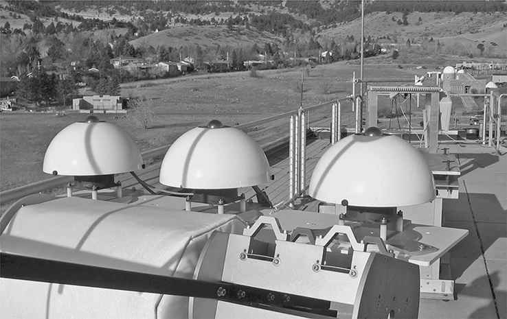
FIGURE 10.5 (See color insert.) Three Eppley PIR pyrgeometers operated in the optimum manner; the instruments are continuously shaded from direct sunlight using an automatic tracker and are placed in heated ventilators to minimize dew formation and dust deposition on the instrument domes.
The thermistor circuit typically used (rarely are platinum resistance thermometers used for these measurements) to measure the temperature of the body and dome may differ in the thermistors used, but most use a configuration similar to that in Figure 10.6. The thermistor’s resistance has a reproducible behavior with temperature. Slight imperfections in thermistor resistance versus temperature are included in the calibration coefficients (k’s) in Equations 10.3 to 10.5. The equations and algebra in FIGURE 10.6 permit the temperature of the dome and body to be determined. For the CG 4 there is only one thermistor for the body temperature, since the manufacturer asserts that the dome and case are nearly the same temperature and does not normally supply a dome thermistor. In support of this claim, Marty et al. (2003) suggested that the dome and body temperature difference term is 20 times smaller for the CG 4 than it is for an Eppley PIR. In an unpublished study, Ellsworth Dutton (personal communication) finds that more than 95% of these dome-body corrections for the PIR are smaller than 30 Wm–2; this suggests that the CG 4 may have a bias, but it is less than 1.5 Wm–2.
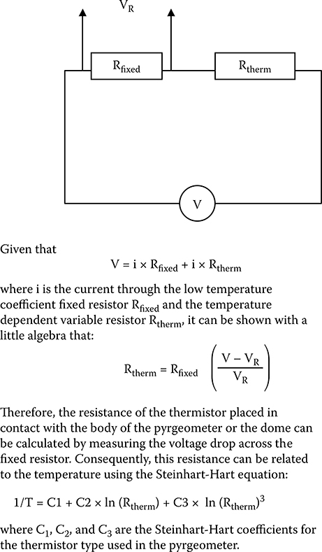
FIGURE 10.6 One method to derive the dome or pyrgeometer body temperatures using a thermistor circuit.
Philipona et al. (2001) and Reda et al. (2012) provide guidance on the uncertainty of pyrgeometer measurements. The uncertainty depends on the provider of the calibration, the formula used to reduce the data to irradiances, and whether a calibration is from a black body or from a comparison to the WISG infrared standard. Furthermore, daytime uncertainties are generally twice the nighttime uncertainties. Philipona et al. (2001) show that the nighttime 95% level of confidence uncertainties range from 0.8 to 4.6 Wm–2 and daytime uncertainties range from 1.6 to 8.2 Wm–2. The uncertainty of the WISG needs to be included in the total estimated uncertainty, which is estimated to be approximately ±1.7 Wm–2 (Julian Gröbner, head of the infrared radiometry section of the World Radiation Center, personal communication). Adding these uncertainties as the square root of the sums of the square implies nighttime uncertainties between 1.9 and 4.9 Wm–2 and daytime uncertainties between 2.3 and 8.4 Wm–2 depending on the calibration procedure followed.
Questions
What distinguishes a black body from a gray body?
At about what central wavelength is the atmospheric window that keeps a clear atmosphere from resembling a perfect black body?
What is the shortest wavelength that typical pyrgeometer domes transmit?
What is the current working calibration standard for broadband infrared radiation?
Why is the thermopile signal from a pyrgeometer only rarely positive?
Why are two temperature measurements required for the Eppley PIR and only one for the Kipp & Zonen CG 4?
A human body should emit like a black body at what temperature?
Why do the best daytime measurements of infrared use a sun-shaded instrument?
References
Albrecht, B. and S. K. Cox. 1977. Procedures for improving pyrgeometer performance. Journal of Applied Meteorology 16:188–197.
Albrecht, B., M. Poellot, and S. K. Cox. 1974. Pyrgeometer measurements from aircraft. Review of Scientific Instruments 45:33–38.
Berk, A., G. P. Anderson, P. K. Acharya, J. H. Chetwynd, L. S. Bernstein, E. P. Shettle, M. W. Matthew, and S. M. Adler-Golden. 2000. Modtran4 user’s manual. Air Force Res. Lab., Space Vehicle Dir., Air Force Mater. Command, Hanscom Air Force Base, MA.
Clough, S. A., M. J. Iacono, and J.-L. Moncet. 1992. Line-by-line calculations of atmospheric fluxes and cooling rates: Application to water vapor. Journal of Geophysical Research 97:15761–15785.
Dutton, E. G. 1993. An extended comparison between LOWTRAN7-computed and observed broadband thermal irradiances: Global extreme and intermediate surface conditions. Journal of Atmospheric and Oceanic Technology 10:326–336.
Eppley Laboratory, Inc. 1995. Blackbody calibration of the precision infrared radiometer, model PIR. Tech. Procedure 05. Available from Eppley Laboratories, P.O. Box 419, Newport, RI 02840.
Fairall, C. W., P. O. G. Persson, E. F. Bradley, R. E. Payne, and S. P. Anderson. 1998. A new look at calibration and use of Eppley precision infrared radiometers. Part I: Theory and application. Journal of Atmospheric and Oceanic Technology 15:1229–1242.
Feltz, W. F., W. L. Smith, H. B. Howell, R. O. Knuteson, H. Woolf, and H. E. Revercomb. 2003. Near-continuous profiling of temperature, moisture, and atmospheric stability using the atmospheric emitted radiance interferometer (AERI). Journal of Applied Meteorology 42:584–597. doi: 10.1175/1520–0450
Groebner, J. 2012. A transfer standard radiometer for atmospheric longwave irradiance measurements. Meteorologia 49: S 105-S111. doi: 10.1088/0026–1394/49/2/S 105.
Knuteson, R. O., H. E. Revercomb, F. A. Best, N. C. Ciganovich, R. G. Dedecker, T. P. Dirkx, S. C. Ellington, W. F. Feltz, R. K. Garcia, H. B. Howell, W. L. Smith, J. F. Short, and D. C. Tobin. 2004a. Atmospheric emitted radiance interferometer. Part I: Instrument design. Journal of Atmospheric and Oceanic Technology 21:1763–1776.
Knuteson, R. O., H. E. Revercomb, F. A. Best, N. C. Ciganovich, R. G. Dedecker, T. P. Dirkx, S. C. Ellington, W. F. Feltz, R. K. Garcia, H. B. Howell, W. L. Smith, J. F. Short, and D. C. Tobin. 2004b. Atmospheric emitted radiance interferometer. Part II: Instrument performance. Journal of Atmospheric and Oceanic Technology 21:1777–1789.
Marty, C., R. Philipona, J. Delamere, E. G. Dutton, J. Michalsky, K. Stamnes, R. Storvold, T. Stoffel, S. A. Clough, and E. J. Mlawer. 2003. Downward longwave irradiance uncertainty under arctic atmospheres: Measurements and modeling. Journal of Geophysical Research 108:4358–43669. doi:10.1029/2002JD002937
McArthur, L. J. B. 2004. Baseline Surface Radiation Network (BSRN). Operations Manual. WMO/ TD-No. 879, World Climate Research Programme/World Meteorological Organization.
Payne, R. E. and S. P. Anderson. 1999. A new look at calibration and use of Eppley precision infrared radiometers. Part II: Calibration and use of the Woods Hole Oceanographic Institution improved meteorology precision infrared radiometer. Journal of Atmospheric and Oceanic Technology 16:739–751.
Philipona, R. 2001. Sky-scanning radiometer for absolute measurements of atmospheric long-wave radiation. Applied Optics 40: 2376–2383
Philipona, R., E. G. Dutton, T. Stoffel, J. Michalsky, I. Reda, A. Stifter, P. Wendling, N. Wood, S. A. Clough, E. J. Mlawer, G. Anderson, H. E. Revercomb, and T. R. Shippert. 2001. Atmospheric longwave irradiance uncertainty: Pyrgeometers compared to an absolute sky-scanning radiometer, atmospheric emitted radiance interferometer, and radiative transfer model calculations. Journal of Geophysical Research 106:28129–28141.
Philipona, R., C. Fröhlich, and C. Betz. 1995. Characterization of pyrgeometers and the accuracy of atmospheric long-wave radiation measurements. Applied Optics 34:1598–1605.
Philipona, R., C. Fröhlich, K. Dehne, J. Deluisi, J. A. Augustine, E. G. Dutton, D. W. Nelson, B. Forgan, P. Novotny, J. Hickey, S. P. Love, S. Bender, B. McArthur, A. Ohmura, J. H. Seymour, J. S. Foot, M. Shiobara, F. P. J. Valero, and A. W. Strawa. 1998. The baseline surface radiation network pyrgeometer round-robin calibration experiment. Journal of Atmospheric and Oceanic Technology 15:687–696.
Reda, I., J. R. Hickey, J. Grobner, A. Andreas, and T. Stoffel. 2006. Calibrating pyrgeometers outdoors independent from the reference value of the atmospheric long-wave irradiance. Journal of Atmospheric and Solar-Terrestial Physics 68:1416–1424.
Reda, I., J. R. Hickey, T. Stoffel, and D. Myers. 2002. Pyrgeometer calibration at the National Renewable Energy Laboratory (NREL). Journal of Atmospheric and Solar-Terrestial Physics 64:1623–1629.