12 Solar Spectral Measurements
I shall without further ceremony acquaint you that in the year 1666, I procured me a triangular glass prism, to try therewith the celebrated phenomena of colors.
Sir Isaac Newton
(1642–1727)
12.1 Introduction
Solar radiation is not uniformly distributed in wavelength. The spectral distribution of solar radiation as it arrives at the top of the atmosphere is equivalent to a blackbody spectrum with an effective temperature of 5777 K that is modified by selective absorption and emissions in the sun’s own atmosphere. This radiation is further and significantly modified by scattering and absorption processes as it passes through the earth’s atmosphere before it reaches the surface.
This chapter begins with a discussion of the extraterrestrial solar spectrum and its modest variability with the 11-year solar cycle. Its variability with sun–earth distance is covered in Chapter 2. Clear-sky interactions of solar radiation with the atmosphere are also discussed in this chapter including molecular, or Rayleigh, scattering, aerosol scattering and absorption, and absorption by atmospheric gases. Scattering and absorption by clouds is a very complex topic and is not addressed in this handbook. The authors suggest the textbook by Liou (1992) for an introduction to this subject.
Some useful broadband spectral measurements including photometric, photosynthetically active radiation (PAR), and ultraviolet photometry are covered in this chapter. A discussion of narrowband photometry follows with a focus on its use in retrieving aerosol optical depth and water vapor (the most important clear-sky constituents affecting the spectral distribution of solar radiation at the earth’s surface). Instruments for making these measurements are then described with some advice on the specifications to consider if purchasing these instruments. The chapter concludes with brief sections on moderate spectral resolution spectrometry and moderate resolution spectral irradiance models.
12.2 The Extraterrestrial Solar Spectrum
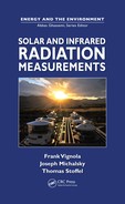
The solar spectrum covers a wide wavelength range; however, for practical purposes virtually all of the sun’s energy that reaches the earth’s surface lies between the wavelengths of 280 and 4000 nm. Figure 12.1 is a plot of the spectral irradiance in W/(m2-nm) versus wavelength in nm (Gueymard, 2004). The integral of this spectral distribution over all wavelengths, if measured just above the earth’s atmosphere for one 11-year solar cycle, yields 1366 W/m2 at the mean distance between the sun and the earth (149,597,887 km or 92,955,818 miles). This mean distance is defined as one astronomical unit (1 AU). Fröhlich (2006) summarized how extraterrestrial irradiance has varied over the last two 11-year solar cycles. The maximum to minimum solar cycle variation averages about 0.1% of the total energy with short-term excursions about three times this amount. The total irradiance monitor (TIM) on the Solar Radiation and Climate Experiment (SORCE) satellite (Rottman, 2005), however, measured a smaller mean value for the integrated spectral irradiance at 1 AU of 1361 W/m2. To date these differences, which are statistically significant, have not been completely resolved (Kopp and Lean, 2011; Kopp, Fehlman, Finsterle, Harber, Heureman, and Wilson, 2012).
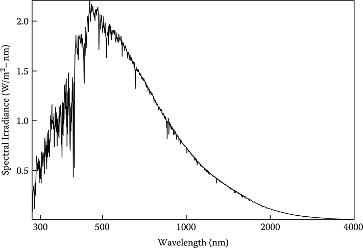
FIGURE 12.1 Extraterrestrial solar spectral irradiance distribution at mean sun–earth distance.
Harder, Fontenla, Pilewskie, Richard, and Woods (2009) used the solar irradiance monitor (SIM) on the SORCE satellite to investigate the variations in portions of the solar spectrum. Separately assessing the variability in the spectral bands from 201–300, 300–400, 400–691, 691–972, 972–1630, and 1630–2423 nm, they found maximum changes of about 0.6 Wm–2 with the largest changes in the shortest wavelength bands. The measurements spanned a period of only 4 years or about one-half of the maximum change in total irradiance expected over a solar cycle; however, even twice this change would amount to a small fraction of 1 Wm–2 by the time the radiation reaches the surface of the earth. Consequently, it is reasonable to assume that the sun’s inherent variability is lower than can reasonably be detected at the surface given the scattering and absorption that occurs within the earth’s atmosphere. These interactions with the earth’s atmosphere are discussed in the next section.
12.3 Atmospheric Interactions
When solar radiation passes through the atmosphere, complex interactions occur depending on the wavelength of the radiation and the composition of the atmosphere at the time. More specifically, solar radiation either passes unscathed to the surface, or it is scattered or absorbed by molecules, aerosols, cloud water droplets, and ice crystals.
12.3.1 RAYLEIGH SCATTERING
Molecular scattering is the elastic scattering of solar radiation by the molecules in the atmosphere first explained by Lord Rayleigh (1871). Many papers have been written describing the scattering of solar radiation by molecules, but it is not a dead subject (Eberhard, 2010). Bodhaine, Wood, Dutton, and Slusser (1999) thoroughly examined the problem of calculating the molecular scattering optical depth as a function of wavelength. Optical depth, in general, is a measure of the wavelength dependent extinction (by scattering or absorption) that occurs as a beam of radiation propagates through a medium. It can be defined using
where I0 is the strength of the source (e.g., the spectral solar irradiance) before it enters the atmosphere, I is the strength after it has passed through the atmosphere to the surface, τ is the optical depth in a vertical path, m is the amount of atmosphere traversed relative to the vertical path, and λ is wavelength. A good approximation to optical depth by Rayleigh scattering is given by Hansen and Travis (1974):
where wavelength λ is in pm, P is the pressure at the measurement site within the earth’s atmosphere in kilopascals, and P0 is the standard pressure at sea level equal to 101.325 kilopascals (100 kilopascals = 1000 millibars). It is evident from examining Equation 12.2 that Rayleigh scattering is most effective in the shortest wavelengths of the solar spectrum and decreases dramatically at longer wavelengths (approximately as λ–4). It is also evident that at higher elevations there is less Rayleigh scattering because of lower atmospheric pressure.
12.3.2 AEROSOL SCATTERING AND ABSORPTION
Aerosols are always present in the atmosphere. They manifest themselves as the haze often noticed when looking toward the horizon. Generally, aerosols are concentrated near the surface but may appear in layers especially when transported into a region from long distances. When volcanic eruptions occur that are strong enough to inject dust and gases into the stratosphere, such as Mount Pinatubo did in 1991, a stratospheric aerosol layer may persist for years from the sulfur gases that are chemically transformed into aerosols (see Figure 4.9). The dust particles from an eruption, however, are large and therefore are removed from the atmosphere quickly because of gravitational settling. Figure 12.2 is the long-term record of transmission from Mauna Loa Observatory. The largest excursions are caused by the three named volcanic eruptions. Lower transmission persists for years after the events.
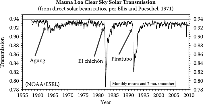
FIGURE 12.2 Transmission record from Mauna Loa Observatory. The large dips in transmission are associated with stratospheric aerosols from three volcanoes. Note that the transmission is suppressed for around three years after the initial eruptions.
Aerosols are capable of both scattering and absorbing solar radiation depending on their chemical makeup and on the wavelength of the incident solar radiation. The probability of a photon scattering from an aerosol is called the single scattering albedo, ϖ0. Often ϖ0 exceeds 0.9 at visible wavelengths for typical continental aerosols. For sea salt aerosols, ϖ0 is close to 1.0 at visible wavelengths. The term co-albedo is used for the quantity (1 - ϖ0) and is the probability of the photon being absorbed upon encountering an aerosol. Therefore, sea salt aerosols would have a coalbedo of zero in the visible spectral region. Another quantity that describes the scattering of aerosols is the asymmetry parameter, often denoted g. The probability of scattering in any given direction is given, approximately, by the Henyey–Greenstein function (Henyey and Greenstein, 1941):
where θ is 0° in the direction of photon propagation and 180° in the opposite direction. This probability function exhibits these properties:
The larger g is, the more the scattering into the forward hemisphere. A g value of zero would imply isotropic scatter or equal probability of scattering in all directions. Typical values of g are between 0.5 and 0.7 for continental aerosols. Sea salt aerosols tend to be large and have large values of asymmetry parameter, while anthropogenic pollution aerosols are small with lower asymmetry parameters. The use of these two parameters ϖ0 and g as inputs to spectral models of solar radiation is discussed in Section 12.6.2.
12.3.3 GAS ABSORPTION
The dominant gas absorber affecting the spectral distribution of the incident solar irradiance in the solar spectrum is water vapor with several major absorption bands in the near-infrared. For example, Figure 2.15 indicates the strong water vapor absorption band in the global horizontal irradiance (GHI) spectrum centered near 940 nm. This is of particular importance to many solar photovoltaic (PV) collectors since the peak response of crystalline silicon PV is near the strong water vapor band around 940 nm. Ozone is another important absorber in the atmosphere. However, its strongest absorption is below 380 nm in the Hartley–Huggins bands. The Chappuis ozone band is broad but has modest absorption centered near 610 nm. The Wulf bands in the near-infrared are even less absorbing. Other gases such as O2 and CO2 are ever-present but less significant in the sense that they do not remove a large fraction of the total solar radiation. Nitrogen dioxide (NO2) is an important gas when air pollution concentrations are high. This gas produces a reddish-brown tinge to the skylight by preferentially absorbing blue solar radiation. The major production of NO2 is by motor vehicles, which is also the main source of ozone production in cities that exceed the U.S. Environmental Protection Agency (EPA) standards for this molecule.
Optical depths associated with ozone absorption τozone may be calculated using
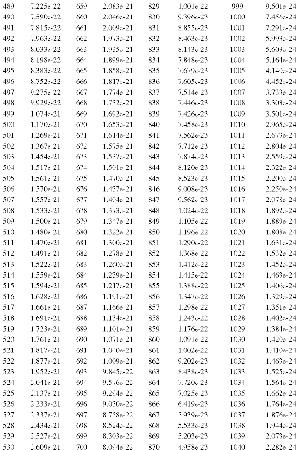
where ηozone is the ozone abundance, and αozone is the ozone absorption coefficient. Typically, for midlatitudes, the ozone column (the amount of ozone present from the surface to the top of the atmosphere) is in the neighborhood of 300 Dobson units but varies typically between 200 and 400 Dobson units. A Dobson unit (DU) of ozone is equal to 2.687 x 10¹⁶ molecules per cm2. This is 1/1000 of Loschmidt’s number, or the number of molecules in a cubic centimeter of a gas under standard temperature and pressure. A typical value of 300 DUs of ozone at the standard temperature of 273.15 K and standard pressure of 101.325 kilopascals would form a column of ozone 0.3 cm high. Current ozone data from NASA’s Ozone Monitoring Instrument (OMI) satellite are posted on the NASA website (http://toms.gsfc.nasa.gov/teacher/ozone_overhead_v8.xhtml) 1 or 2 days after they are acquired. Ozone absorption coefficients αozone in units of molecules–1 at 1 nm resolution between 407 and 1086 nm for the visible and near-infrared (Chappuis and Wulf bands, respectively) based on Shettle and Anderson (1995) are given in Table 12.1. As an example, using Equation 12.6 we find that 300 DU will yield a vertical optical depth at 602 nm of
TABLE 12.1
Ozone Absorption Coefficients (molecules–1) @ the Given Wavelengths (nm)
|


12.3.4 TRANSMISSION OF THE ATMOSPHERE
Figure 12.3 illustrates the transmission of direct solar (beam) irradiance for the parameters given in the legend. Superimposed on the plot is the spectral irradiance (dot-dash line) for the given trace species with the sun in the zenith position at 1 AU The Rayleigh scattering is a smooth function of wavelength and the larger dips (and many of the smaller ones) that depart from this smooth function result from mixed gas absorption by O2 and CO2. Water vapor (light gray) and ozone (dark gray) absorption bands are plotted separately. Even a modest aerosol optical depth (dashed line) of 0.15 at 500 nm with a wavelength dependence given by
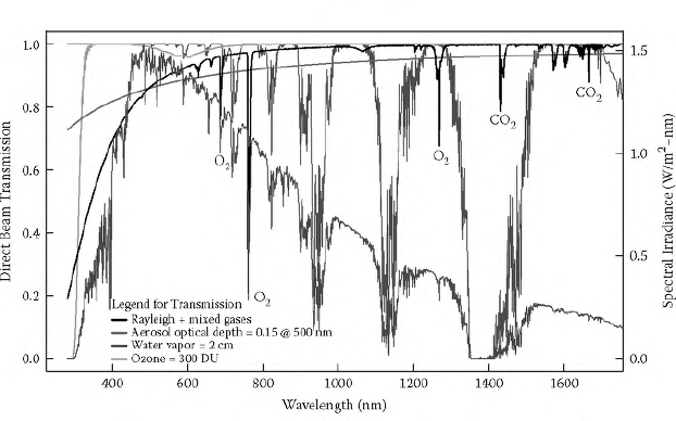
FIGURE 12.3 (See color insert.) Direct solar transmission of major components of the clear-sky atmosphere (left axis); superimposed on the transmission spectra is the spectral irradiance calculated for these conditions (right axis). (See color insert for clearer separation of curves.)
where β = 0.06092, and ϖ = 1.3 gives a reduced transmission that is typically the second most important contributor to solar radiation extinction after Rayleigh scattering. This is true for clear skies because the extinction from aerosols is typically large in the midvisible wavelengths where solar irradiance is highest. Note that some spectral absorption features in the spectral irradiance curve are not in the transmission spectra. Most of these extra absorption features are from the extraterrestrial solar spectrum and occur in the outer layers of the sun’s atmosphere (see Figure 12.1).
12.4 Broadband Filter Radiometry
There are many reasons to measure isolated portions of the solar spectrum. For example, broadband measurements of red, green, and blue light are used for specifying color for both commercial and artistic reasons. Broadband measurements of the spectral distribution of sunlight can be used for calculating the efficiency of spectrally dependent photovoltaic devices (Michalsky and Kleckner, 1984). Although not the preferred method, broadband filters have been used with a pyrheliometer to approximately measure aerosol optical depths (Dutton and Christy, 1992). In this section we discuss some common types of broadband spectral measurements with solar applications.
12.4.1 PHOTOMETRY
Photometry is the measurement of light that the human eye can sense. Although there have been slight modifications to the definition, the Commission Internationale de l’Eclairage (CIE) defined the basic luminosity function for daytime (photopic) vision for the average human eye in 1924 (CIE, 1926). Figure 12.4 illustrates how the eye response varies with wavelength with a peak near 555 nm. Scotopic response is the wavelength response of the eye in darkened conditions. The response distribution with wavelength is similar but more skewed, and it shifts to shorter wavelengths with the peak response near 507 nm. Since we are mostly interested in daylight applications we will focus only on the photopic response that most photometers are designed to measure.
To convert any spectral irradiance, such as sunlight, into illuminance L, a very good approximation is
where
![]() is the photopic function plotted in Figure 12.3, I(λ) is the spectral irradiance in W/(m2-nm), and L has units of lumens/m2.
is the photopic function plotted in Figure 12.3, I(λ) is the spectral irradiance in W/(m2-nm), and L has units of lumens/m2.
Manufacturers of photometers try to match the photopic function as closely as possible using combinations of filters and detector responses. The success with which this is achieved varies; an example is given in Figure 12.5 from the photometry tutorial offered on UDT’s website (http://www.udtinstruments.com/applications/photometric/photometry.shtml). When searching for a photometer, make sure that your search is for a photometer with a photopic response since the term photometer is used for many types of instruments that do not attempt to match the spectral response of the eye in daylight. If the photometer is to be used outdoors, make certain that it is designed to be waterproof and rugged. Although manufacturers try to match the CIE response curve, they all fail to some extent, so look for a reasonable photopic match. If the goal is to measure solar radiation for daylighting purposes, for example, performing the integral in Equation 12.9 using a modeled clear-sky irradiance first with the photopic function
![]() and then using the manufacturer’s estimate of the photopic function, say
and then using the manufacturer’s estimate of the photopic function, say
![]() ', a bias can be calculated. Most daylight photometers will measure total horizontal illuminance. To do this well, a respectable cosine response for the instrument is required; that is, the signal should fall off approximately as the cosine of the angle of incidence. If the response is within 10% of the normalized response (actual response as a function of incident angle divided by cosine of the incident angle) out to about 80° incidence, then it can be considered acceptable. The left side of Figure 12.6 illustrates an acceptable cosine response for an actual instrument. Some manufacturers may illustrate cosine response as shown on the right side of Figure 12.6, but without the normalized cosine plotted for comparison. These plots may look approximately correct but should be plotted normalized as in the left half of Figure 12.6 for proper evaluation. Other factors to consider are instrument stability (responsivity changes are less than 3% per year) and absolute uncertainty (better than 5%). A final note on cost: It was possible to purchase good photopic photometers for outdoors use for around US$500 in 2010.
', a bias can be calculated. Most daylight photometers will measure total horizontal illuminance. To do this well, a respectable cosine response for the instrument is required; that is, the signal should fall off approximately as the cosine of the angle of incidence. If the response is within 10% of the normalized response (actual response as a function of incident angle divided by cosine of the incident angle) out to about 80° incidence, then it can be considered acceptable. The left side of Figure 12.6 illustrates an acceptable cosine response for an actual instrument. Some manufacturers may illustrate cosine response as shown on the right side of Figure 12.6, but without the normalized cosine plotted for comparison. These plots may look approximately correct but should be plotted normalized as in the left half of Figure 12.6 for proper evaluation. Other factors to consider are instrument stability (responsivity changes are less than 3% per year) and absolute uncertainty (better than 5%). A final note on cost: It was possible to purchase good photopic photometers for outdoors use for around US$500 in 2010.
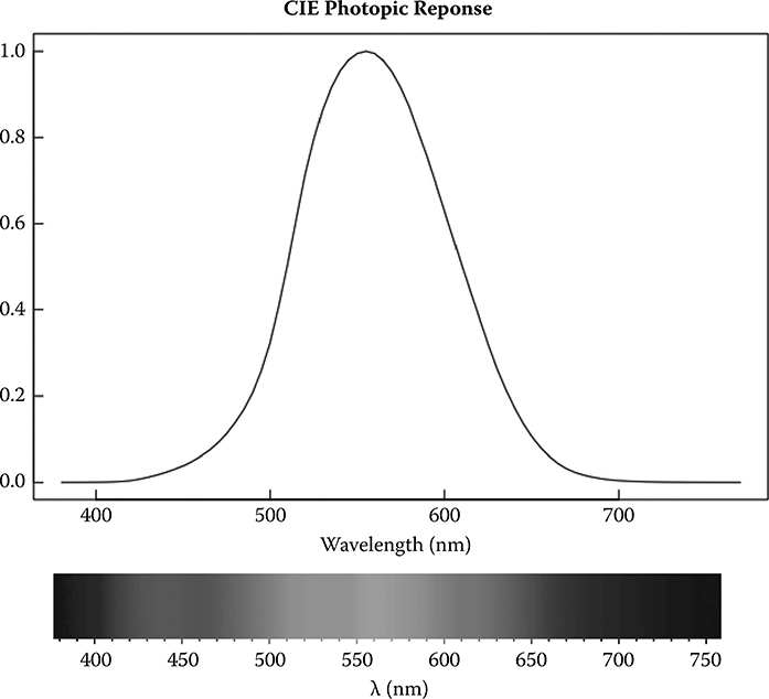
FIGURE 12.4 (See color insert.) The typical human eye’s response for sunlit conditions as specified by the Commission International l’Eclairage (CIE); en.wikipedia. org/wiki/ File:Srgbspectrum.png is the source for the color diagram beneath the photopic response plot.
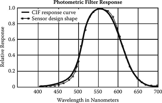
FIGURE 12.5 An example of one manufacturer’s (Macam) attempt to match the CIE photopic response using filters. (From Austin, R., The Guide to Photometry, UDT Instruments, San Diego, CA, n.d. With permission.)
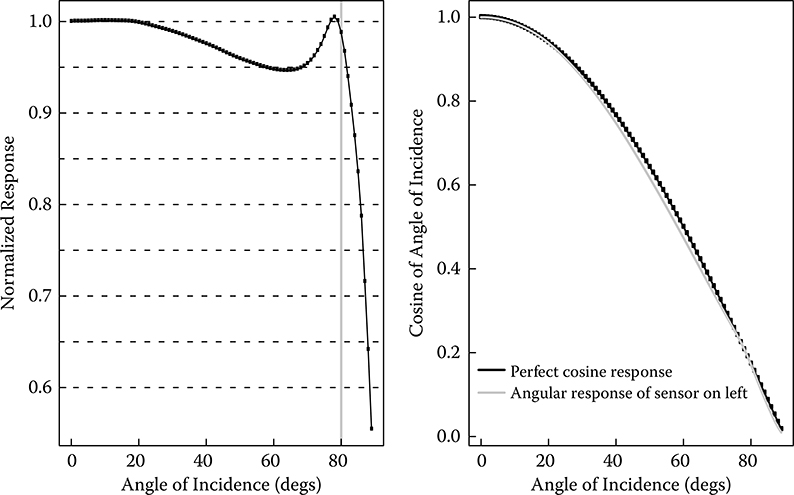
FIGURE 12.6 An example of the cosine response of a good receiver compared with an exact cosine response plotted normalized and unnormalized.
12.4.2 PHOTOSYNTHETICALLY ACTIVE RADIATION (PAR)
Plants use PAR to transform water and carbon dioxide into sugars and oxygen through photosynthesis. PAR is measured with sensors that filter light to accept radiation between about 400 and 700 nm. Plants mostly use the light near either end of this wavelength range for photosynthesis and reflect more of the green light, thus giving plants their color. Photosynthesis is a quantum process. In other words, photons cause the reactions that occur in plants; therefore, it would seem logical to define PAR in terms of photons per unit time per unit area. If we know the spectral distribution of sunlight as a function of wavelength I(λ), say in W/(m2-nm), and the energy of a photon is given by hc/λ in joules, then the photosynthetic photon flux density (PARpppd) in units of photons/(sec-m2) can be calculated as
where hc is the product of Planck’s constant and the speed of light, respectively. To make the numbers reasonably convenient to work with, the photon number is usually expressed in units of micromoles 6.022 × 10¹⁷. PAR with full sun (e.g., broadband DNI = 1000 W/m2) on a cloudless summer day would measure around 2000 μmoles/ (m2-sec). PAR is sometimes defined by
PAR, in this case, is simply the integrated energy in W/m2 between the wavelengths of 400 and 700 nm. Clearly, the two equations are different. Figure 12.7 illustrates the different spectral weighting. For the energy definition of PAR, the entire energy spectrum in the wavelength interval between 400 and 700 nm is given equal weighting illustrated by the thin black line. For the photosynthetic photon flux density (PPFD) definition in Equation 12.10, weighting is proportional to the wavelength. A 400 nm photon has more energy than a 700 nm photon, yet both produce a chemical reaction in plants; therefore, an energy spectrum should be weighted by the dashed curve in Figure 12.7 to calculate its photosynthetic effect. Federer and Tanner (1966) and Biggs, Edison, Eastin, Brown, Maranville, and Clegg (1971) began to standardize PAR measurements with some early sensor designs that attempted to weight the sensitivity proportionally to the wavelength. For example, LI-COR Biosciences and Kipp & Zonen are two instrument manufacturers with sensor designs, the LI–190 and PAR Lite, respectively, that approximate this weighting function using colored glass or interference filters in combination with the silicon photodiode detector to achieve proper wavelength sensitivity. Other considerations in purchasing a PAR sensor, besides the agreement between the theoretical and actual photosynthetic response (dashed line in Figure 12.6), are all-weather ruggedness, good cosine response, and calibration stability. An annual stability of better than 3% and an absolute response of better that 5% are reasonable specifications to expect. Good PAR sensors could be found for about US$500 in 2010.

FIGURE 12.7 The weighting for PAR measured in energy units of W/m2 (thin black line) and for weighting in photons/(sec-m2) (thick dashed line).
12.4.3 UVA AND UVB
Ultraviolet (UV) radiation has wavelengths below 400 nm and above 10 nm. The practical lower wavelength limit for the UV for solar radiation at the earth’s surface is around 290 nm since ozone in the stratosphere absorbs virtually all of the radiation below this wavelength. High spectral resolution measurements of the solar UV spectrum require a spectrometer with two dispersive elements to minimize stray light from the stronger and longer wavelength portion of the solar spectrum if one is to achieve the best measurements at the very important shortest UV wavelengths. Because of the high cost of a double monochromator, it is more common to measure UV in broad wavelength bands. UVA covers the wavelengths between 315 nm and 400 nm and UVB covers the wavelengths between 290 nm and 315 nm. UVC includes wavelengths shorter than 290 nm but will not be discussed here because no significant amounts of UVC reach the earth’s surface due to atmospheric absorption and scattering.
UVB is the most common UV measurement because of its deleterious effects on humans and material properties. Overexposure to UVB is associated with sunburn, eye disease (including cataracts), and suppression of the immune system. However, underexposure to UVB leads to lower vitamin D production, which has deleterious effects as well. Exposure to UVB at levels before sunburn may produce a net positive effect (Holick, 2005). The World Health Organization (WHO) has, however, taken the conservative position on its website (http://www.who.int/uv/faq/uvhealtfac/en/index.xhtml) that the harmful effects of UVB exposure generally outweigh the positive ones.
UVA radiation penetrates deeper into the skin layers and causes premature aging. It also produces hydroxyl and oxygen radicals that cause DNA damage. In fact, some scientists believe that the higher incidence of malignant melanomas in sunblock users may result from sunblock ingredients blocking UVB but not UVA (Autier, Dore, Schifflers, Cesarini, Bollaerts, Koelmel et al., 1995).
UVB sensors are usually tailored to match as closely as possible the Diffey erythemal response function (McKinlay and Diffey, 1987). UVA sensors measure the 315–400 nm passband with a uniform response. Most modern UVB and UVA sensors use a filter to define the passband of the radiation that one wishes to isolate followed by a phosphor that is sensitive to UV. The phosphor produces visible radiation that is more easily detected by solid-state detectors. For these instruments to perform well and with good stability at the expected low signal levels, they must be temperature stabilized. Another important consideration is their ability to approximate a Lambertian cosine response; that is, they should mimic a receiver with a perfect cosine angular response as described in the section on photometry. As far as absolute accuracy, UVB sensors that are better than 10% are likely the best that one can expect; relative calibration stability should be better than 5% per year. A list of UVB instrument manufacturers (see Appendix F) generally includes EKO Instruments, Kipp & Zonen, Solar Light, and Yankee Environmental Systems, Inc.
12.5 Narrow-Band Filter Radiometry
Narrow-band filter radiometers are used for the measurement of atmospheric aerosol and molecular constituents, such as water vapor and ozone. Direct normal solar irradiance instruments are called sun photometers or, more generally, sun radiometers since they are used outside the photopic response band as well as within it. A sun radiometer measures in several narrow wavelength bands with responsivities defined by full widths (wavelength) at half-maximum (response) of 5–10 nm. The instrument should track the sun using a narrow field of view to observe the disk of the sun plus a small annulus around the sun that allows for tracking uncertainty and atmospheric refraction (e.g., 2° to 2.5° full view angle).
12.5.1 AEROSOL OPTICAL DEPTH
For a clear view of the sun with no clouds, one can use Beer’s law to calculate the column aerosol optical depth using
where Equation 12.12 is Equation 12.1 expanded to explicitly show the optical depth components that are normally measured in the visible and near-infrared spectrum. For sun radiometers to measure aerosols, filter wavelengths and bandwidths are carefully chosen to avoid water vapor and molecular oxygen absorption bands. If I(λ) is measured, the m’s calculated using the sun’s elevation, τozone obtained from satellite or ground-based measurements, τRayleigh calculated using Equation 12.2 and the atmospheric pressure is measured, then τaerosol can be calculated if Io(λ) is known. Determining of the extraterrestrial solar irradiance, Io(λ), is the crux of the matter when it comes to performing good sun radiometry and is the most demanding task in making valid aerosol optical depth measurements. For example, a 1% uncertainty in Io(λ) leads to an approximate uncertainty of 0.01 in aerosol optical depth.
The air masses for ozone, aerosol, and Rayleigh scattering differ because each is vertically distributed differently in the earth’s atmosphere. However, an adequate approximation for many purposes is to assume that the air masses for ozone, aerosol, and Rayleigh scattering are the same, in which case Equation 12.13 reverts to Equation (12.1). If we take the natural logarithm of Equation 12.1 we get
that has the form of a linear equation y = yo + b. x. If we plot ln(I) versus air mass m, then for a perfectly stable atmosphere we should get a straight line whose intercept is the ln(Io) and whose slope is the negative of the total optical depth. If we now know ln(Io), then we can calculate or measure everything else in Equation 12.13 to derive total optical depth at any other time. Subtracting optical depths caused by Rayleigh scattering and ozone absorption yields the aerosol optical depth.
Although we have assumed that the air masses are the same for the different extinction components to illustrate this Langley plot technique, the more correct procedure for Langley analysis is to plot the left-hand side of the following equation versus aerosol air mass, that is,
Using Equation 12.13 versus Equation 12.14 for the determination of the Langley intercept results is much less than 1% bias at visible and longer wavelengths, but it becomes crucial to use Equation 12.14 for studies in the ultraviolet because Rayleigh and ozone are generally the dominant contributions to the total optical depth.
The air mass relative to the zenith direction typically used in Equation 12.13 is for a pure Rayleigh atmosphere. Kasten and Young (1989) developed a revised approximation for a Rayleigh atmosphere, namely,
where the solar zenith angle sza on the right-hand side of the equation is in degrees. Almost always it is the case that more than 90% of the atmospheric ozone resides in the stratosphere between 20 and 40 km and varies with season. The ozone layer is lower in the winter than in the summer. The altitude also depends on the latitude with higher layers at the equator than at the poles. If one considers the geometry of an elevated layer, ozone air mass relative to the zenith direction is somewhat smaller than the Rayleigh air mass. Ozone air mass as calculated by the Dobson spectrophotometer community (Komhyr and Evans, 2008) is given by
where R is the mean radius of the earth 6371.299 km, r is the station height above mean sea level in km, and h is the mean height of the ozone layer in km. Although aerosol layers can be elevated, especially as a result of long-range transport in the free troposphere, they typically reside in the boundary layer near the surface. We therefore use the same air mass expression for aerosol that is used for water vapor (Kasten, 1966; based on Schnaidt, 1938), namely,
Two well-known locations for obtaining the clear, stable atmospheres needed for this straightforward determination of ln(Io) are Izaña Observatory on the island of Tenerife in the Canary Islands and at Mauna Loa Observatory on the island of Hawaii in the Hawaiian Islands. Even at these sites, one requires a number of Langley plots using only morning data since upslope winds can bring lower tropospheric air over the site. Examining multiple Langley plots (Langleys) allows one to identify measurement outliers and provides a robust estimate of the uncertainty of the calibration constant ln(Io).
Alternatively, indoor lamp calibrations, in principle, can be used to calibrate sun radiometers. A very careful study of lamp calibrations versus Langley calibrations from a high mountain site (Jungfraujoch in Switzerland) by Schmid and Wehrli (1995) demonstrated that the calibrations differ from as little as 0.2% to as much as 4.1% depending on the wavelength with most filter differences greater than 1.4%. A follow-on study (Schmid, Spyak, Biggar, Wehrli, Skeler, Ingold et al., 1998) suggested that typical differences between the two calibration techniques were at best 2–4% and became more variable than this if different published extraterrestrial spectra (Io(λ)) were used for the extraterrestrial irradiance. Lamp calibration, however, may be a viable means for checking the stability of a calibration, but Langley plots are suggested for establishing the initial calibration of the radiometer. For example, if a good Langley calibration is associated with a near-concurrent lamp calibration, then future lamp calibrations could be used to track and correct for the degradation of the sun radiometer if needed for a site where good Langley plots occur infrequently or are impossible.
Michalsky, Schlemmer, Berkheiser, Berndt, and Harrison (2001) and Augustine, Cornwall, Hodges, Long, Medina, and Delusi (2003) describe two calibration methods that do not require high mountains or lamps. The fundamental idea is to use all possible Langleys to develop a robust and continuously updated calibration of the sun radiometer. These methods have demonstrated uncertainties around 1%.
AERONET and its affiliates form the largest aerosol optical depth network in the world (Holben, Eck, Slutsker, Tanre, Buis, Setzer et al., 1998). This network uses measurements on Mauna Loa to calibrate their standards using Langley plots over several good, stable days. These instruments are then transported to Goddard Space Flight Center in Maryland, where they are used to transfer calibrations to the network instruments via side-by-side comparisons. Recent comparisons between sun radiometers calibrated using this method and the method of Michalsky, Schlemmer et al. (2001) found biases in daily-averaged aerosol optical depths of less than 1% over a 3-year period (Michalsky, Denn et al. 2010).
12.5.2 WATER VAPOR
Using narrow-band filter radiometers to measure water vapor is more difficult than measuring aerosol optical depth. Thome, Herman, and Reagan (1992) reviewed the sun radiometric techniques, both empirical and theoretical, that had been used in the previous 80 years for water vapor column retrievals. The technique that has been used most often in the last 20 years to retrieve water vapor is based on the modified Langley method first introduced by Reagan, Thome, Herman, and Gall (1987). If measurements are made in the water vapor band, then Equation 12.1 can be modified; thus
where τ and m are the optical depths associated with Rayleigh scattering and aerosol scattering and absorption. TH2O is the transmission in the water band due to water vapor absorption. Bruegge, Conel, Green, Margolis, Holm, and Toon (1992) modeled the transmission in the water band using
where k and b are constants. This accounts for the product of water vapor air mass m and column water u not behaving linearly in extinction. In other words, while doubling aerosol doubles aerosol optical depth, doubling water vapor increases the water vapor optical depth by about a factor of
 . Although Reagan et al. (1987) used the approximation that b was equal to 0.5, it should be calculated for the specific filter used for the measurements because the optical depth is measured over a finite filter width of, typically, 10 nm and includes water vapor and water vapor continuum contributions. A radiative transfer model is used to calculate the transmission over the expected range of u. m. Each calculated transmission value t(λ) for a given water vapor path is formed by convolving with the filter function f(λ) according to
Taking the natural logarithm of Equation 12.19 twice and rearranging terms gives
A plot of the left-hand side versus ln(u • m) should be linear, and a linear least-squares fit to the calculations yields the ln(k) and b coefficients. Taking the natural logarithm of Equation 12.18 after substituting Equation 12.19 and rearranging terms yields
If the left-hand side of Equation 12.22 is plotted versus mb on clear days that have stable water vapor, the intercept of the linear plot is ln(Io), which can then be used to solve for water vapor for any subsequent clear-sky measurement. Langley plots for aerosol channels are less of a challenge than modified Langley plots for the water channel. Even seemingly clear days generally experience large water vapor changes; therefore, many more modified Langleys are required to obtain even an approximate calibration compared to the aerosol channels.
AERONET (Holben, Eck et al., 1998) implemented its version of this algorithm to produce a column water vapor product for its sites. Their latest methodology for water vapor retrieval is described in Smirnov, Holben, Lyapustin, Slutsker, and Eck (2004).
Michalsky, Min, Kiedron, Slater, and Barnard (2001) introduced an alternative technique for retrieving water vapor that depends on calibration with a stable spectral lamp and a trusted extraterrestrial spectral irradiance in the vicinity of the 940 nm water vapor band and the continuum near it. Besides the uncertainty in the extraterrestrial spectrum and the lamp calibration, the overall uncertainty of this procedure also depends on estimating the aerosol and Rayleigh scattering optical depths and on the accuracy of the water vapor transmission calculations, as was the case for the previously mentioned modified Langley approach.
If column water vapor is required, for example, for the spectral irradiance model calculations that are described in Section 12.6.2, and a sunradiometer with a water channel is not available, there are other reliable sources of column-integrated water vapor.
The National Weather Service launches radiosondes on balloons twice each day as part of a worldwide network of measurements that profile temperature, humidity, pressure, and wind speed and direction. The launches are coordinated with launch times centered on 0 and 12 GMT. The website http://www.wmo.int/pages/prog/www/ois/volume-a/vola-home.htm contains a list of stations launching radiosondes throughout the world. Although relative humidity is measured on these sondes, dew point temperature is the reported value. The actual vapor pressure e for any measurement in the profile can be calculated from the dew point temperature Td using
The particulars of radiosondes measurements as practiced in the United States are explained in Federal Meteorological Handbook No. 3 (1997, http://www.ofcm.gov/fmh3/text/default.htm). Column water vapor column can then be calculated using
In Equation 12.24 from Fleagle and Businger (1963) W is the integrated water column, g is the acceleration due to gravity, and p is the pressure with the integration between pressure levels p1 and p2.
Alternatively, water vapor column can be derived from global positioning system (GPS) measurements (Bevis, Bussinger, Herring, Rocken, Anthes, and Ware, 1992; Businger, Chiswell, Bevis, Duan, Anthes, Rocken et al., 1996; Gutman, Chadwick, Wolfe, Simon, Van Hove, and Rocken, 1994; Gutman, Wolfe, and Simon, 1995; Kuo, Guo, and Westwater, 1993; Rocken, Ware, Van Hove, Solheim, Alber, Johnson et al., 1993; Yuan, Anthes, Ware, Rocken, Bonner, Bevis et al., 1993). These papers explain how column water vapor is derived, but the website http://gpsmet.noaa.gov/background.xhtml provides the basics of the technique, which uses the delay time of the signal received from the average of multiple GPS satellite transmissions. The website http://gpsmet.noaa.gov can be used to find up-to-date column water vapor for many sites in the world but mostly in the United States.
12.5.3 SUN RADIOMETERS
Most sun photometers (or sun radiometers in this handbook) are made to point at the sun with a circular and narrow field of view, ideally just large enough to encompass the solar disk and allow for small tracking errors. Ideally, this is smaller than 2.5° in diameter. Some contain a moveable wheel that positions narrow-band (5–10 nm full width half-maximum) filters to permit sequential sampling over a fixed detecto. Some contain channels with individual filter–detector combinations to ensure simultaneous measurements in all channels. Most must be mounted on a separate tracker, although some come with a tracker as part of the design. Some are temperature controlled, which is recommended, but others rely on temperature measurements made independently for correction of any temperature sensitivity of the sun radiometer detector or filter.
Rotating shadowband sun radiometers (Harrison, Michalsky, and Berndt, 1994) are different in that they measure the global horizontal irradiance and then shade the receiver from the direct solar and measure diffuse horizontal irradiance. By subtraction and division by the cosine of the solar zenith angle, they calculate direct normal irradiance; this must be further corrected for the departure of the receiver from a perfect cosine response. Since this instrument involves multiple measurements and a cosine correction, it is inherently somewhat less accurate than a pointing sun radiometer that makes a single measurement of direct spectral irradiance.
Sun radiometers use interference filters, which have improved but have trouble maintaining their transmission stability over time, often due to their hygroscopic nature. Ideally, the specifications for these instruments would indicate less than 1% response changes per year. The spectral bandpasses of these instruments are usually very reproducible even if the transmission changes. Temperature stability is desirable, but it is possible to use ancillary temperature measurements to correct instruments whose temperature response has been characterized.
Integrated, out-of-band light getting through the interference filters should be less than 0.1%. This is extremely important for good aerosol optical depth measurements. This can be tested using cut-on filters that pass light longward of the tail of the interference pass band. For example, for a 500 nm filter, a Schott glass filter OG 570 should not pass any radiation if placed over a good 500 nm filter with a 10 nm pass band. Measurements of the direct sun on a clear day around solar noon should be made with a completely dark cover to determine zero offset, then with full sun, followed by full sun with the OG 570 filter covering the radiometer; two or three measurements with this sequence should be averaged. After subtracting the offsets from the measurements, the ratio of the OG 570 measurement average to the uncovered measurement average should be less than 0.001.
12.6 Spectrometry
Spectrometers separate light into wavelengths typically using a diffraction grating or a prism. The fundamental layout of a spectrometer is illustrated in Figure 12.8: There is an entrance slit on which the source of light is incident; a collimating lens, whose focal length is the distance from the slit, that causes the light exiting the slit to become parallel (collimated) before it reaches the dispersing element; either a prism or a diffraction grating, that may be rotated or held stationary; and after the dispersing element is another lens with a focal length that allows the light to come to a focus either on an exit slit or on a detector array. If the last element is a slit, then a detector is placed after the slit, and the dispersing element is rotated to scan different wavelengths of radiation. Of course, in practice there are other complications that will not be discussed here; for example, optical aberrations and order sorting for grating instruments.
Spectrometers can be calibrated applying standard procedures and using absolute spectral irradiance sources available from the national standards laboratories of many countries, such as the National Institute of Standards and Technology (NIST) in the United States, the Physikalisch-Technische Bundesanstalt (PTB) in Germany, and the National Physical Laboratory (NPL) in the United Kingdom. These sources are typically 1000 W FEL lamps operated at prescribed electrical currents at a fixed distance between source and spectrometer (e.g., Walker, Saunders, Jackson, and McSparron, 1987).

FIGURE 12.8 Schematic of the key components of a spectrometer.
12.6.1 SPECTROMETERS
Manufacturers of spectrometers are numerous; spectrometers that operate unattended in an outdoor environment are few. LI-COR Biosciences offered a weatherproofed scanning spectrometer for many years. The LI–1800 scanned solar irradiance between 300–1100 nm with typically about 6 nm spectral resolution although higher resolution using narrower slits was possible. The instrument is no longer manufactured, but it is still supported if a used one can be located; however, the support ends in 2012. EKO Instruments Co., Ltd. offers two all-weather spectroradiometers that cover the UV between 300 and 400 nm and the visible near-infrared between 350 and 1050 nm. These are still offered on its website. There are many companies offering diode array and CCD spectrometers but not generally for continuous outdoor use. Custom-built outdoor instruments based on these devices are being developed, such as Herman, Cede, Spinei, Mount, Tzortziou, and Abuhassan (2009), but not as a commercial product at this time.
12.6.2 SPECTRAL MODELS
Mathematical models for calculating the spectral distribution of solar radiation can be useful for estimating responses of broadband and spectrally selective devices, for example, photovoltaic modules. These models do very well at predicting the clear-sky spectral irradiance if the inputs are well specified. Some models work for cloudy skies, but specifying the cloud properties is problematic. For clear skies, the critical inputs are the aerosol optical depth, for at least two wavelengths, water vapor, ozone, and the spectral surface reflectivity at a number of wavelengths. For concentrating systems, the surface albedo is irrelevant because the direct normal irradiance (DNI) is the only irradiance component of interest. Time, latitude, and longitude are required to calculate the solar position. Two models in the public domain that are widely used for solar calculations are the Simple Model of the Atmospheric Radiative Transfer of Sunshine (SMARTS; Gueymard, 1995, 2001) and the Santa Barbara DIScreet Ordinate Radiative Transfer (SBDART; Richiazzi, Yang, Gautier, and Sowle, 1998).
The solar energy community is the primary user of SMARTS for clear-sky calculations. It is useful for calculating DNI radiation and global tilted irradiance (GTI) falling on a surface of any orientation. It is useful, therefore, for calculating the radiation that would be incident on a rooftop photovoltaic (PV) panel or a solar hot water installation, for example. It also has useful built-in functions to calculate, for example, PAR, photometric flux, and various UV action spectra. The software and instruction manual are available from the National Renewable Energy Laboratory’s Renewable Resource Data Center at http://www.nrel.gov/rredc/smarts/.
SBDART (Richiazzi, Yang et al., 1998) was written to calculate radiative transfer in cloudy as well as clear atmospheres. This code is widely used in the atmospheric radiation community. It is accessible online and as downloadable code. An introduction and explanation was available at http://arm.mrcsb.com/sbdart/html/sbdart-intro.xhtml, although at this time it is no longer supported. Both SMARTS and SBDART take a little effort to understand the input structure, but once this is learned many useful calculations can be performed.
For calculations that focus on the UV spectrum, a very useful, well-tested, and straightforward code is available from the National Center for Atmospheric Research (http://cprm.acd.ucar.edu/Models/TUV/). Madronich (1993) and Madronich and Flocke (1999) developed this model for biological and atmospheric chemistry applications, respectively.
Questions
What is the range of the spectrally integrated solar irradiance at the top of the earth’s atmosphere for an average separation of the sun and earth that is in dispute?
Explain why the clear winter sky is blue. Explain why the setting sun is red.
What is the term that is used to quantify aerosol absorption? What does it mean?
What is the most significant gas absorber in the solar spectrum?
What wavelength is the easiest for the eye to see? What color would you say this is? What term is used for the eye’s response to daylight?
In general the shorter the ultraviolet light’s wavelength, the more dangerous it is; why do we not worry about UVC when we go outside?
If one has a number of measurements of the direct solar radiation on a clear day through a narrowband filter centered at 500 nm, how could one estimate the response of that instrument at the top of the atmosphere?
What is the ozone optical depth at 555 nm if the OMI satellite measures 308 DU of ozone?
Calculate the Rayleigh air mass if the sun is at a solar zenith angle of 81 degrees?
What are the two types of sunradiometers? How do they differ?
What are two ways to separate colors in a spectrometer?
What is the biggest impediment to performing a Langley calibration for a sunradiometer with a filter in a water vapor band?
Name two ways to get information on the water vapor column.
References
Augustine, J .A., C. R. Cornwall, G.B. Hodges, C. N. Long, C. I. Medina, J. J. DeLuisi. 2003. An automated method of MFRSR calibration for aerosol optical depth analysis with application to an Asian dust outbreak over the United States. Journal of Applied Meteorology 42: 266–278.
Autier P., J. F. Dore, E. Schifflers, J. P. Cesarini, A. Bollaerts, K. F. Koelmel, O. Gefeller, A. Liabeuf, F. Lejeune, D. Lienard, M. Joarlette, P. Chemaly, and U. R. Kleeburg. 1995. Melanoma and use of sunscreens: An EORTC case control study in Germany, Belgium and France. International Journal of Cancer 61:749–755.
Bevis, M., S. Businger, T. A. Herring, C. Rocken, R. A. Anthes, and R. H. Ware. 1992. GPS meteorology: Remote sensing of atmospheric water vapor using the global positioning system. Journal of Geophysical Research 97:15787–15801.
Biggs, W., A. R. Edison, J. D. Eastin, K. W. Brown, J. W. Maranville, and M. D. Clegg. 1971. Photosynthesis light sensor and meter. Ecology 52:125–131.
Bodhaine, B. A., N. B. Wood, E. G. Dutton, and J. R. Slusser. 1999. On Rayleigh optical depth calculations. Journal of Atmospheric and Oceanic Technology 16:1854–1861.
Bruegge, C. J., J. E. Conel, R. O. Green, J. S. Margolis, R. G. Holm, and G. Toon. 1992. Water vapor column abundance retrievals during FIFE. Journal of Geophysical Research 97:18759–18768.
Businger, S., S. R. Chiswell, M. Bevis, J. Duan, R. A. Anthes, C. Rocken, R. H. Ware, M. Exner, T. Van Hove, and F. S. Solheim. 1996. The promise of GPS in atmospheric monitoring. Bulletin of the American Meteorological Society 77:5–18.
CIE. 1926. Commission Internationale de l’Éclairage Proceedings, 1924. Cambridge, UK: Cambridge University Press.
Dutton, E. G. and J. R. Christy. 1992. Solar radiative forcing at selected locations and evidence for global lower tropospheric cooling following the eruptions of El Chichon and Pinatubo. Geophysical Research Letters 19:2313–2316.
Eberhard, W. L. 2010. Correct equations and common approximations for calculating Rayleigh scatter in pure gases and mixtures and evaluation of differences. Applied Optics 49:1116–1130.
Federer, C. A. and C. B. Tanner. 1966. Sensors for measuring light available for photosynthesis. Ecology 47:654–657.
Fleagle, R. G. and J. A. Businger. 1963. An introduction to atmospheric physics. New York: Academic Press.
Fröhlich, C. 2006. Solar irradiance variability since 1978: Revision of the PMOD Composite during Solar Cycle 21. Space Science Reviews 125:53–65.
Gueymard, C. 1995. SMARTS2, Simple model of the atmospheric radiative transfer of sunshine: Algorithms and performance assessment. Rep. FSEC-PF– 270–295, Florida Solar Energy Center, Cocoa Beach, FL.
Gueymard, C. 2001. Parameterized transmittance model for direct beam and circumsolar spectral irradiance. Solar Energy 71:325–346.
Gueymard, C. A. 2004. The sun’s total and spectral irradiance for solar energy applications and solar radiation models. Solar Energy 76: 423–453.
Gutman, S. I., R. B. Chadwick, D. E. Wolfe, A. M. Simon, T. Van Hove, and C. Rocken. 1994, September. Toward an operational water vapor remote sensing system using GPS. FSL Forum, Forecast Systems Laboratory, Boulder, CO, 13–19.
Gutman, S. I., D. E. Wolfe, and A. M. Simon. 1995, December. Development of an operational water vapor remote sensing system using GPS: A progress report. FSL Forum, Forecast Systems Laboratory, Boulder, CO, 21–32.
Hansen, J. E. and L. D. Travis. 1974. Light scattering in planetary atmospheres. Space Science Reviews 16:527–610.
Harder, J. W., J. M. Fontenla, P. Pilewskie, E. C. Richard, and T. N. Woods. 2009. Trends in solar spectral irradiance variability in the visible and infrared. Geophysical Research Letter 36:L07801, 5 pp. doi:10.1029/2008GL036797
Harrison, L., J. Michalsky, and J. Berndt. 1994. Automated multifilter rotating shadow-band radiometer: An instrument for optical depth and radiation measurements. Applied Optics 33:5118–5125.
Henyey, L. and J. Greenstein. 1941. Diffuse radiation in the galaxy. The Astrophysical Journal 93:70–83.
Herman, J., A. Cede, E. Spinei, G. Mount, M. Tzortziou, and N. Abuhassan. 2009. NO2 column amounts from ground-based Pandora and MFDOAS spectrometers using the direct-sun DOAS technique: Intercomparisons and application to OMI validation. Journal of Geophysical Research 114: D13307, 20 pp. doi:10.1029/2009JD011848
Holben, B. N., T. F. Eck, I. Slutsker, D. Tanre, J. P. Bluis, A. Setzer, E. Vermote, J. A. Reagan, Y. J. Kaufman, T. Nakajima, F. Lavenu, I. Jankowiak, and A. Smirnov. 1998. AERONET—A federated instrument network and data archive for aerosol characterization. Remote Sensing of Environment 66:1–16. doi:10.1016/S0034-4257(98)00031–5.
Holick, M. F. 2005. The vitamin D epidemic and its health consequences. Journal of Nutrition 135:2739S–2748S.
Lord Rayleigh. 1871. On the light from the sky, its polarization and color. Philosophical Magazine 41:107–120, 274–279.
Kasten, F. 1966. A new table and approximate formula for relative optical air mass. Archives for Meteorology, Geophysics, and Bioclimatology–Series B: Climatology, Environmental Meterology, Radiation Research 14:206–223.
Kasten, F. and A. T. Young. 1989. Revised optical air mass tables and approximation formula. Applied Optics 28:4735–4738.
Komhyr, W. D. (with revisions by R. D. Evans). 2008. Operations handbook—ozone observations with a Dobson spectrophotometer. GAW No. 193, WMO/TD-No. 1469.
Kuo, Y., Y. Guo, and E. R. Westwater. 1993. Assimilation of precipitable water vapor measurements into a mesoscale numerical model. Monthly Weather Review 121:1215–1238.
Liou, K. N. 1992. Radiation and cloud processes in the atmosphere. New York: Oxford University Press
Madronich, S. 1993. UV radiation in the natural and perturbed atmosphere. In Environmental effects of UV (ultraviolet) radiation, ed. M. Tevini, 17–69. Boca Raton, FL: Lewis Publishers.
Madronich, S. and S. Flocke. 1999. The role of solar radiation in atmospheric chemistry. In Handbook of environmental chemistry, ed. P. Boule, 1–26. Heidelberg, Germany: Springer-Verlag.
McKinlay, A. F. and B. L. Diffey. 1987. A reference action spectrum for ultraviolet induced erythema in human skin. In Human exposure to ultraviolet radiation: Risks and regulations, ed. W. F. Passchier and B. F. M. Bosnajakovic, 83–87. Amsterdam: Elsevier.
Michalsky, J., F. Denn, C. Flynn, G. B. Hodges, P. Kiedron, A. Kountz, J. Schlemmer, and S. E. Schwartz. 2010. Climatology of aerosol optical depth in north central Oklahoma: 1992–2008. Journal of Geophysical Research 115:1–16. doi:10.1029/2009JD012197
Michalsky, J. J. and E. W. Kleckner. 1984. Estimation of continuous solar spectral distributions from discrete filter measurements. Solar Energy 33:57–64.
Michalsky, J. J., Q. Min, P. W. Kiedron, D. W. Slater, and J. C. Barnard. 2001. A differential technique to retrieve column water vapor using sun radiometry. Journal of Geophysical Research 106:17433–17442.
Michalsky, J., J. Schlemmer, W. Berkheiser III, J. L. Berndt, and L. C. Harrison. 2001. Multiyear measurements of aerosol optical depth in the atmospheric radiation measurement and quantitative links programs. Journal of Geophysical Research 106:12099–12107.
Reagan, J. A., K. Thome, B. Herman, and R. Gall. 1987. Water vapor measurement in the 0.94 micron absorption band: Calibration, measurement, and data applications. Proceedings of the International Geosciences and Remote Sensing Symposium IEEE 87CH2434–9, 63–67.
Ricchiazzi, P., S. Yang, C. Gautier, and D. Sowle. 1998. SBDART: A research and teaching software tool for plane-parallel radiative transfer in the earth’s atmosphere. Bulletin of the American Meteorological Society 79:2101–2114.
Rocken, C., R. H. Ware, T. Van Hove, F. Solheim, C. Alber, J. Johnson, and M. G. Bevis. 1993. Sensing atmospheric water vapor with the global positioning system. Geophysical Research Letters 20:2631–2634.
Rottman, G. 2005. The SORCE mission. Solar Physics 203:7–25.
Schmid, B. and C. Wehrli. 1995. Comparison of Sun photometer calibration by use of the Langley technique and the standard lamp. Applied Optics 34:4500–4512.
Schmid, B., P. R. Spyak, S. F. Biggar, C. Wehrli, J. Sekler, T. Ingold, C. Maetzler, and N. Kaempfer. 1998. Evaluation of the applicability of solar and lamp radiometric calibrations of a precision sun photometer operating between 300 and 1025 nm. Applied Optics 37:3923–3941.
Schnaidt, F. 1938. Berechnung der relativen Schnichtdicken des Wasserdampfes in der Atmosphäre. Meteorologische Zeitschrift 55:296–299.
Shettle, E. P. and S. Anderson. 1995. New visible and near IR ozone absorption cross-sections for MODTRAN. In Proceedings of the 17th Annual Review Conference on Atmospheric Transmission Models, ed. G. P. Anderson, R. H. Picard, and J. H. Chetwynd, 335–345. PL-TR–95–2060, Phillips Laboratory, Hanscom AFB, MA.
Smirnov, A., B. N. Holben, A. Lyapustin, I. Slutsker, and T. F. Eck. 2004. AERONET processing algorithms refinement, AERONET Workshop, El Arenosillo, Spain.
Stamnes, K., S. C. Tsay, W. Wiscombe, and K. Jayaweera. 1988. Numerically stable algorithm for discrete-ordinate-method radiative transfer in multiple scattering and emitting layered media. Applied Optics 27:2502–2509.
Thome, K. J., B. M. Herman, and J. A. Reagan. 1992. Determination of precipitable water from solar transmission. Journal of Applied Meteorology 31:157–165.
Walker, J. H., R. D. Saunders, J. K. Jackson, and D. A. McSparron. 1987. NBS Measurement Services: Spectral Irradiance Calibrations. National Bureau of Standards Special Publication. 250–20.
Yuan, L. L., R. A. Anthes, R. H. Ware, C. Rocken, W. D. Bonner, M. G. Bevis, and S. Bussinger. 1993. Sensing climate change using the global positioning system. Journal of Geophysical Research 98:14925–14937.