3.3Optimal contingent claims

In this section we study the problem of maximizing the expected utility

under a given budget constraint in a broader context. The random variables X will vary in a general convex class X ⊂ L0(Ω,F, P) of admissible payoff profiles. In the setting of our financial market model, this will allow us to explain the demand for nonlinear payoff profiles provided by financial derivatives.

In order to formulate the budget constraint in this general context, we introduce a linear pricing rule of the form

where P∗ is a probability measure on (Ω,F), which is equivalent to P with density φ. For a given initial wealth w ∈ ℝ, the corresponding budget set is defined as

Our optimization problem can now be stated as follows:

Note, however, that we will need some extra conditions which guarantee that the expectations E[ u(X) ] make sense and are bounded from above.

Remark 3.32. In general, our optimization problem would not be well posed without the assumption P∗ ≈ P. Note first that it should then be rephrased in terms of a class X of measurable functions on (Ω,F) since we can no longer pass to equivalence classes with respect to P. If P is not absolutely continuous with respect to P∗ then there exists A ∈ F such that P[ A ] > 0 and P∗[ A ] = 0. For X ∈ L1(P∗) and c > 0, the random variable := X + c A would satisfy E∗[] = E∗[ X ] and E[ u() ] > E[ u(X) ]. Similarly, if P∗[ A ] > 0 and P[ A ] = 0 then

would have the same price as X but higher expected utility. In particular, the expectations in (3.21) would be unbounded in both cases if X is the class of all measurable functions on (Ω,F) and if the function u is not bounded from above.

◊

Remark 3.33. If a solution X∗ with −∞ < E[ u(X∗) ] < ∞ exists then it is unique, since B is convex and u is strictly concave. Moreover, if X = L0(Ω,F, P) or X = L0+(Ω,F, P) then X ∗ satisfies

since E ∗[ X ∗ ] < w would imply that X := X ∗ + w−E∗[ X ∗] is a strictly better choice, due to the strict monotonicity of u.

◊

Let us first consider the unrestricted case X = L0(Ω,F, P) where any finite random variable on (Ω,F, P) is admissible. The following heuristic argument identifies a candidate X ∗ for the maximization of the expected utility. Suppose that a solution X ∗ exists. For any X ∈ L∞(P) and any λ ∈ ℝ,

satisfies the budget constraint E ∗[ X λ ] ≤ w. A heuristic computation yields

where c := E[ uʹ(X∗) ]. The identity

for all bounded measurable X implies uʹ(X∗) = c φ P-almost surely. Thus, if we denote by

the inverse function of the strictly decreasing function uʹ, then X ∗ should be of the form

We will now formulate a set of assumptions on our utility function u which guarantee that X ∗ := I (c φ) is indeed a maximizer of the expected utility, as suggested by the preceding argument.

Theorem 3.34. Suppose u : ℝ → ℝ is a continuously differentiable utility function which is bounded from above, and whose derivative satisfies

Assume moreover that c > 0 is a constant such that

Then X∗ is the unique maximizer of the expected utility E[ u(X) ] among all those X ∈ L1(P∗) for which E∗[ X ]≤ E∗[ X∗ ]. In particular, X∗ solves our optimization problem (3.21) for X = L0(Ω,F, P) if c can be chosen such that E∗[ X∗ ] = w.

Proof. Uniqueness follows from Remark 3.33. Since u is bounded from above, its derivative satisfies

in addition to (3.22). Hence, (0,∞) is contained in the range of uʹ, and it follows that I(c φ) is P-a.s. well-defined for all c > 0.

To show the optimality of X ∗ = I (c φ), note that the concavity of u implies that for any X ∈ L1(P∗)

Taking expectations with respect to P yields

Hence, X∗ is indeed a maximizer in the class {X ∈ L1(P∗) | E∗[ X ]≤ E∗[ X∗ ]}.

Example 3.35. Let u(x) = 1 − e−αx be an exponential utility function with constant absolute risk aversion α > 0. In this case,

It follows that

where H (P∗|P) denotes the relative entropy of P∗ with respect to P; see Definition 3.20. Hence, the utility maximization problem can be solved for any w ∈ ℝ if and only if the relative entropy H (P∗|P) is finite. In this case, the optimal profile is given by

and the maximal value of expected utility is

corresponding to the certainty equivalent

Let us now return to the financial market model considered in Section 3.1, and let P∗ be the entropy-minimizing risk-neutral measure constructed in Corollary 3.25. The density of P∗ is of the form

where ξ∗ ∈ ℝd denotes a maximizer of the expected utility E[ u(ξ · Y) ]; see Example 3.12. In this case, the optimal profile takes the form

i.e., X ∗ is the discounted payoff of the portfolio ∗ = (ξ0, ξ∗), where ξ0 = w − ξ∗ · π is determined by the budget constraint · = w. Thus, the optimal profile is given by a linear profile in the given primary assets S0, . . . , Sd: No derivatives are needed at this point.

◊

In most situations it will be natural to restrict the discussion to payoff profiles which are nonnegative. For the rest of this section we will make this restriction, and so the utility function u may be defined only on [0, ∞). In several applications we will also use an upper bound on payoff profiles given by an F-measurable random variable We include the case W ≡ +∞ and define the convex class of admissible payoff profiles as

Thus, our goal is to maximize the expected utility E[ u(X) ] over all X ∈ B where the budget set B is defined in terms of X and P∗ as in (3.20), i.e.,

We first formulate a general existence result:

Proposition 3.36. Let u be any utility function on (0,∞), and suppose that W satisfies E[ |u(W)|] < ∞. Then there exists a unique X ∗ ∈ B which maximizes the expected utility E[ u(X) ] over all X ∈ B.

Proof. Take a sequence (Xn) in B with E∗[ Xn ] ≤ w and such that E[ u(Xn) ] converges to the supremum of the expected utilities. Since supn |Xn| ≤ W < ∞ P-almost surely, we obtain from Lemma 1.70 a sequence

of convex combinations which converge almost-surely to some . Clearly, every n is contained in B. Fatou’s lemma implies

and so ∈ B. Each n can inbe written asfor indices ni ≥ n and coefficients summing up to i1. nHence,

and it follows that

hence

Since −u(n)≥ −u(W) ∈ L1(P), Fatou’s lemma yields

and so is optimal.

Remark 3.37. The argument used to prove the preceding proposition works just as well in the following general setting. Let U : B → ℝ∪{−∞} be a concave functional on a set B of random variables defined on a probability space (Ω,F, P) and with values in ℝn. Assume that

–B is convex and closed under P-a.s. convergence,

–There exists a random variablewith |Xi| ≤ W < ∞P-a.s. for each X = (X1, . . . , Xn) ∈ B,

–−∞ < sup U(X) < ∞,

–U is upper X∈B semicontinuous with respect to P-a.s. convergence.

Then there exists an X ∗ ∈ Bwhich maximizes U on B, and X ∗ is unique if U is strictly concave. As a special case, this includes the utility functionals

appearing in a robust Savage representation of preferences on n-dimensional asset profiles, where u is a utility function on ℝn and Q is a set of probability measures equivalent to P; see Section 2.5.

◊

We turn now to a characterization of the optimal profile X ∗ in terms of the inverse of the derivative uʹ of u in case where u is continuously differentiable on (0,∞). Let

We define

as the continuous, bijective, and strictly decreasing inverse function of uʹ on (a, b), and we extend I+ to the full half axis [0,∞] by setting

With this convention, I+ : [0,∞] → [0,∞] is continuous. If a = 0 and b = +∞, the function I+ : [0,∞] → [0,∞] is bijective, and so the situation becomes particularly transparent. The conditions a = 0 and b = +∞ are often referred to as the Inada conditions. They hold, e.g., if u is a HARA utility function.

Remark 3.38. If u is a utility function defined on all of ℝ, the function I+ is the inverse of the restriction of uʹ to [0,∞). Thus, I+ is simply the positive part of the function I = (uʹ)−1. For instance, in the case of an exponential utility function u(x) = 1 − e−αx, we have a = 0, b = α, and

◊

Theorem 3.39. Assume that X∗ ∈ B is of the form

for some constant c > 0 such that E∗[ X∗ ] = w. If −∞ <E[ u(X∗) ] < ∞ then X∗ is the unique maximizer of the expected utility E[ u(X) ] among all X ∈ B.

Proof. In a first step, we consider the function

defined for y ∈ ℝ and ω ∈ Ω. Clearly, for each ω with W(ω) < ∞the supremum above is attained in a unique point x∗(y) ∈ [0, W(ω)], which satisfies

Moreover, y = uʹ(x∗(y)) if x∗(y) is an interior point of the interval [0, W(ω)]. It follows that

or

If W(ω) = +∞, then the supremum in (3.25) is not attained if and only if uʹ(x) > y for all x ∈ (0,∞). By our convention (3.23), this holds if and only if y ≤ a and hence I+(y) = +∞. But our assumptions on X∗ imply that I+(c φ) < ∞P-a.s. on {W = ∞}, and hence that

Putting (3.25), (3.26), and (3.27) together yields

Applied to an arbitrary X ∈ B, this shows that

Taking expectations gives

Hence, X ∗ maximizes the expected utility on B. Uniqueness follows from Remark 3.33.

In the following examples, we study the application of the preceding theorem to CARA and HARA utility functions. For simplicity we consider only the case W ≡ ∞. The extension to a nontrivial bound W is straightforward.

Example 3.40. For an exponential utility function u(x) = 1 − e−αx we have by (3.24)

where h(x) = (x log x)−. Since h is bounded by e −1, it follows that φI+(y φ) belongs to L1(P) for all y > 0. Thus, dominated convergence yields that

decreases continuously from +∞ to 0 as y increases from 0 to ∞, and there exists a unique c with g(c) = w. The corresponding profile

maximizes the expected utility E [ u(X) ] over all X ≥ 0. Let us now return to the special situation of the financial market model of Section 3.1, and take P∗ as the entropy-minimizing risk-neutral measure of Corollary 3.25. Then the optimal profile X ∗ takes the form

where ξ∗ is the maximizer of the expected utility E [ u(ξ · Y) ], and where K is given by

Note that X∗ is a linear combination of the primary assets only in the case where ξ∗ ·Y ≥ K holds P-almost surely. In general, X ∗ is a basket call option on the attainable asset w + (1 + r)ξ∗ · Y ∈ V with strike price w + (1 + r)K. This illustrates how the optimization of expected utility may create a demand for derivatives.

◊

Example 3.41. If u is a HARA utility function of index γ ∈ [0, 1) then uʹ(x) = xγ−1, hence

and

In the logarithmic case γ = 0, we assume that the relative entropy H (P|P∗) of P with respect to P∗ is finite. Then

is the unique maximizer, and the maximal value of expected utility is

If γ ∈ (0, 1) and

then the unique optimal profile is given by

and the maximal value of expected utility is equal to

◊

Exercise 3.3.1. In the context of Example 3.41, compute the maximal value of expected utility if φ has a log-normal distribution.

◊

The following corollary gives a simple condition on W which guarantees the existence of the maximizer X ∗ in Theorem 3.39.

Corollary 3.42. If −∞ < E[ u(W) ] < ∞ and if 0 < w < E∗[W ] < ∞, then there exists a constant c > 0 such that

satisfies E∗[ X∗ ] = w. In particular, X∗ is the unique maximizer of the expected utility E[ u(X) ] among all X ∈ B.

Proof. For any β ∈ (0,∞),

is a continuous decreasing function with limy↑b I+(y) ∧ β = 0 and I+(y) ∧ β = β for all y ≤ uʹ(β). Hence, dominated convergence implies that the function

is continuous and decreasing with

Hence, there exists some c with g(c) = w, and Theorem 3.39 yields that X ∗ is the unique maximizer.

Let us now extend the discussion to the case where preferences themselves are uncertain. This additional uncertainty can be modeled by incorporating the choice of a utility function into the description of possible scenarios; for an axiomatic discussion see [178]. More precisely, we assume that preferences are described by a measurable function u on [0,∞) × Ω such that u(·, ω) is a utility function on [0,∞) which is continuously differentiable on (0,∞). For each ω ∈ Ω, the inverse of uʹ(·, ω) is extended as above to a function

Using exactly the same arguments as above, we obtain the following extension of Corollary 3.42 to the case of random preferences:

Corollary 3.43. If E[ u(W, ·) ] < ∞ and if 0 < w < E∗[W ] < ∞, then there exists a constant c > 0 such that

is the unique maximizer of the expected utility

among all X ∈ B.

3.4Optimal payoff profiles for uniform preferences

So far, we have discussed the structure of asset profiles which are optimal with respect to a fixed utility function u. Let us now introduce an optimization problem with respect to the uniform order ≽uni as discussed in Section 2.4. The partial order ≽uni can be viewed as a reflexive and transitive relation on the space of financial positions

by letting

where μX and μY denote the distributions of X and Y under P. Recall that ≽uni is also called second-order stochastic dominance. Note furthermore that X ≽uni Y ≽uni X if and only if X and Y have the same distribution; see Remark 2.58. Thus, the relation ≽uni is antisymmetric on the level of distributions but not on the level of financial positions.

Let us now fix a position X0 ∈ X such that E∗[ X0 ] < ∞, and let us try to minimize the cost over all positions X ∈ X which are uniformly at least as attractive as X0:

In order to describe the minimal cost and the minimizing profile, let us denote by F φ and F X0 the distribution functions and by qφ and q X0 quantile functions of φ and X0; see Appendix A.3.

Theorem 3.44. For any X ∈ X such that X ≽uni X0,

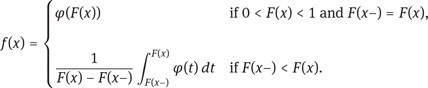
The lower bound is attained by X ∗ = f (φ), where f is a decreasing function on [0,∞) satisfying

The proof will use the following lemma, which yields another characterization of the relation ≽uni of second-order stochastic dominance.

Lemma 3.45. For two probability measures μ and ν on ℝ, the following conditions are equivalent:

(a) μ ≽uni ν.

(b) For all decreasing functions h : (0,1) → [0,∞),

where qμ and qν are quantile functions of μ and ν.

(c) The relation (3.30) holds for all bounded decreasing functions h : (0,1) → [0,∞).

Proof. The relation μ ≽uni ν is equivalent to

see Theorem 2.57. The implication (c)⇒(a) thus follows by taking h = (0 ,t] . For the proof of (a)⇒(b), we may assume without loss of generality that h is left-continuous. Then there exists a positive Radon measure η on (0, 1] such that h(t) = η([t, 1]). Fubini’s theorem yields

Proof of Theorem 3.44. Using the first Hardy–Littlewood inequality in Theorem A.28, we see that

where qX is a quantile function for X. Taking h(t) := qφ(1 − t) and using Lemma 3.45 thus yields (3.29).

Let us now turn to the identification of the optimal profile. Note that the function f defined in the assertion satisfies

where g is defined by g(t) = qX0(1 − t), and where Eλ[ · | qφ ] denotes the conditional expectation with respect to qφ under the Lebesgue measure λ on (0, 1); see Exercise 3.4.1 below. Let us show that X ∗ = f (φ) satisfies X ∗ ≽uni X0. Indeed, for any utility function u

where we have applied Lemma A.23 and Jensen’s inequality for conditional expectations. Moreover, X ∗ attains the lower bound in (3.29):

due to (3.31).

Remark 3.46. The solution X ∗ has the same expectation under P as X0. Indeed, (3.31) shows that

◊

Exercise 3.4.1. In this exercise we prove formula (3.31). Let (0, 1) be equipped with its Borel σ-algebra and the Lebesgue measure λ. Now let F : ℝ → [0, 1] be a distribution function, i.e., F is right-continuous, increasing, and satisfies limx↓−∞ F (x) = 0 and limx↑∞ F (x) = 1. Let q : (0,1) → ℝ be a quantile function for F. Show that for any measurable function φ : (0,1) → [0,∞) the conditional expectation Eλ[ φ | q ] is λ-a.s. given by

where the function f : ℝ → [0,∞] satisfies

To this end, argue in particular that f (q) is λ-a.s. independent of the values f (x) that are not specified by the above formula.

◊

Remark 3.47. The lower bound in (3.29) may be viewed as a “reservation price” for X0 in the following sense. Let X0 be a financial position, and let X be any class of financial positions such that X ∈ X is available at price π(X). For a given relation on X ∪ {X0},

is called the reservation price of X0 with respect to X , π, and .

If X is the space of constants with π(c) = c, and if the relation is of von Neumann-Morgenstern type with some utility function u, then πR(X0) reduces to the certainty equivalent of X0 with respect to u; see (2.11).

In the context of the optimization problem (3.21), where

the reservation price is given by E∗[ X∗ ], where X∗ is the utility maximizer in the budget set defined by w := E∗[ X0 ].

In the context of the financial market model of Chapter 1, we can take X as the space V of attainable claims with

and π(V) = · for V = · S. In this case, the reservation price πR(X0) coincides with the upper bound πsup(X0) of the arbitrage-free prices for X0; see Theorem 1.32.

◊

3.5Robust utility maximization

In this section we consider the optimal investment problem for an economic agent who, as in Section 2.5, is averse against both risk and Knightian uncertainty. Under the assumptions of Theorem 2.78 (b), the preferences of such an agent can be described by the following robust utility functional

where Q is a set of probability measures on (Ω,F) and u is a utility function. We assume that such a robust utility functional is given and that all measures in Q are absolutely continuous with respect to a fixed pricing measure P∗ on (Ω,F). We will also assume that all payoff profiles X are nonnegative and, for simplicity, that the utility function u is defined and finite on [0, ∞). As in Section 3.3, the budget set for a given initial capital w > 0 is defined as

The problem of robust utility maximization can thus be stated as follows,

In the sequel, we will assume that Q is a convex set, which can be done without loss of generality. Moreover, we will assume throughout this section that Q is equivalent to P∗ in the following sense: For all A ∈ F,

Clearly, our problem (3.33)would not be well-posed without the implication “⇒". Note that (3.34) implies that every measure Q ∈ Q is absolutely continuous with respect to P∗ but not necessarily equivalent to P∗.

If Q consists of the single element Q ≈ P∗, we have seen in Section 3.3 that the solution involves the Radon-Nikodym derivative dP∗/dQ. In our present situation, however, not every Q ∈ Q needs to be equivalent to P∗. The Radon-Nikodym derivative dP∗/dQ will therefore be understood in the sense of the Lebesgue decomposition; see Theorem A.17. With the convention for x > 0 it can be expressed as

It will turn out in Theorem 3.56 below that the following concept can be a key for solving problem (3.33).

Definition 3.48. A measure Q0 ∈ Q is called a least favorable measure with respect to P∗ if the density φ0 = dP∗/dQ0 satisfies

◊

Not every set Q is such that it admits a least-favorable measure with respect to a given measure P∗. But here are two examples in which least-favorable measures can be determined explicitly.

Example 3.49. Let Y be a measurable function on (Ω,F), and denote by μ its law under P∗. For ν ≈ μ given, let

The interpretation behind the set Q is that an investor has full knowledge about the pricing measure P∗ but is uncertain about the true distribution P of market prices and has only the “weak information” that a certain functional Y of the stock price has the distribution ν under P. Define Q0 as follows via its Radon-Nikodym derivative:

Then Q0 ∈ Q, and the law of φ0 := dP∗/dQ0 = dμ/dν(Y) is the same for all Q ∈ Q. Hence, Q0 is a least favorable measure.

◊

Example 3.50. For λ ∈ (0, 1) and a given probability measure P ≈ P∗ let

In Chapter 4, this set will play an important role as the maximal representing set for the risk measure AV@Rλ. If φ := dP∗/dP satisfies P[ φ > λ−1 ]> 0 and admits a continuous and strictly increasing distribution function Fφ(x) := P[ φ ≤ x ], then Qλ admits a least-favorable measure with respect to P∗, which is given by

where is the (unique) quantile function of φ and tλ is the unique solution of the equation

This will be proved in Corollary 8.28. In this case, one finds that

◊

Further examples for least-favorable measures can be found in Huber [158].

Remark 3.51. The existence of a least-favorable measure of a set Q with respect to P∗ is closely related to the concept of submodularity or strong additivity of the set function

which will be discussed in Sections 4.6 and 4.7. The Huber-Strassen theorem states that a set Q that is weakly compact with respect to a Polish topology on Ω admits a least favorable measure with respect to any other probability measure P∗ ≈ Q if and only if the set function c is submodular or strongly subadditive:

We refer to Huber and Strassen [159] and Lembcke [202]. Example 3.50 is a special case of this situation, since it will follow from Proposition 4.75 that the associated set function is strongly subadditive.

◊

Let us now show that we always have Q0 ≈ P∗ if Q satisfies a mild closure condition.

Lemma 3.52. Suppose that {dQ/dP∗ | Q ∈ Q} is closed in L1(P∗). Then every least favorable measure Q0 is equivalent to P∗.

Proof. Due to our assumption (3.34) and the closedness of {dQ/dP∗ | Q ∈ Q}, wemay apply the Halmos–Savage theorem in the form of Theorem 1.61 and obtain a measure Q1 ≈ P∗ in Q. We get

Hence, also P∗[ φ0 < ∞] = 1. That is, 1/φ0 = dQ0/dP∗ > 0 P∗-a.s., which is equivalent to Q0 ≈ P∗ by Corollary A.13.

We have the following characterization of least favorable measures.

Proposition 3.53. For a measure Q0 ∈ Q with Q0 ≈ P∗ and φ0 := dP∗/dQ0, the following conditions are equivalent.

(a) Q0 is a least favorable measure for P∗.

(b) If f : (0,∞] → ℝ is decreasing and infQ∈Q EQ[ f (φ0) ∧ 0 ] > −∞, then

(c) If g : (0,∞] → ℝ is increasing and supQ∈Q EQ[ g(φ0) ∨ 0 ] < ∞, then

(d) Q0 minimizes the g-divergence

among all Q ∈ Q whenever g : [0,∞) → ℝ is a continuous convex function such that Ig(Q|P∗) is finite for some Q ∈ Q.

Proof. (a)⇔(b): According to the definition, Q0 is a least favorable measure if and only if Q0[ φ0 ≤ t ]≤ Q[ φ0 ≤ t ] for all t ≥ 0 and each Q ∈ Q. By Theorem 2.68, this is equivalent to the fact that, for all Q ∈ Q, Q0 ◦ φ0−1 stochastically dominates Q ◦ φ0−1 in the sense of Definition 2.67. Hence, if f is bounded, then the equivalence of (a) and (b) follows from Theorem 2.68. If f is unbounded and infQ∈Q EQ[ f (φ0)∧0 ] > −∞, then assertion (b) holds for fN := (−N) ∨ f ∧ 0 where N ∈ ℕ. Thus, for all Q ∈ Q,

By sending N to infinity, it follows that EQ[ f (φ0)∧0 ]≥ EQ0 [ f (φ0)∧0 ] for every Q ∈ Q. After using a similar argument for 0 ∨ f (φ0), we get

(b)⇔(c) follows by taking f = −g.

(b)⇒(d): Clearly, Ig(Q|P∗) is well-defined and larger than g(1) for each Q P∗, due to Jensen’s inequality. Now take Q1 ∈ Q with Ig(Q1|P∗) < ∞, and denote by the right-hand derivative of g at x ≥ 0. Suppose first that is bounded. Since we have

where is a bounded decreasing function. Therefore, (b) implies that and so Q0 minimizes Ig( · |P∗) on Q.

To prove the assertion for convex functions g with unbounded gʹ+, let μQ denote the ∫ law of ∫ ∗under P. Then the preceding step of the proof implies in particular that (x − c)+ μQ(dx) ≥ (x − c)+ μQ0 (dx) for all c ∈ ℝ and each Q ∈ Q. Since in addition the result now follows from the equivalence (b)⇔(c) of Corollary 2.61.

(d)⇒(b): It is enough to prove (b) for continuous bounded decreasing functions f . For such a function f let Then g is convex. For Q1 ∈ Q we let Qt := tQ1 + (1 − t)Q0 and h(t) := Ig(Qt|P∗). The right-hand derivative of h satisfies and the proof is complete.

Remark 3.54. Let us discuss the connection between least-favorable measures and the statistical test theory for composite hypotheses, extending the standard Neyman-Pearson theory as outlined in Appendix A.4. In a composite hypothesis testing problem, one tests a hypothesis P against a null hypothesis Q and allows both P and Q to be sets of probability measures. Our situation here corresponds to the special case in which P consists of the single element P∗ and only the null hypothesis Q is composite. As in Remark A.36 one looks for a randomized statistical test ψ0 : Ω → [0, 1] that maximizes the power E∗[ ψ ] over all randomized tests ψ with a given significance level. For a composite null hypothesis Q, the significance of a randomized test ψ can be defined as supQ∈Q EQ[ ψ ]. Thus, the problem can be stated as follows:

where α ∈ (0, 1) is a given significance level and R denotes the class of all randomized tests (see Appendix A.4). This problem can be solved in a straightforward manner as soon as Q admits a least-favorable measure Q0 with respect to P∗. Indeed, choose κ ∈ [0, 1] and c > 0 such that

satisfies EQ0 [ ψ0 ] = α. Since ψ0 is an increasing function of φ0, Proposition 3.53 yields that

Moreover, if ψ is any other randomized test with supQ∈Q EQ[ ψ ] ≤ α, then in particular EQ0 [ ψ ]≤ α, and so Theorem A.35 implies E∗[ ψ ]≤ E∗[ ψ0 ], because ψ0 is an optimal randomized test for the standard problem of testing the hypothesis P∗ against the null hypothesis Q0. Therefore ψ0 is a solution of (3.35). Note also that the likelihood of a type 1 error for the test ψ0 is maximized by Q0. The fact that Q0 is independent of the significance level α is remarkable, and it explains why Q0 is called a ‘least-favorable’ measure.

◊

The next proposition prepares for the solution of the robust utility maximization problem (3.33).

Proposition 3.55. Let Q0 ≈ P∗ be a least favorable measure and φ0 = dP∗/dQ0.

(a) For any X ∈ B there exists a decreasing function f ≥ 0 such that f (φ0) ∈ B and

(b) Every solution X ∗ of (3.33) is of the form X ∗ = f ∗(φ0) for a deterministic decreasing function f ∗ : (0,∞) → [0,∞).

Proof. (a) Throughout the proof, we denote by qY (t) a quantile function of a random variable Y with respect to the probability measure Q0. Then we let F denote the distribution function of φ0 under Q0. As in Theorem 3.44, we consider a function f such that

Then f can be chosen as a decreasing function and satisfies f (qφ0) = Eλ[ h | qφ0 ],where λ is the Lebesgue measure and h(t) := qX(1 − t); see Exercise 3.4.1. Hence, Jensen’s inequality for conditional expectations and Lemma A.27 show that

where we have used Proposition 3.53 in the last step. Thus, f satisfies (3.36).

It remains to show that f (φ0) satisfies the capital constraint. To this end, we first use the lower Hardy–Littlewood inequality from Theorem A.28:

Here we may replace qX(1 − t) = h(t) by Eλ[ h | qφ0 ](t) = f (qφ0 (t)). We then get

Thus, f is as desired.

(b) Now suppose X ∗ solves (3.33). If X ∗ is not Q0-a.s. equal to a σ(φ0)-measurable random variable, then Y := EQ0 [ X∗ | φ0 ] must satisfy

due to the strict concavity of u. If we define as in (3.37) with Y replacing X, then the proof of part (a) yields that

and by (3.38) and (3.41),

in contradiction to the optimality of X ∗. Thus, X ∗ is necessarily σ(φ0)-measurable and can hence be written as a (not yet necessarily decreasing) function of φ0.

If we define f ∗ as in (3.37) with X ∗ replacing X, then f ∗(φ0) is the terminal wealth of yet another solution in B. Clearly, we must have E∗[ X∗ ] = w = E∗[ f ∗(φ0) ]. Thus, (3.39) and (3.40) yield that EQ0 [ φ0X∗ ] = ∫ 0 1 qφ0 (t) qX∗(1 − t) dt. But then the “only if” part of the lower Hardy–Littlewood inequality together with the σ(φ0)-measurability of X ∗ imply that X ∗ is a decreasing function of φ0.

We can now state and prove the main result of this section.

Theorem 3.56. Suppose that Q admits a least favorable measure Q0 ≈ P∗. Then the robust utility maximization problem (3.33) is equivalent to the standard utility maximization problem with respect to Q0, i.e., to (3.33) with Q replaced by {Q0}. More precisely, X ∗ ∈ B solves the robust problem (3.33) if and only if it solves the standard problem for Q0, and the values of the corresponding optimization problems are equal, whether there exists a solution or not:

for any initial capital w > 0.

Proof. Proposition 3.55 implies that in solving the robust utility maximization problem (3.33) we may restrict ourselves to strategies whose terminal wealth is a decreasing function of φ0. By Propositions 3.53, the robust utility of a such a terminal wealth is the same as the expected utility with respect to Q0. On the other hand, taking Q0 := {Q0} in Proposition 3.55 implies that the standard utility maximization problem for Q0 also requires only strategies whose terminal wealth is a decreasing function of φ0. Therefore, the two problems are equivalent, and Theorem 3.56 is proved.

Theorem 3.56 states in particular that the robust utility maximization problem (3.33) has a solution if and only if the standard problem for Q0 has a solution, and we refer to Theorem 3.39 (with W = +∞) for a sufficient condition.

Example 3.57. Consider the situation of Example 3.50, where for λ ∈ (0, 1) a least-favorable measure of Qλ with respect to P∗ is given by

Here φ = dP∗/dP satisfies P[ φ > λ−1 ] > 0 and admits a continuous and strictly increasing quantile function qφ with respect to P, and tλ is the solution of a certain nonlinear equation. Let us also assume for the sake of concreteness that is a HARA utility function with risk aversion γ ∈ (0, 1) and that E[ φ−γ/(1−γ) ] < ∞.

It was shown in Example 3.41 that the standard utility maximization problem under P has the solution

where φ = dP∗/dP. Note that X ∗ is large for small values of φ, that is, for low-price scenarios.

Now let us replace the single probability measure P by the entire set Qλ. By Theorem 3.56, the corresponding robust utility maximization problem will be solved by

where

It follows that

where r > 0 and c > 1 are certain constants. Thus, the effect of robustness is here that the optimal payoff profile X ∗ is cut off at a certain threshold. That is, one gives up the opportunity for very high profits in low-price scenarios in favor of enhanced returns in all other scenarios.

◊