Discounted Cash Flow

DCF valuation is a mainstay of M&A, and valuation in general, because it has several important advantages. DCF forces a consideration of the components that drive FCFs: revenues, operating costs, cash taxes, and investments in working capital and fixed assets (reflected in CAPEX)—investments that will support the projected growth of the merger. DCF is flexible and can easily accommodate changing assumptions as an acquirer thinks through scenarios of the future. The methodology also forces a consideration of the WACC, or the risk class of the assets under consideration.

DCF valuation is also, implicitly, a business plan—a story. It is your year-by-year belief of the growth and margins achievable for the businesses along with periodic investments that will be required to facilitate the strategic vision. You have to remember that your whole merger plan is based on promises—promises about future performance to stakeholders, including shareholders and employees. And if you don’t understand or haven’t thought through the business plan supporting those promises, then you will likely be challenged when it comes time to explain the logic of the deal.

Valuing a target using DCF essentially comprises two valuations: 1) the stand-alone value of the target—which means assessing the value of current business(es) plus the growth value of the business(es), like any value investor would; and 2) the amount and timing of the anticipated synergies—operating gains above stand-alone expectations—along with the one-time and ongoing costs to achieve those synergies. Thus, acquirers are building two business plans: the base case of the stand-alone value of the target and the overlay of all the net synergy benefits on top given the up-front investment of the premium.

When acquirers negotiate with targets, any upward or downward changes in price implicitly means assumptions about the inputs in the DCF model must be changing—a slightly lower WACC, a little bit more revenue growth in the fifth or sixth year, or a little bit lower investment in working capital to support the growth, and so on. That is all fine as long as those changes in assumptions are plausible.

“Multiples” approaches to valuing deals, such as enterprise value (EV)/EBITDA or EV/sales, are often viewed as more objective than DCF because they are based on the value of relevant comparables.² The DCF, in contrast, can be affected by “beauty is in the eye of the beholder” subjectivity. That said, any value based on an average market-based multiple implies a stream of cash flows that would have to discount back to that number. Of course, those approaches are subject to their own problems, like using the wrong multiple.

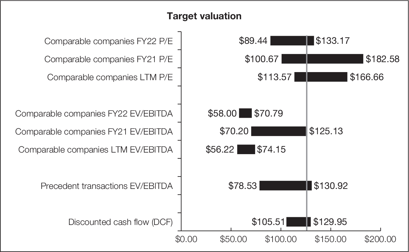
In practice, investment bankers follow a seemingly rigorous process and triangulate on value by looking at various EV or P/E multiples of comparable public companies (“compcos”), multiples for precedent or comparable acquisitions (“compaqs”), and the DCF. They then show a “football field” with a range of assumptions for each approach and determine the most “appropriate” range of values given by the three techniques. (See figure 4-1.)

But here’s the thing: The seller’s bankers are doing the same thing—except they don’t really care as much about the DCF valuation, although they’ll do one too. The seller and especially their board want a “fairness opinion” that shows they are realizing an appropriate or “fair” price for the company. Ultimately, they will want a premium that is based on how precedent transactions have been recently valued and how comparable companies, often at their 52-week highs, have been valued. Of course, that is the anchor for negotiations, because if they were to sell for less, directors of the seller will be sued for not getting a “fair” price.

FIGURE 4-1

Football field illustration

Thanks largely to the landmark 1985 case Smith v. Van Gorkom, which holds that officers and directors of a public company could be held personally liable for not making an informed decision about the appropriate selling price of a company, fairness opinions for sellers are practically mandated. In ruling against Van Gorkom and the directors of Trans Union, the Delaware Supreme Court found that, even though Trans Union shareholders would receive a 50 percent premium, the directors were grossly negligent because they did not properly inform themselves about the intrinsic value of the company. In what was a boon for investment banks, fairness opinions—and the market-based multiples of compcos and precedent transactions—effectively now largely determine what an acquirer will have to pay to do a deal.³

An Invitation for Mischief

Given the long-run disappointing evidence of the performance of major deals, often through overpaying, together with the well-accepted DCF approach to valuing deals, it begs the question of what has gone wrong. A plausible answer is that DCF is the perfect tool to support market-multiple approaches to value. In other words, DCF is an invitation for mischief and the perfect model for the tail—that is, what you have to pay—to wag the dog.

How? Because DCF valuation is seductively simple to use and incredibly sensitive to small changes in the variables in the model. Those changes can be pushed into an inflated terminal value at the end of the forecast period, especially for synergies. Not only that, but for a CEO dead set on doing a deal, it is so easy to bury optimistic assumptions about future revenue growth, margin sustainability, or investment requirements—and mix up synergies with already existing growth expectations—that only the most sophisticated analysts with a deep understanding of the businesses would be able to see where the bodies are buried. We’ve also learned that synergies pushed into later years lose their urgency and are easily forgotten.

For example, consider the following stream of FCFs with a 5 percent growth rate (table 4-1). For simplicity, we use a five-year model with a TV based on a “perpetuity with growth” or TV₅ = FCF₆/(c − g), where c is the cost of capital and g is the projected growth rate of the FCFs. We show a range of costs of capital and c − g spreads that can drive a wide range of valuations. At a 7 percent cost of capital, for example, just nudging the perpetual growth rate from 2 percent to 3 percent (or a c − g spread from 0.05 to 0.04) yields a valuation of $2,861.3M, up from $2,383.6M, for an increase of 20 percent, which might be used to justify a higher premium.

Of course, it is difficult to make forecasts five or 10 years into the future; projections by their nature are risky, and that is where the pitfalls lie. Common red flags are when an acquirer inserts unrealistic operating margin improvements or understates CAPEX to support all the wonderful new revenue growth that will result from the strategy of a deal. That often shows up in the model as significant increases in earnings before interest and taxes (EBIT) without the required investments. The result: a much higher valuation because FCF is overstated forever in perpetuity, buried in an inflated terminal value. That is how easy it is for the tail to wag the dog.

In the M&A context, markets have already done a valuation of the target, and your company, for that matter. So, the trouble often stems from the acquirer’s assumptions about operating gains over already existing growth expectations—the synergies. Your banker will tell you the premium that will be required to do the deal, and so even the most prepared acquirers must be cautious of plugging numbers into a model. At the end of day, the premium you pay signs you up for a future business case. If you pay—that is, invest—all that luxurious capital up front and don’t deliver on that business case, you will have let down your shareholders and your employees.

That is exactly why DCF can be an invitation for mischief—because it is so easy and seductively simple to bury assumptions that drive wild swings in “value” and support virtually any price required to please the seller and get the deal done. At the minimum, acquirers should not mix up synergy assumptions with the value and growth expectations of the stand-alone business of the target—or of the acquirer. That is a real invitation for mischief and the resulting predictable overpayment.

Now, we are not saying not to use DCF—far from it. DCF is widely accepted and theoretically correct and yields the most you should be willing to pay for an asset to yield a cost-of-capital return on that investment. Used properly and with realistic discipline about the prospects for the target under your ownership, DCF is an effective way of valuing assets so that you don’t overpay for a series of free cash flows over a specific forecast period. DCF is at its core a business plan that shows how much cash is available to investors after making required investments in working capital and fixed assets to drive the growth plans.

Here’s the crux of the matter: When you are building a DCF valuation model, the numbers you put in the model are assumptions, but when you buy the company those numbers become promises.

There is another way, an equivalent mirror image of DCF, if you will, of showing what you are indeed promising when you pay a given amount for an acquisition—a simple way of converting a value given by a discounted series of free cash flows to an equivalent series of periodic benefits relative to the cost of capital each period. We want a way to take that value (or a range of values) from a DCF, cut through the clutter of all assumptions, and recast that value into a stream of yearly performance increases that are measurable and trackable, and reflect the promises an acquirer is making by doing a deal at a given price.

What Are You Promising?

As Warren Buffett once famously wrote about M&A, “Investors can always buy toads at the going price for toads. If investors instead bankroll princesses who wish to pay double for the right to kiss the toad, those kisses better pack some real dynamite.” His point is so clear: Since investors can diversify on their own, without paying a premium, synergies must be thought of as improvements as a result of the merger—“if but for the deal.” Paying a premium only raises the operating performance bar (perhaps Mr. Buffett said it better). This is as true for the acquisitions of private companies or carve-outs of divisions as it is for public targets, except that acquirers won’t have a public market valuation (they’ll have to do that themselves).⁴

Thus, operating gains over stand-alone expectations—the synergies—must be performance improvements over what was already expected. Illuminating synergy expectations in addition to already existing expectations requires an approach that separates value into its known and expectational components. The result is a forward-looking view of just how much the bar is being raised. That approach should be able to dissect the total value of a company into the value of the current business without improvements, the current expectations of improvements in the stand-alone businesses, and the additional improvements required to fully justify the price, and the premium, you are about to pay.

Although DCF accommodates a business plan, even when done with discipline—and in deals, with a full understanding of how the integration of the target will yield benefits—it suffers an important shortcoming especially for deals: the major input, the FCFs, do not provide a reliable measure of periodic economic operating performance. That’s because, by definition, FCF subtracts the entire cost of an investment in the year in which it occurs rather than spreading the cost of the investment over the life of the asset that has been acquired with a capital charge. In other words, DCF, and FCFs specifically, don’t offer an obvious lens to express whether acquirers are creating economic value each period with the capital they are committing or have committed to a deal.

That shortcoming of FCF as a measure of periodic value creation can be avoided by using the concept of EVA. EVA is calculated as NOPAT minus a capital charge equal to invested capital for the period times the WACC. (See the sidebar, “Calculation of Economic Value Added.”) Unlike FCF, EVA effectively capitalizes instead of expensing much corporate investment, and then holds management accountable for that capital by assigning the capital charge we just described. EVA is based on the idea of economic profit where value is created when a company covers not only its operating costs but also the cost of capital—the return expected by investors.⁵

Fortunately, EVA offers a different but equivalent lens for FCF because the present value of the cost of a new investment is the same for EVA and FCF. The present value of the deprecation expense and capital charge for EVA is exactly equal to the initial investment cost for FCF. The present value of future FCF is equal to the present value of future EVA plus beginning capital. (We need to add back beginning capital to recover the EVA charge on beginning capital—a charge that does not affect FCF.) Recasting market value based on the idea of EVA as economic profit, or the value created by invested capital, can be summarized as follows:

Market Value = Invested Capital + Present Value of Future EVAs

EVA is especially useful for performance measurement and evaluation because it allows us to dissect a company’s market value into its known and expectational components. We can do this by breaking the present value of all future EVAs into two pieces: 1) the present value of maintaining the company’s current EVA (its perpetuity value), which we know; and 2) the present value of the expected EVA improvements above current EVA—that are maintained.

Don’t worry, we’re not introducing some crazy new idea of valuation. In fact, both of these approaches—DCF and EVA—were developed and proved equivalent in the same famous 1961 Journal of Business article “Dividend Policy, Growth, and the Valuation of Shares,” by Nobel Prize winners Franco Modigliani and Merton Miller. Modigliani and Miller—affectionately known as M&M—were giants in academic finance, and their famous Equations 11 and 12 are well studied by students of finance. Equation 11 is the DCF model and Equation 12 is what they termed the “investment opportunities approach” (IOA), which laid the groundwork for the EVA approach. In fact, M&M thought this approach was the most natural from the standpoint of an investor considering an acquisition because it offers a view of value based on whether the return on new investments would exceed their cost of capital (see appendix B).⁶

M&M’s Equation 12 yields a practical expression in the context of EVA. Incorporating beginning capital and both components of EVA (NOPAT and the capital charge) into M&M’s IOA equation implies the following fundamental EVA equation, which breaks total market value into its known and expectational components.⁷ (For additional details on the EVA equation, see appendix C.)

Where Market Value₀ is a company’s total market value today (equity plus debt); Cap₀ is beginning book capital (or total assets minus non-interest bearing current liabilities); c is the required cost-of-capital return, or the WACC; EVA₀ is beginning EVA (NOPAT₀ − Cap−₁ × c) or prior year’s NOPAT minus the prior year’s capital charge; and ΔEVA_t is investors’ expectation, today, of EVA improvement in year t. Notice that is exactly where we started the discussion, except we have broken market value into what we can measure today and the expectations of improvements in the future.

The sum of the first two terms, beginning capital and the present value of constant current EVA (capitalized current EVA, its perpetuity value), can be thought of as “current operations value” (COV). The remainder of the expression, the third term, can be thought of as “future growth value” (FGV). We express FGV as the capitalized present value of expected annual EVA improvements—improvements that will yield a cost-of-capital return on the growth value investors are awarding the company today. We capitalize the present value of expected improvements because we assume that each improvement is maintained in perpetuity. Restating our earlier market value expression, we now have:

Market Value = Beginning Invested Capital + Capitalized Current EVA + Capitalized Present Value of Future EVA Improvements

So, market value today can be expressed as performance we know today and improvements expected in the future, or

Market Value = Current Operations Value + Future Growth Value

Since investors expect a cost-of-capital return on the total market value of a company, then they expect a cost-of-capital return on COV and a cost-of-capital return on FGV because they are buying both. Merely maintaining current economic performance, or current EVA, and offering no EVA improvements, will only deliver enough NOPAT to provide a cost-of-capital return on COV but no return at all on FGV. The bottom line: FGV implies investors expect improvements in EVA.

For example, let’s say you are buying a company with a market value of $2B with beginning invested capital of $1B, a recurring stream of NOPAT of $120M, and a 10 percent WACC and current EVA of $20M. For simplicity, we assume no changes in capital from the prior year. We have:

$2B = Cap0 + Capitalized Current EVA0 + Capitalized Present Value of Future EVA Improvements

$2B = $1B + $20M/0.1 + $800M

$2B = $1.2B + $800M

In this example, our COV is $1.2B and FGV is $800M. Maintaining current EVA of $20M ($120M − capital charge of $100M) will only deliver enough NOPAT to yield a cost-of-capital return on COV.⁸ The company will need to generate EVA improvements (ΔEVA) sufficient to justify the $800M of FGV it is currently being awarded by the market. There are many ways to achieve that value.

For example, at the extreme, if you could deliver increased performance of $80M of EVA improvement in the current year, perhaps through a major cost reduction effort, and maintain that forever, then you could certainly justify growth value beyond the value of current operations today. From our EVA equation above, and using a simplified notation, we have:

FGV is the third term of the market value equation:

With a one-time improvement, the FGV expression would reduce to:

So, with FGV of $800M and WACC of 10 percent, required ΔEVA₁ for the one-time improvement will be:

ΔEVA1 = 0.1 ($800M) = $80M or,

$800M = 11 ($80M/1.1) or a spike of $80M of ΔEVA that is maintained

That one-time change would represent a huge increase in performance, which is probably unrealistic in one year. While that would be an extraordinary accomplishment, if EVA weren’t expected to grow from there, you would have effectively converted FGV to COV (it becomes next period’s current EVA), and you would have become a no-growth company, from a value perspective. Of course, if that level of performance increase was a signal of a bright future, then investors would surely bid up the price of your shares, awarding you with significant growth value.

Now, let’s take the FGV portion of above and assume that instead of a one-time increase in EVA, you could achieve a stream of equal annual EVA improvements, in perpetuity, which when capitalized is equivalent to the one-time spike. Here, we’ll assume that FGV remains constant. Using our FGV expression:

With equal annual EVA improvements in perpetuity, the FGV expression reduces to:

Using FGV of $800M and WACC of 10 percent from our example, required perpetual annual ΔEVA will be:

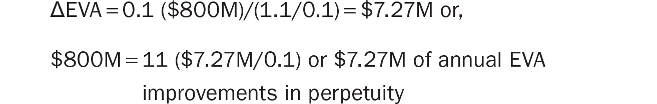
So, equal annual EVA improvements of $7.27M in perpetuity would equate to a 10 percent WACC return on $800M in FGV.⁹ If growth expectations remain the same, we would have constant FGV of $800M and COV would increase each period as would the market value. The major takeaway is that when investors are expecting valuable growth, they are willing to pay for FGV. However, if you don’t deliver or can’t maintain those expectations, your share price will suffer accordingly.

What Happens When You Pay a Premium?

What happens when you offer to pay a premium for our target company? Let’s say a 40 percent premium, or $800M for our $2B company. What have you done? You have added, immediately, $800M, directly to the FGV of the target, which was already $800M, for a new grand total of $1.6B in FGV.

We started with $2B = $1.2B + $800M, but with your offer of a 40 percent premium, we now have:

$2.8B = $1.2B + $800M + $800M

The target still has $1.2B of COV but you have doubled FGV. Are you starting to get the picture?

That is what you are setting up for investors when you pay a premium. Paying a premium establishes a brand-new business performance problem that never existed, and no one ever expected. In the example above, you are essentially doubling the required improvements in performance to earn a cost-of-capital return on FGV from the total investment. In this simple example, for either of our ΔEVA approaches above the required ΔEVA will double.

Once you acquire the target with the $800M premium, you have fixed the price of the target. The target’s value won’t fluctuate in value anymore. The only share price that will fluctuate is yours—based on the expected return you can generate with all that luxurious new capital. You will need an additional cost-of-capital return, just to break even. Failing to demonstrate a path to do that will likely lead shareholders—and other stakeholders—to question and perhaps doubt the logic of the deal and the offer price, right from announcement. Merely achieving expected stand-alone improvements, a cost-of-capital return on current FGV, but not realizing sufficient synergies on top of that is a recipe for trouble.

Because the offer of a premium is a surprise to investors (and a pleasant surprise to the sellers), equal annual improvements over time in perpetuity are likely not going to be very satisfying and will probably try their patience. Even if you have a long track record, a significant premium for performance not expected before is still a shock. And just telling investors you will double what they expected before won’t work. The good news: Our EVA equation handles that with ease.

Let’s focus on the $800M premium and consider a ΔEVA ramp up of required synergies. From our FGV expression:

So, a three-year ramp up starting in year 1 would mean:

Where one solution in this case with a three-year ramp up would be:

$800M = 11 [($20M/1.1) + ($30M/1.21) + ($39.6M/1.33)]

In other words, an increase of $20M in the first year, an additional $30M increase in the second year, and additional $39.6M increase over that in the third year—so we have a run rate of EVA improvements over current EVA of roughly $90M per year by the end of year 3 that is maintained. There are lots of combinations you could offer, but the sooner the better.

You might recognize this as the familiar synergy ramp up typically observed in successful deal communications. Imagine what happens when you don’t offer an aggressive plan to deliver synergies. A ramp up effectively shows a path to justifying or “paying off” the premium. Once the full run rate is achieved after year 3, you will have converted that FGV from the premium into COV. Presumably, investors will take that confidence as a signal that there will be ongoing profitable growth as a result of the many long-term strategic benefits of the deal and be willing to pay for additional growth value—that is, that the “synergies” will continue to grow.

If we assume that your company (or another acquirer) has stand-alone required ΔEVA in perpetuity of $10M, we get the schedule shown in table 4-2, which illustrates the EVA improvements required for the stand-alone companies along with a three-year ΔEVA ramp up needed to justify the $800M premium, for the next five years (and beyond).

The increase in FGV and implied increase in ΔEVA in this example translates to huge percentage increases in required performance. If investors believe that such gains aren’t possible, then your share price will fall right on Announcement Day, to adjust for the proper growth value. On the other hand, if you project a confident story with numbers they can follow, and the deal is really strategic, you will likely be rewarded with additional growth value, and a higher share price, as is the case with successful acquisitions. (We address investor communications in chapter 5.)

Thus far, we have developed something important and useful: a rapid and valid method of taking the premium “justified” by the DCF or any other valuation technique and translating it to a sensible ramp up of synergies—ΔEVAs—that will offer a cost-of-capital return on the premium. It is a sanity check that you understand what you are promising based on your valuation.

On that note, let’s revisit what ΔEVA means in the context of synergies to make this tangible. Since ΔEVA must be Δ(NOPAT − Cap × c) or (ΔNOPAT − ΔCap × c), if we assume for simplicity there aren’t any significant increases in invested capital post deal, then that reduces to changes in NOPAT—which could be compared to the NOPAT assumptions in the original DCF valuation. That said, any additional capital investments and any additions to the premium, such as one-time cost to achieve synergies, will require commensurate improvements in NOPAT.

Now, suppose you tell your investors there might be a delay in getting a cost-of-capital return on the new growth value—the premium—you have just created by giving the target’s shareholders their windfall. How might your investors respond?

Delay: What Do Investors Hear?

Remember from chapter 1 when you wanted to buy that apartment in New York City? Well, you go through with it, but you need a mortgage to pay the entire value that includes that 50 percent premium ($500,000) you are paying over market value. So, you agree to pay $300,000 as a down payment and approach your local bank and go through the necessary paperwork to secure your $1.2M loan. You feel ambitious so you take a 10-year mortgage with a 5 percent interest rate on the loan. For the bank to earn its 5 percent for the life of the loan you will need to pay $12,728 per month for 10 years. Now, imagine, you are at the closing and there are many new people around the table—the sellers, the lawyers, the brokers on both sides, and of course your banker.

Now, just before you sign on the dotted line, you lean over to your banker and tell them, “Uhm, I may miss a few payments,” just before you sign the loan agreement.

“What?” asks your banker.

“Yeah,” you say in return. “And not only that, I don’t know exactly when I’m going to start paying. The only thing I know for sure is that I’m going to miss a fair number of payments.”

“Oh, boy,” mumbles your banker. “How many payments do you think you might miss?”

And you reply, “It could be 24 or even 36 months,” you say, but add emphatically, “Trust me, I’m good for it.”

That is what paying a premium sounds like to investors, when you tell them you are going to pay more than anyone else in the world is willing to pay for a company and you are not going to realize a return on all that new capital—the synergies—until some vague time in the future. You are taking out a mortgage for your shareholders that they didn’t need to buy shares of the target on their own, and they will expect you to get a return on all that new capital. You can expect investors to be suspicious if you can’t communicate a sensible plan, or if you signal you have none. That’s the recipe for a typical negative market reaction. Offering a premium means you will need to show significant improvements early on, or your market value will decline to reflect the appropriate FGV.

Putting It All Together: Homeland Technologies Makes an Offer for Affurr Industries

Chas Ferguson—the CEO of Homeland Technologies, whom we introduced in chapter 2—proceeded with his quest for potential deals that might rapidly increase the size of Homeland and build shareholder value in the process. His bankers brought him several deals and he focused on Affurr Industries, for which he performed FDD, CDD, and ODD, and Affurr Industries seemed like a perfect fit—at a 40 percent premium.

When you buy another company, you don’t just pay a premium, you also immediately write up the invested capital of the target to the total market value, and we have to account for that. In other words, when you buy a company at the premium, you need to generate a cost-of-capital return on the COV and FGV of the target (because you have written up the capital on the combined balance sheet when you pay full market value of the target’s shares and assume the debt) plus a cost-of-capital return on the premium.

To do that we can look at both acquirer and target as stand-alone companies, and then put them together as a new company, with a new amount of invested capital, a new WACC for the combined company, and a new COV and FGV. We can then show the required EVA improvements for each company pre-acquisition and how those required EVA improvements change as a result of the deal. For simplicity, we assume the new WACC is a weighted average, based on market values, of the pre-deal WACCs of both companies.¹⁰

First, for both the acquirer and target, begin with total market value (equity market cap plus debt). Then determine the beginning invested capital (total assets minus non-interest-bearing current liabilities (NIBCLs)) for each company. Next calculate current EVA (prior year NOPAT − (prior year beginning capital × WACC)) and capitalize current EVA at the respective WACC. Per our EVA equation, adding beginning capital plus capitalized current EVA yields COV. Finally, total market value minus COV gives us FGV—the capitalized present value of future EVA improvements expected by investors.¹¹

Let’s examine Homeland and Affurr Industries as two independent companies and take this step by step, starting with the fact sheet in table 4-3 (values in $M).

Let’s look at each company separately so we can determine what investors are expecting from each company as a stand-alone. Table 4-4 relates to Homeland Technologies, where Current EVA = NOPAT − Capital Charge, or 390 − (2000 × 0.1) = $190M. We have FGV of $1,100M so our perpetual ΔEVA = (1,100 × c)/((1 + c)/c), or 1,100(0.1)/11 = Δ$10M every year.

Table 4-5 relates to Affurr Industries, where current EVA = NOPAT − Capital Charge, or 120 − (1,000 × 0.1) = $20M. We have FGV of $800M so our perpetual ΔEVA = (800 × c)/((1 + c)/c), or 800(0.1)/11 = Δ$7.27M, just like we showed earlier.

Now for what you’ve all been waiting for: putting the two companies together in six easy steps:

1. Calculate total market value of combined entity:   Pre-Announcement Market Value of Buyer + Pre-Announcement Market Value of Target + Premium
2. Capital of combined entity:  Beginning Capital of Acquirer + Market Value of Target + Premium
3. Calculate new capitalized current EVA:  [Combined Prior Year NOPAT − ((Prior Year Beginning Invested Capital of Acquirer + Market Value of Target + Premium) × New WACC)] / New WACC
4. Calculate new COV:  Capital of Combined Entity + New Capitalized Current EVA
5. Calculate new FGV:  Total Market Value of Combined Entity − New COV
6. Calculate required EVA improvement:  (New FGV × New WACC) / ((1 + New WACC)/New WACC)

Step 3 is important. We are restating current EVA as if the acquirer had all the new capital—the total investment in the target and the target’s debt—on its balance sheet before the deal announcement (i.e., our pro-forma base year). That is why we add the acquirer’s prior year beginning capital plus the total market value of the target plus the premium to calculate the capital charge for current EVA—effectively the new starting point we use to restate FGV and the improvements required in the future. Our method allows an easy comparison of the stand-alone ΔEVA expectations before the deal with the combined required changes as a result of the deal.¹²

Table 4-6 puts the two companies together without the premium.

Let’s walk through the calculations:

1.  New Market Value = 5,000 + 2,000 = 7,000

2.  New Capital = 2,000 + 2,000 (because you’ve written up the target’s capital to market value)

3a.  New NOPAT = 390 + 120 = 510

3b.  New Capital Charge = (2,000 + 2,000) × 0.1 = 400

3c.  New Current EVA = NOPAT − Capital Charge = 510 − 400 = 110

3d.  New Capitalized Current EVA = 110/0.1 = 1,100

4.  New COV = 4,000 + 1,100 = 5100

5.  New FGV = 7,000 − 5,100 = 1,900

6.  New ΔEVA = 1,900 (0.1)/11 = Δ$17.27M every year in perpetuity

You’ll notice a few things that illustrate the mechanics: We now have lower capitalized current EVA, but we have more invested capital because Homeland bought the target at its market value; the new COV is just the sum of the independent COVs. So the new FGV is also the sum of the independent FGVs, and the total required EVA improvements remain the same.¹³

Table 4-7 adds the 40 percent premium of $800M, and voilà!

Let’s again walk through the calculations:

1.  New Market Value = 5,000 + 2,800 = 7,800 (adding the premium)

2.  New Capital = 2,000 + 2,800 (because you’ve written up the target’s capital to market value plus the premium)

3a.  New NOPAT = 390 + 120 = 510

3b.  New Capital Charge = (2,000 + 2,800) × 0.1 = 480

3c.  New Current EVA = NOPAT − Capital Charge = 510 − 480 = 30

3d.  New Capitalized Current EVA = 30/0.1 = 300

4.  New COV = 4,800 + 300 = 5,100

5.  New FGV = 7,800 − 5,100 = 2,700

6.  New ΔEVA = 2,700 (0.1)/11 = Δ$24.54M every year in perpetuity¹⁴

New Homeland’s combined COV is still the same and FGV has increased by the amount of the premium. Like before, we have lower capitalized current EVA, but we have more capital, and the premium is simply a direct addition to combined FGV.

The new ΔEVA of $24.54M increases by the amount of the premium $800M times its required cost-of-capital return on the premium ($800M × (0.1)) divided by ((1 + c)/c) (or 11), which yields a perpetual annual increase of $7.27M over the independent stand-alone expectations of both companies.

Here’s the big thing: Although this is a simplified example, taking the dollar premium times c/((1 + c)/c), where c is the WACC, gives us a rapid calculation of required ΔEVA with equal annual improvements in perpetuity. We can of course convert that to a ramp up that will be more satisfying to investors, as we showed in the earlier schedule (see table 4-2). And investors can also do that in seconds.

A few important notes: As we discussed earlier, these are expected increases in EVA (NOPAT minus the capital charge), so if there aren’t major additions to capital, then we are talking about changes in NOPAT. Because NOPAT is by definition after-tax, we would need to gross up that number to the pre-tax synergy number (given an effective tax rate), which is improvement in EBIT we would typically offer at announcement. NOPAT changes can take the form of faster growth or better profitability. And we could easily develop a table of different growth or profitability improvements that would yield the required result. Finally, because DCF and EVA are equivalent, we can compare the EBIT or NOPAT changes from our approach against the NOPAT changes in the DCF.

Revisiting Our Mega-Deal: Future Industries Makes an Offer for Cabbãge Corp

Now let’s work through the mega-deal example we introduced at the beginning of the chapter. We can now disclose that Future Industries, a large and rapidly growing technology player, made an offer for Cabbãge Corp, a large company that has developed innovative applications at the intersection of technology and healthcare. Table 4-8 shows the fact sheet.

Consistent with our approach for Homeland and Affurr, let’s look at each company separately so we can understand investor expectations for each company as stand-alone enterprises.¹⁵ (See table 4-9 for Future Industries and table 4-10 for Cabbãge Corp.)

Now, we follow our method and combine the two companies to form the new Future Industries, along with the $10B premium Future is offering for Cabbãge Corp. We also calculate the new WACC based on the market values of both companies plus the premium, which is 7.77 percent.¹⁶ Table 4-11 shows the COV, FGV, and perpetual annual EVA improvements required to justify the FGV of the new Future Industries and Cabbãge Corp combination.

Let’s again walk through the six steps of calculations:

1.  New Market Value = 40,924.41 + 45,799.24 + 10,000 = 96,723.65 (adding the premium)

2.  New Capital = 33,598.36 + 45,799.24 + 10,000 = 89,397.60 (because you’ve written up the target’s capital to market value plus the premium)

3a.  New NOPAT = 1,889.34 + 3,151.33 = 5,040.67

3b.  New Capital Charge = (32,009.84 + 45,799.24 + 10,000) × 0.0777 = 6,822.77

3c.  New Current EVA = NOPAT − Capital Charge = 5,040.67 − 6,822.77 = −1,782.10

3d.  New Capitalized Current EVA = −1,782.10/0.0777 = −22,935.65

4.  New COV = 89,397.60 + −22,935.65 = 66,461.95

5.  New FGV = 96,723.65 − 66,461.95 = 30,261.70

6.  New ΔEVA = 30,261.70 (0.0777)/(1.0777/0.0777) = Δ$169.53M every year in perpetuity

We can now easily compare the combined pre-deal stand-alone annual EVA improvement expectations of both companies with the new expectations for annual improvements, given that Future is paying the full market value for the shares of Cabbãge (and assuming the debt) plus a $10B premium. Table 4-12 shows that Future is promising a perpetual increase in annual EVA improvements of $57.42M, or a whopping increase of over 50 percent every year in perpetuity. We also show an easy approximation to our method by just taking the $10B premium on its own as a direct increase in FGV and calculating the perpetual annual increase in EVA improvements, using our new WACC, and our formula for perpetual ΔEVA.¹⁷

Let’s pause for a moment, because this is very important and the crux our journey. If we just directly take the $10B premium as new FGV and multiply by c/((1 + c)/c), we arrive at $56.02M of required perpetual annual EVA improvements, which is very close to working through the whole method.¹⁸

In other words, performing a sanity check for any DCF or multiples-based valuation is simple to do.

Now, making this more realistic for what you will need to announce, we can convert perpetual equal annual improvements and show a three-year ramp up of required synergies expressed as EVA improvements. We are essentially converting that FGV into COV by the end of the three years, which is likely far more satisfying for investors. And remember, because EVA is based on NOPAT, these are after-tax results. Recall our formula earlier in the chapter for a three-year ramp up:

Using the $10B premium as FGV at a 7.77 percent WACC with an illustrative 25 percent, 35 percent, and 40 percent path to value, and a level P&L run rate after three years, gives us the figures in table 4-13.

Because these are EVA improvements, without significant additions of capital, they are changes in NOPAT.¹⁹ That would translate to an after-tax P&L impact of $194M in the first year, $487M ($194M + $293M) in the second year, and a level run rate of $848M ($194M + $293M + $361M) in the third year maintained going forward.²⁰

However, if the new Future Industries were to delay realizing synergies until the third year (with no synergies realized in the first two years), this would blow up to $902M in after-tax improvements required all in the third year and maintained—not even close to the $361M increase of after-tax synergies required after three years, with a reasonable ramp up. You might also notice that the $902M in after-tax synergies is not even close to the $500M in pre-tax synergies (or $360M after tax with a 28% effective tax rate) that Future announced at the beginning of the chapter, with no timetable for delivery. When you don’t offer a timetable, investors don’t know what to think other than you don’t have a plan. Little wonder our buyer lost the majority of the premium right on Announcement Day.²¹

The big finale is—wait for it—anybody can do these calculations before making an offer. If the results are not consistent with the after-tax, or equivalent pre-tax synergies you are about to promise the markets, “Houston, you may have a problem.”

Conclusion

The math is clear, but let’s reiterate the chapter’s main points. Paying a premium for an acquisition requires a business plan to support the up-front investment. DCF valuation—although widely used—is sensitive to small changes buried in future assumptions, especially for synergies, and presents the potential for the tail to wag the dog to justify the price and premium you have to pay to get the deal done. Notably, DCF assumptions pre-announcement become promises embedded in the offer price of the deal—the acquirer is on the hook to achieve them. Once you fix the price of the target and pay for the deal, the only price that will fluctuate is yours, not the target’s.²²

Any delay in achieving those improvements will prove costly. Investors don’t like it when you tell them you can’t pay the “mortgage” for a while. Investors are smart: They know you can’t just flip a switch and turn on synergies some time in the future. As a consequence, any deal must include some ramp up of synergies at announcement that does two things: 1) gives investors confidence you have a plan, and 2) yields a cost-of-capital return on the premium paid.

Future growth value, or FGV, implies EVA improvements, and any premium paid only raises the bar. Translating the premium to a ramp up of EVA and NOPAT improvements is a sanity check of the output of a DCF valuation that justifies a premium—and investors can do that calculation in seconds. Assuming no significant increase or decrease in invested capital, and the associated capital charge, EVA changes become changes in NOPAT—but, of course, any increases in invested capital will require a commensurate increase in NOPAT to compensate for the additional capital charge.

Remember, this process is not only a test of the valuation of the target; it’s implicitly a review of the business plan of the deal—a story to be told to the board, to employees, and to investors. If expectations aren’t met, the acquirer’s stock price will drop. Announcement Day, the subject of the next chapter, is the day when all of these elements come together, and must be treated as seriously as every other part of the M&A process.