In chapter 4, we defined current market value (MV₀) as beginning capital plus the present value of future EVAs. Many will recognize this as consistent with the popular MVA (market value added) concept where the MVA of a firm is its market value less invested capital. We have:

MV0 = Invested Capital + Present Value of Future EVAs

We broke future EVAs into two parts: maintaining current EVA and achieving EVA improvements (ΔEVAs). We employed the following expression for current total market value based on beginning invested capital, capitalized current EVA, and the capitalized present value of expected EVA improvements:

We referred to the sum of the first two terms as “current operations value” (COV) and the third term as “future growth value” (FGV). Investors expect a cost-of-capital return (c), the WACC, on both COV and FGV. Merely maintaining current EVA (EVA₀) will yield a cost-of-capital return on COV but no return at all on FGV. Thus, justifying FGV will require EVA improvements.

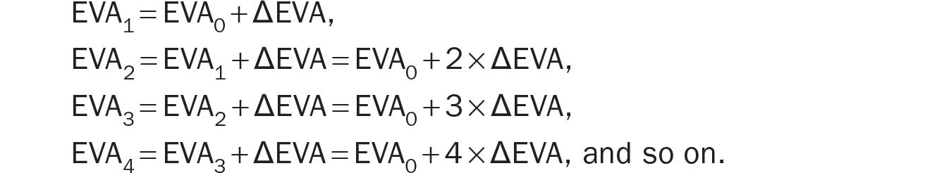
Although the EVA equation for market value is a straightforward adaptation of M&M’s equation 12 (reviewed in appendix B), it is useful to develop the intuition of the EVA equation.¹ Let’s say that a firm has EVA of EVA₀ today, which is expected to change by ΔEVA in the first period. What does that mean? It means that this period’s ending EVA (i.e., next period’s beginning EVA) is EVA₁ = EVA₀ + ΔEVA.

If we assume constant FGV and define ΔEVA as an equal annual improvement and each change persists in perpetuity, EVA in each period should be higher by ΔEVA of the previous period. So,

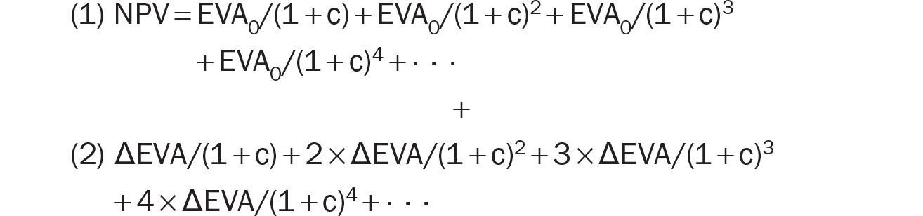
In EVA terms, the net present value (NPV) of a business is the present value of its per-period EVAs (the present value of future EVAs) because we take a capital charge for investments. Using that concept, we have:

Expanding EVA₁, EVA₂, EVA₃, and so on gives us following:

We can separate all the EVA₀ terms from the ΔEVA terms and group the EVA₀ terms together. We do the same for the ΔEVA terms. This creates two series from the equation:

The first series represents the present value of a perpetuity of EVA₀ dollars starting its payoff at the end of the first period (where today is time zero). Thus, its value will converge to EVA₀/c, the present value of a level perpetuity. So, we now have:

The second series involving ΔEVA is also quite intuitive once it is simplified and broken down into its components.

Let’s rewrite the second series (the series of ΔEVA) in an intuitive way that helps us get a closed-form expression:

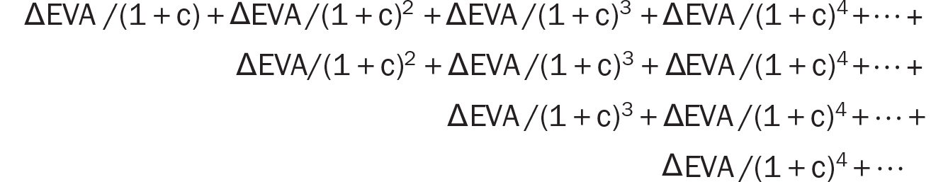
You will notice that this new rewritten series is identical to the previous ΔEVA series. However, it is easier to solve. Notice the first row of the above series: it represents the present value of a perpetuity of ΔEVA dollars starting its payoff at the end of the first period. Similarly, the second row represents a perpetuity of ΔEVA dollars starting its payoff at the end of the second period, and so on.

We already know the closed forms for these kinds of perpetuities. The present value of a $1 perpetuity starting its payoff at the end of the first period is $1/c. The present value of a $1 perpetuity starting at the end of the second period is ($1/c)/(1 + c), which is exactly the same perpetuity value as the previous perpetuity but with an extra period of discounting to account for the one-period delay in beginning its payoff. Similarly, the present value of a $1 perpetuity starting at the end of the third period is ($1/c)/(1 + c)², and so on.

Substituting these values, we get a simplified second series:

Now, we need one more step to get a simplified expression for this series. Since we’ve assumed that the ΔEVAs are equal annual improvements, then, excluding the first term, we see that the second term and onwards represents a perpetuity of ΔEVA perpetuities starting at the end of the second period. Thus, its present value will be (ΔEVA/c)/c.

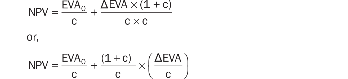
So, the total value of this series becomes:

We combine this expression for the second series (the ΔEVA series) with the expression for the first series (the EVA₀ series) to arrive at a simplified formula that describes the NPV of a business in terms of its current EVA and expected future annual EVA improvements.

Relaxing the assumption of constant FGV and allowing for different EVA changes in each year t yields the second and third components of our EVA equation for market value:

So, for example, if each ΔEVA_t is $100 in perpetuity, and with constant FGV, then would simply reduce to or .

Adding beginning invested capital (Cap₀) yields our EVA equation for MV₀—invested capital plus the present value of future EVAs (or NPV of investments):

Now, let’s review and solve for ΔEVAs, or required EVA improvements, to justify a given FGV. A company’s current market value can be expressed as the sum of its COV and FGV:

MV = COV + FGV

The first two terms in our general MV₀ formula above—beginning capital (Cap₀) and capitalized current EVA (EVA₀/c)—or invested capital plus the capitalized current EVA that a company is generating today, represent the COV:

The third term contains future required ΔEVAs and captures the FGV of the business (the capitalized present value of expected EVA improvements). Thus, assuming equal annual improvements in EVA and constant FGV:

Solving for ΔEVA gives us:

This is the method for calculating required perpetual EVA improvements (uniform ΔEVAs), assuming constant FGV, which we introduced in chapter 4. Allowing for different ΔEVAs, for example the ramp up for synergy realization required to justify the FGV created by paying a premium, relaxes the assumption of constant FGV and yields our general expression (as we discussed above). In either case, these EVA changes (ΔEVAs) become additions to COV. Not achieving these required EVA improvements might drive investors to doubt projected future growth and lower the value of the company accordingly. Changes in market value in either direction reflect changes in investor expectations.

Relationship between ΔEVA and ΔNOPAT

We know that ΔEVA is the change in EVA from the prior year (or period), thus if EVA of the firm today is EVA₀ and EVA one year from now is EVA_1, then by definition:

NOPAT₀ and NOPAT₁ are the NOPAT numbers for the prior year and year 1, respectively. Cap−₁ and Cap₀ refer to the capital invested at the beginning of these periods, respectively. Rearranging terms give us the following expression for ΔEVA₁:

Cap₀ − Cap−₁ is the net new capital (i.e., gross new investment less depreciation expense) invested in the business. We can represent it by ΔCap₀:

This is also an intuitive result. When there is no net new capital invested in the business (ΔCap = 0), ΔEVA will be equal to ΔNOPAT because EVA can only change when there is a change in NOPAT in this case. Our objective here is to put a spotlight on future NOPAT—the heart of operating results.

However, when there is net new investment, then ΔEVA is ΔNOPAT less the additional cost-of-capital charge on the net new investment made in the prior period. If a company raises new funds (e.g., through new equity or debt) or reinvests NOPAT cash flows as net new investments in the business, then it must create an additional cost-of-capital return on that new investment before it can add economic value.²