
Numerical Study of Flow Through a Reducer for Scale Growth Suppression
Prasanjit Das1, M.M.K. Khan1, Suvash C. Saha2 and M.G. Rasul1, 1School of Engineering and Technology, Central Queensland University, Rockhampton, QLD, Australia, 2Faculty of Science and Engineering, School of Chemistry, Physics and Mechanical Engineering, Queensland University of Technology, Brisbane, QLD, Australia
Scale formation in alumina refineries is a common phenomenon and it occurs where supersaturated solutions are in contact with solid surfaces. It often leads to serious on-going technical problems and is a major cause of production loss due to equipment downtime required for descaling and cleaning operations.
The scale formation mechanism in Bayer process equipment is complex and is not yet fully understood. Numerous researchers indicate that scale growth is strongly affected by fluid velocity while also being influenced by a number of other factors such as the quality of bauxite ore, rheological properties of fluid, turbulence and inertia of suspended particles, and adhesive property of particles. It is common knowledge that, if the particles approach the wall at right angles, the chance to cross the laminar sub-layer to accumulate scale on the solid surface increases. The components (stream-wise (![]() ) and cross-stream (
) and cross-stream (![]() )) of the fluctuating velocity play a critical role in whether the potential for scale formation is increased or suppressed.
)) of the fluctuating velocity play a critical role in whether the potential for scale formation is increased or suppressed.
In this chapter, a numerical study using the Finite Volume Method to analyze the fluid dynamics behavior of water as it flows through a concentric reducer used in the Bayer plant is presented. The simulation results show a significant variation of the stream-wise (![]() ) and cross-stream (
) and cross-stream (![]() ) components of the fluctuating velocity as flow passes through the concentric reducer. In the reducer, the cross-stream (
) components of the fluctuating velocity as flow passes through the concentric reducer. In the reducer, the cross-stream (![]() ) component is greater than that at the walls of the straight pipes connected to the reducer. The variation of the cross-stream component of the fluctuating velocity is believed to be accountable for the increase in scale deposition at the reducer section.
) component is greater than that at the walls of the straight pipes connected to the reducer. The variation of the cross-stream component of the fluctuating velocity is believed to be accountable for the increase in scale deposition at the reducer section.
Keywords
Scale formation; Bayer process; stream-wise fluctuating velocity component; cross-stream fluctuating velocity component
6.1 Introduction
Scale is probably a more serious problem in the mineral industry than other process industries. Scale formation in Bayer process equipment is a natural consequence of supersaturated solutions that are generated throughout the process. The accumulation of scale reduces the production efficiency considerably and causes other problems such as pipe blockage, probe malfunction, reduction in heat exchanger efficiency, and operational costs involved in the de-scaling process. Its enormous cost for the mineral industry is manifested through increased capital expenditure and reduced capacity. It has been estimated that direct costs involved in removing scale may be as much as one quarter of the operational costs of an alumina refinery [1].
There are many factors and parameters which contribute to scale formation and deposition. These are the quality of the bauxite ore (concentration of silica and other impurities in bauxite), the saturation level of caustic solution, the rheological properties (viscosity, temperature, and density), the process equipment (material, surface finish, and morphology), the turbulence and inertia of suspended particles, the velocity (stream-wise, cross-stream, and circumferential velocity fluctuation components) of fluid particles, the particle size and shape, and the adhesive property of the particles.
The scale formation mechanism in Bayer process equipment is still not well understood. Most of the above parameters are related to fluid dynamics characteristics of the Bayer liquor and play a critical role in scale formation. It is important to discern the scale formation mechanism before attempting to optimize efforts to suppress the scale growth. Reduction of scale has remained a challenge and detailed research is needed to adequately address this critical and important issue. This chapter reviews the scale growth mechanism and factors involved in reducing scale on the process equipment through fluid dynamics design. Scaling in process equipment (e.g., reducers) and their relevance to both scale deposition and removal are also discussed.
6.2 The Bayer Process
The Bayer process cycle is used for refining bauxite to smelting grade alumina (Al2O3), the precursor to aluminum as shown in Figure 6.1. The process was developed and patented by Karl Josef Bayer 110 years ago, and has become the cornerstone of the aluminum industry worldwide. Production of alumina reached 46.8 megatonnes worldwide by the end of 1997, with Australia the world’s largest producer of bauxite and refiner of alumina with approximately 30% of world production [2]. In the Bayer process crushed bauxite is subjected to high-temperature (up to 270°C) and pressure digestion in a concentrated caustic solution in a stirred tank.

The resulting liquor, termed pregnant or green liquor, which is supersaturated in sodium aluminate, is then clarified and filtered to remove mud and other insoluble residues. After solids separation, aluminum trihydroxide (gibbsite or Al(OH)3) is precipitated. This is achieved by cooling the solution and seeding with gibbsite. Then the gibbsite is removed and washed prior to calcination, where the gibbsite is converted to alumina. The extraction process depends almost entirely upon chemical processes occurring at the solid/aqueous interface as shown below [2]:
In the Bayer process, caustic liquors are used to dissolve gibbsite from the bauxite ore at high temperature, and then to re-precipitate as a hydrate at low temperature. A consequence of the Bayer process is that the liquors are purposely kept supersaturated with respect to gibbsite and thus scaling occurs.
6.2.1 Bayer Process Scaling
The scale formation in pipework and process equipment commonly occurs in many mineral refining processes including such industries as nickel, magnesium, and alumina refining. In alumina refineries, the most rapid scale formation occurs in the precipitation area where alumina is chemically extracted from bauxite. Deposition of scale in the Bayer plants occurs both in liquor and slurry streams. Scale growth rate is different at different parts of the Bayer circuit (the four stages of digestion, clarification, precipitation, and calcination are shown in Figure 6.1) without a change in liquor composition, for example, before and after a heat exchanger. Supersaturation is the main driving force of the crystallization processes and an increase in the supersaturation ratio would result in an increase in scale deposition on metal surfaces. The basic scaling mechanisms are of two types, “growth scale” and “settled scale.”
Growth scale is due to the crystallization of gibbsite from the oversaturated caustic solution. Nucleation can be a slow process in scale growth and is governed by many factors; however, once the nuclei are formed, growth is very predictable based on kinetic factors such as temperature and supersaturation. The degree of supersaturation and form of the surface are very critical factors for nucleation. For example, pipe and tank walls are often cooler than the liquor, hence the local supersaturation at the surface will be higher, and nucleation will be more favorable at that point [1]. Another important factor is temperature, for growth of these nuclei at higher temperatures is more rapid even though the supersaturation is less.
In the settled scale, the slurry particles may be settled and cemented by the supersaturated liquor. Settling scale occurs more favorably in low-velocity regions of plant equipment or during shut downs. The scale can be formed rapidly as only a minor amount of the supersaturated phase needs to be precipitated. Agitation also plays an important role in settling scale. Examples of each scale type can be found in the same slurry, such as in a precipitator and a digest vessel. A growth scale and settled scale can readily be produced in the same environment by placing a flat metal sheet at a 45° angle to the flow direction in a slurry environment [1]. A growth scale forms on the side where flow impinges and settled scale forms on the reverse side.
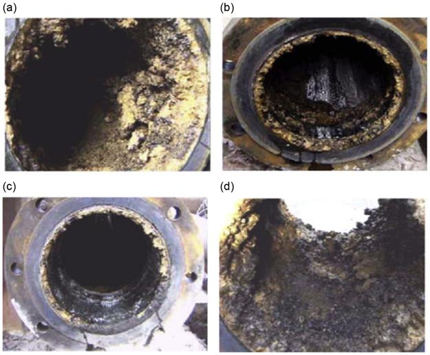
Nawrath et al. [1] performed an experimental study on a test rig with real Bayer liquor at Queensland Alumina Limited (QAL). They observed that the rate of scale growth is 60% higher in a concentric reducer than it is in adjacent pipes and the rate of scale growth is reduced to zero on the precipitator tank wall when slurry velocity is around 2.9 m s−1. Here, we present some practical examples of scale growth in pipe lines and fittings at QAL [1]. Figure 6.2(a) shows that the scale thickness in the downstream end of the concentric reducer of 350 mm diameter ranged between a maximum of 68 mm and a minimum of 26 mm; the deposit was a nodular, oxalate-containing gibbsite scale loosely bound. In Figure 6.2(c), scale growth at the discharge end of the 200 mm diameter pipe did not exceed 11 mm in thickness. In the 350×250 concentric reducer as shown in Figure 6.2(d), nodular oxalate crystals in the alumina hydrate scale resulted in characteristics of dark-colored scale.
6.3 Fundamentals of Scaling
Historically, interaction of particles with turbulent flow is characterized by the dimensionless particle relaxation time, which is the ratio of the particle relaxation time ![]() to the timescale of near-wall turbulent structures. The particle relaxation time [3] based on Stokes drag law is defined as:
to the timescale of near-wall turbulent structures. The particle relaxation time [3] based on Stokes drag law is defined as:
[6.1]
The Kolmogorov timescale of fluctuations based on volume-averaged viscous energy dissipation is [4]:
[6.2]
where ![]() is the friction velocity defined as:
is the friction velocity defined as:
[6.3]
where ![]() is the wall shear stress.
is the wall shear stress.
For a symmetrical developed pipe flow, when the wall shear stress at a pipe surface is uniform, the friction velocity may be expressed as a function of the average velocity and the friction factor f as:
[6.4]
The dimensionless particle relaxation time ![]() for a pipe flow yields from the combination of Eqs (6.1)– (6.4) as:
for a pipe flow yields from the combination of Eqs (6.1)– (6.4) as:
[6.5]
The behavior of the interaction of particles with turbulent flow is highly dependent on the value of their dimensionless relaxation time. If ![]() is very small, particles have the ability to closely follow all the turbulent fluctuations of a fluid [3]. At larger values of
is very small, particles have the ability to closely follow all the turbulent fluctuations of a fluid [3]. At larger values of ![]() , the trajectories of particles and their velocity deviate from the fluid particles’ path. Large particles are only slightly affected by small eddies, and respond mainly to the larger eddies which usually occur at greater distances from the wall [3].
, the trajectories of particles and their velocity deviate from the fluid particles’ path. Large particles are only slightly affected by small eddies, and respond mainly to the larger eddies which usually occur at greater distances from the wall [3].
6.4 Particle Deposition Mechanisms
In this section we discuss the physical processes by which solid particles suspended in a fluid are transported to, and deposited on, solid walls. Particle deposition is both significantly interesting and important in mechanical engineering, chemical engineering, environmental science, and medicine. Sippola and Nazaroff [5] summarized all forces and mechanisms influencing particle motion in turbulent flow. Brownian motion is present as a result of the random interaction between particles and fluid particles, given as:
[6.6]
where the Brownian diffusivity (![]() ) of a particle can be calculated by the Stokes–Einstein relation, which is defined as:
) of a particle can be calculated by the Stokes–Einstein relation, which is defined as:
[6.7]
Whenever there is relative motion between a particle and its surrounding air, the particle experiences a drag force from the air that tends to reduce that relative motion calculated as [5]:
(6.8)
If dispersed particles are denser than the fluid, they settle owing to the effects of gravitational acceleration, the net gravitational force on a particle is given by [5]:
[6.9]
A particle entrained in a shear flow field may experience a lift force perpendicular to the main stream flow direction. The magnitude of this shear lift force was first calculated by Saffman [6] as:
[6.10]
 [6.10]
Thermophoresis which is particle force resulting from temperature gradient is evaluated by balancing a drag force with the thermophoretic force, which acts in the direction of decreasing temperature, and is given by Talbot et al. [7] as:
[6.11]
where ![]() is the y-component of the temperature gradient and H is the thermophoretic force coefficient defined as:
is the y-component of the temperature gradient and H is the thermophoretic force coefficient defined as:
[6.12]
The turbulent fluctuations contribute to the diffusive flux of particles in the direction normal to the wall, defined as [5]:
[6.13]
where ![]() is the total diffusive flux and
is the total diffusive flux and ![]() is the contribution to the total diffusive flux from turbulent fluctuations.
is the contribution to the total diffusive flux from turbulent fluctuations.
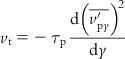
The dominant transport mechanism in turbulent flows near the wall due to the gradient in turbulent fluctuating velocity components gives rise to turbophoresis. Caporaloni et al. [8] were the first to recognize this phenomenon, and they calculated the turbophoretic velocity to be:
[6.14]
 [6.14]
Assuming that the drag force balances turbophoresis, the net turbophoretic force applied to a particle can be expressed as:
[6.15]
 [6.15]
Numerous reviews of turbulent particle deposition by Sippola and Nazaroff [5] have summarized most of the published experimental data on small vertical tubes. They have summarized the experimental data as represented in Figure 6.3 in the form of “dimensionless particle deposition velocity (![]() ) versus dimensionless particle relaxation time.” The “dimensionless particle deposition velocity (
) versus dimensionless particle relaxation time.” The “dimensionless particle deposition velocity (![]() )” is defined as:
)” is defined as:
[6.16]
where the average deposition velocity, ![]() , of a particle to a wall is given by [5]:
, of a particle to a wall is given by [5]:
[6.17]
where J is the time-averaged particle flux to the surface and ![]() is the time-averaged concentration of particles in the fluid. Since the data are presented in dimensionless form, they are applicable to any types of particle deposition from solution.
is the time-averaged concentration of particles in the fluid. Since the data are presented in dimensionless form, they are applicable to any types of particle deposition from solution.

Sippola and Nazaroff [5] have also summarized the experimental results into three different regimes as shown in Figure 6.3, these being the diffusion regime, the diffusion-impaction regime and the inertia-moderated regime.
In the diffusion regime, with ![]() , the dimensionless deposition velocity decreases as
, the dimensionless deposition velocity decreases as ![]() increases because of the decrease in Brownian diffusivity as particle size increases [5]. In this regime, particles are very small and they follow all turbulent eddies. When the no-slip condition of flow at the wall is fulfilled, they have less chance of touching the walls as the turbulent eddies do not penetrate through the laminar sublayer.
increases because of the decrease in Brownian diffusivity as particle size increases [5]. In this regime, particles are very small and they follow all turbulent eddies. When the no-slip condition of flow at the wall is fulfilled, they have less chance of touching the walls as the turbulent eddies do not penetrate through the laminar sublayer.
At the other end (inertia-moderated regime) of Figure 6.3, for the largest particle with ![]() , the dimensionless particle deposition velocity becomes almost constant and independent of particle size [5]. In an inertia-moderated regime, particles are too large to respond to the rapid fluctuations of near-wall eddies and transport to the wall by turbulent diffusion is very weak. These particles reach the wall through momentum imparted by large eddies in the core of the turbulent flow. This assumption agrees well with direct numerical simulation (DNS) modeling by Narayanan et al. [9], who found that the fraction of particles with
, the dimensionless particle deposition velocity becomes almost constant and independent of particle size [5]. In an inertia-moderated regime, particles are too large to respond to the rapid fluctuations of near-wall eddies and transport to the wall by turbulent diffusion is very weak. These particles reach the wall through momentum imparted by large eddies in the core of the turbulent flow. This assumption agrees well with direct numerical simulation (DNS) modeling by Narayanan et al. [9], who found that the fraction of particles with ![]() depositing in free-flight mode was around 40% and tends to increase with increasing
depositing in free-flight mode was around 40% and tends to increase with increasing ![]() .
.
In the diffusion-impaction regime, with ![]() , particle size increases and this provides more chance to deviate from the flow path of small eddies and to cross the laminar sublayer due to their inertia [5]. Aliseda et al. [10] experimentally investigated that, at
, particle size increases and this provides more chance to deviate from the flow path of small eddies and to cross the laminar sublayer due to their inertia [5]. Aliseda et al. [10] experimentally investigated that, at ![]() , particles show optimal sensitivity in absorbing kinetic energy from small eddies, which is combined with a sufficient ability of deviating from the fluid flow paths and of shooting across the laminar sublayer toward the wall. However, from these experiments, it is not fully understood as to why the dimensionless deposition velocity continued to increase up to the value of
, particles show optimal sensitivity in absorbing kinetic energy from small eddies, which is combined with a sufficient ability of deviating from the fluid flow paths and of shooting across the laminar sublayer toward the wall. However, from these experiments, it is not fully understood as to why the dimensionless deposition velocity continued to increase up to the value of ![]() . Many researchers [11] have assumed that this trend is associated with the increasing sensitivity of the particles to turbophoresis.
. Many researchers [11] have assumed that this trend is associated with the increasing sensitivity of the particles to turbophoresis.
Adomeit and Renz [12] presented both numerical and experimental work to investigate the transport mechanism, describing particle adhesion by the interaction forces. They found that transport is dominated by hydrodynamic lift and deposition of 1.2-µm particles is suppressed under laminar flow conditions. Matida et al. [13] numerically studied deposition of particles occurring toward the wall from a turbulent dispersed flow in a vertical pipe. They used a one-way coupling Lagrangian eddy–particle interaction model and found that the Saffman lift force had a considerable effect on deposition rate. Eskin et al. [14] studied a model of asphaltene deposition in a turbulent pipe flow which was examined by a Couette device. They observed that the precipitated particles grow due to agglomeration driven by the Brownian motion and turbulent dispersion.
Zonta et al. [15] numerically investigated the effect of swirl on near-wall turbulence and the mechanisms of particle separation by DNS and Lagrangian particle tracking. They observed that near-wall swirl flow increases the degree of drag due to higher-velocity wall-gradients and increases of wall shear stress due to transport of axial vorticity toward the radial periphery of the pipe. Greenfield and Quarini [16] numerically studied the effect of thermophoresis on the deposition of particles in a turbulent flow which is significant. They found that particles experience a force in the opposite direction to the temperature gradient and tend to deposit on cold walls and be repulsed by hot walls. Adomeit and Renz [12] presented numerically the effect of hydrodynamically induced lift on the deposition rate of particles from flowing suspensions to reduce the particle deposition rate and avoid surface contamination and fouling.
Zahmatkesh [17] studied numerically and showed that the dominant mechanism for deposition of ~100 µm particles was inertial impaction and deposition of ~10 µm particles was mainly influenced by thermophoresis. Yiantsios and Karabelas [18] experimentally investigated the deposition rates which were determined by optical microscopy and image analysis techniques. The authors observed that hydrodynamic wall shear stress increases particle deposition and hydrodynamic lift or drag forces inhibit transport or attachment. Zhao and Chen [19] described a numerical model and showed that the dimensionless deposition velocity becomes smaller due to Brownian diffusion and gets larger due to turbophoresis. They also concluded that, if particle diameter is smaller than 1 µm, the results with and without turbophoresis are nearly the same. Marchioli et al. [4] studied numerically connections among the turbulence structure of the boundary layer, particle transfer, and deposition mechanisms. They concluded that a particle was brought into the wall layer by a sweep and re-entrained to the outer flow by an ejection, and the particle may be trapped in the viscous region by the residual turbulence fluctuations of the viscous sublayer.
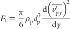
Soldati and Marchioli [11] summarized that particle deposition is a multi-step process: segregation, accumulation, and deposition as shown in Figure 6.4. In the first step, particles segregate and form coherent clusters in regions of the buffer layer. Then particles entrained in a sweep experience a net drift toward the near-wall accumulation region, where particle concentration reaches its maximum. In the practical investigation, the main mechanism capable of causing such drift is turbophoresis [4,9]. In the accumulation region, which is located well into the viscous sublayer, particles may either deposit at the wall or be re-entrained toward the flow by ejections. Two main deposition mechanisms can be identified [9,20]: particles that have acquired enough momentum may coast through the accumulation region and deposit by impaction directly at the wall. Otherwise, after a long residence time, particles can be deposited under the action of turbulent fluctuations.
6.5 Fluid Dynamics Analysis in Scale Growth and Suppression
Here, fundamentals of scale suppression mechanisms from the perspective of fluid dynamics are discussed. Very limited work has been done on scale formation mechanisms in slurry pipes and slurry tanks used in mineral-processing industries such as aluminum refineries. In the extensive literature, most of the topics are related to fouling in evaporators [21], membranes used in the reserve osmosis processes in desalination plants [22], and heat exchangers [23]. Loan et al. [24] in CSIRO (Commonwealth Scientific and Industrial Research Organisation), experimentally investigated scale formation in slurry tanks by X-ray photoelectron spectroscopy and they observed that, at the initial stage, scale is formed as a result of precipitation reactions other than solids settling. Many researchers [1,21,25,26] suggest that scale growth in the processing equipment is affected by a number of factors including supersaturation in solution, phase transformation, run time, form of material surfaces and flow characteristics (velocity, flow rate, and Reynolds number). In the chemical industry, slurry mixing tank agitators are often designed on the basis of achieving off-bottom suspension to resist the settle time for crystallization [27–29]. In this case, axial flow impellers pumping downward with vertical baffles are more energy-efficient than radial turbines [27–29] and the energy efficiency for off-bottom solids suspension is sensitive to impeller off-bottom clearance and impeller diameter [30–36].
A novel scale-velocity model was developed by Wu et al. [32] for explaining the scale growth and suppression in the precipitation regime an alumina refinery. In this model, a relationship between the fluid flow velocity and scale formation is schematically presented in Figure 6.5. There are four regimes identified to understand the scale growth mechanism, namely regimes (A) mass transfer control, (B) chemical reaction control, (C) suppression by erosion and (D) erosion damage. In regime A, the initial scale is null at zero velocity as followed by molecular diffusion-rate controlled process [32]. Then the scale growth rate starts very rapidly as fluid velocity increases due to an increased effect of mass transfer. This explanation is strongly supported by the study of Hoang et al. [25] into increase in gypsum scale growth rate with increasing fluid velocity in a range from 0 to 0.07 m s−1.
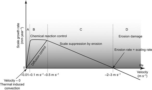
In regime B, for fluid velocity larger than 0.1 m s−1, the chemical reaction rate may start to control the overall rate of scaling as increasing fluid velocity does not affect the overall rate of scale growth [32]. On the other hand, when chemical reaction is relatively fast, the rate of scale growth continuously increases with increasing fluid velocity.
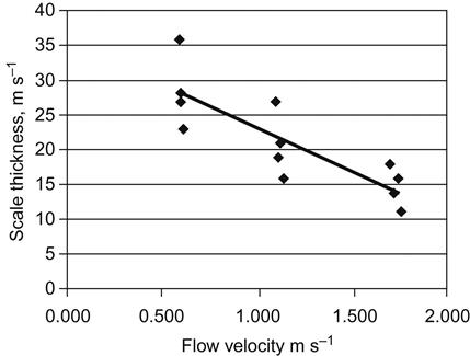
In regime C, the rate of scale growth gradually decreases with an increase in fluid velocity. In this regime, an increase in fluid velocity results in more erosion, which slows down the scale growth [32]. Nawrath et al. [1] conducted detailed plant tests on scale growth of a supersaturated aluminate solution in a precipitation circuit at a QAL refinery in Australia. Measurements of scale growth were conducted in a series of different diameter pipes connected through the fittings, and concluded that scale growth decreases with increasing slurry velocity in the range from 0.5 to 1.7 m s−1 as presented in Figure 6.6.
In regime D, the material surface suffers net loss due to the effect of erosion exceeding scale growth [32]. Wu et al. [34] reported on erosion of the impeller tip operating in a slurry vessel due to the increase in tip velocity of the blade as shown in Figure 6.7. The erosion increases with the increase in blade radius, due to increased tip velocity [32].

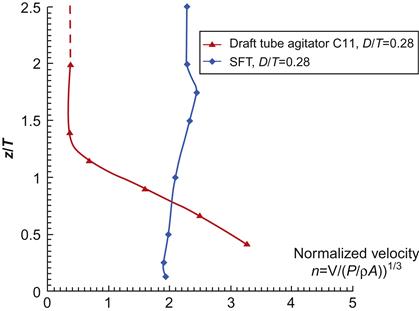
Wu et al. [32] concluded that regimes C and D are more important for scale suppression in terms of fluid dynamics design, and hydrodynamic lift and drag forces play a minor role in the nucleation of slurry particles to inhibit the scale growth. They invented a new precipitation tank design with swirl flow technology (SFT). It is the long-term experience that the velocity near the wall surface is a critical factor for suppression of scale growth [32]. The non-dimensional velocity efficiency parameter (![]() ) along the tank height can be described (Wu et al. [37]) by:
) along the tank height can be described (Wu et al. [37]) by:
[6.18]
where P is the agitator power input, ![]() is slurry density, A is the tank wetted surface area excluding the bottom and V is the velocity outside of the boundary layer.
is slurry density, A is the tank wetted surface area excluding the bottom and V is the velocity outside of the boundary layer.
From their experiment, Wu et al. [32] concluded that SFT creates a more uniform higher absolute velocity adjacent to the tank surface when compared with the conventional draft tube agitator design configurations as shown in Figure 6.8. For detailed investigation, CFD modelings were conducted on full-scale cone-bottom and flat-bottom precipitation tanks with the conventional draft-tube agitator and the swirl flow agitator (SFT). It was observed that the swirl flow agitator is more energy-efficient with the cone-bottom tank than the flat-bottom tank. Nawrath et al. [1] and Deev et al. [3] conducted extensive laboratory experiments to discern the effect of fluid dynamics of flow through the model of a concentric reducer used for connecting pipes of two different diameters. They measured the stream-wise and cross-stream velocity components of water flow through the concentric reducer by particle image velocimetry technology [3]. They found that the cross-stream component of the fluctuating velocity varies significantly and, at the distance from the wall of 0.05 R, the component becomes five times larger than that at the walls of the straight pipes connected to the reducer.
Hoang et al. [25] experimentally investigated the effects on gypsum scale formation in pipes of process parameters supersaturation ratio, run time, and operational hydrodynamic conditions (flow rate, fluid velocity, pipe diameter, and Reynolds number) and surface material. Cowan and Weintritt [38] conducted experiments with high-velocity flow which can curtail or accelerate scale deposition due to the formation of a boundary layer next to the pipe wall. Yu et al. [20] experimented with a dynamic system containing a fouling-loop in which the effects of thermodynamic conditions such as surface superheat, fluid velocity, and bulk subcooling on sugar mill evaporators were investigated. The fouling mechanism was particulate deposition of silica and calcium oxalate colloidal species, with the bond strength increased by consolidation; fouling rate increased with decreasing interfacial energy barrier between the heat exchange tube surface and foulant. Xiaokai et al. [26] experimentally determined that, at higher ion concentrations, the fouling rate increases linearly with surface temperature and the effect of flow velocity on deposition rate is very strong. It is clear that scaling is a physicochemical process which can be affected by fluid dynamics influences on heat and mass transfer. Therefore, fluid velocity plays a critical role in the scale suppression mechanism.
6.6 Target Model
Plant data indicate that the scale growth is significantly more in a concentric reducer than that in adjacent straight pipes contrary to conventional intuition. Nawrath et al. [1] experimentally observed that the rate of scale growth is 60% higher in a concentric reducer. It is important to elucidate the factors responsible for this higher scale deposition in the reducer. The full-scale concentric reducer was numerically modeled in this study as shown in Figure 6.9. The rate of contraction of the cross-sectional area of the reducer along its axis was not uniform. The rate of area reduction between sections A–A and B–B gradually increases and reaches its maximum rate near the section B–B as shown in Figure 6.10. This maximal reduction rate remained virtually constant throughout sections C–C and D–D, before gradually decreasing when approaching section E–E and then diminished to zero at section F–F. The rate of strain imposed on the flowing water could affect the behavior of the fluctuating velocity. The stream-wise (![]() ) and cross-stream (
) and cross-stream (![]() ) components of the instantaneous velocities were measured along several sections through: A–A to G–G as shown in Figure 6.10 [3]. Section A–A was positioned at the boundary between the end of the straight pipe and entrance to the reducer. The five sections B–B to F–F were separated from section A–A and from each other by the uniform distance of 15 mm. The last sections G–G and H–H were located within the smaller straight pipe at a distance of 36 and of 86 mm from F–F, respectively.
) components of the instantaneous velocities were measured along several sections through: A–A to G–G as shown in Figure 6.10 [3]. Section A–A was positioned at the boundary between the end of the straight pipe and entrance to the reducer. The five sections B–B to F–F were separated from section A–A and from each other by the uniform distance of 15 mm. The last sections G–G and H–H were located within the smaller straight pipe at a distance of 36 and of 86 mm from F–F, respectively.


Several researchers [39–45] have described the phenomenon of turbulent airflow through an axisymmetric contraction reducer. It was evident from those studies that the cross-stream fluctuating velocity components become dominant with the flow acceleration while passing through an axisymmetric contraction. A detailed experiment of the air flow in a gradually contracting pipe producing constant strain rate in a fluid has been carried out with 3D hot wire anemometry by Torbergsen and Krogstag [40]. It was found that, at a distance from the wall of about 60 dimensionless wall units, the stream-wise component (![]() ) experienced a threefold decrease, while the cross-stream component (
) experienced a threefold decrease, while the cross-stream component (![]() ) had a twofold increase for the flow through the contraction with a Reynolds number of 35,000, at the entry of contraction, and ratio of area contraction of 8. Tennekes and Lumley [46] presented a visual picture of how stream-wise vortex stretching increases the vortex angular velocity, thus suppressing stream-wise fluctuations (
) had a twofold increase for the flow through the contraction with a Reynolds number of 35,000, at the entry of contraction, and ratio of area contraction of 8. Tennekes and Lumley [46] presented a visual picture of how stream-wise vortex stretching increases the vortex angular velocity, thus suppressing stream-wise fluctuations (![]() ) in favor of cross-stream fluctuations (
) in favor of cross-stream fluctuations (![]() ).
).
6.7 Numerical Method
The governing equations being solved in Reynolds stress model (RSM) are continuity, momentum, and turbulence equations by commercial CFD code ANSYS fluent version 15.0. For an incompressible fluid, the equations of continuity and momentum balance for the mean motion are given as [47]:
[6.19]
[6.20]
where ![]() is the Reynolds stress tensor and
is the Reynolds stress tensor and ![]()
The RSM involves calculation of the individual turbulence stresses via a differential transport equation given as [47]:
[6.21]
 [6.21]
where the production is given as:
[6.22]
Here, ![]() ,
, ![]() and
and ![]() are empirical constants
are empirical constants ![]()
The turbulence dissipation rate ![]() is computed by the governing equation [47]:
is computed by the governing equation [47]:
[6.23]
The values of the constants are
The governing equations were discretized by using the vertex-centered finite volume method. The second-order central differencing scheme was applied for the spatial derivatives of the pressure term and the second-order upwind scheme was used for the momentum term. The specific dissipation rate and Reynolds stresses were discretized using the first-order upwind scheme. Pressure–velocity coupling was preserved by using the Coupled algorithm.
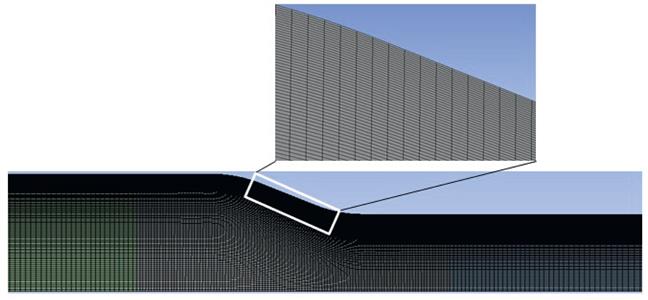
The preprocessor Design-Modeller was used to generate a two-dimensional Cartesian grid. The computational domain was discretized using quadrilateral structured meshes. Fine cells were used near the reducer wall, whereas coarser cells were adopted around the center of the reducer as shown in Figure 6.11. The mesh point distributions were concentrated near the reducer wall in order to give a more accurate boundary-layer solution. A turbulence intensity of 5% and a uniform velocity distribution ![]() (two values of 0.268 and 0.432 m s−1 considered) were defined at the inlet. All velocity components were gradient-free for the stream-wise direction at the outlet. Pseudo transient explicit relaxation factors of 0.5 for pressure, 0.5 for momentum, 1 for density, and 0.75 for specific dissipation rate were considered. The convergence criterion for all the parameters was set on the order of 10−5.
(two values of 0.268 and 0.432 m s−1 considered) were defined at the inlet. All velocity components were gradient-free for the stream-wise direction at the outlet. Pseudo transient explicit relaxation factors of 0.5 for pressure, 0.5 for momentum, 1 for density, and 0.75 for specific dissipation rate were considered. The convergence criterion for all the parameters was set on the order of 10−5.
6.8 Grid Independence Test
For the grid independence study, the working fluid has been taken as water and the simulation was run Re=27,130 and 43,740 based on an inlet diameter (D=101.8 mm) and two velocities (U0=0.268 and 0.432 m s−1, respectively). Grid independence testing was carried out to find out the optimum grid size for the numerical study.
Seven different grid sizes (250×80, 400×90, 600×110, 900×150, 1200×200, 1200×250, and 1200×270 termed Grid-1, Grid-2, Grid-3, Grid-4, Grid-5, Grid-6, and Grid-7, respectively) were tested to determine the effect on the pressure distribution calculated at section B (as shown in Figure 6.12) from the center to the wall. It was found that there was no significant change in pressure distribution beyond the grid size of 1200×250 (300,000 as Grid-6) which is shown in Figure 6.12. Therefore, for the numerical simulation, the grid size of 300,000 has been used to perform all the simulations.

6.9 Results and Discussion
6.9.1 Variation of Fluctuating Velocity Components along Radius
For each of the cross-sections A–A to G–G, the plots for the dimensionless root mean square (RMS) values of both stream-wise and cross-stream fluctuating velocity components (![]() and
and ![]() , respectively) were calculated as a function of the dimensionless distance from the wall in respect to the radius of the reducer (Y/R) at the two previously mentioned Reynolds numbers as shown in Figures 6.13–6.16. It has been found that the stream-wise (
, respectively) were calculated as a function of the dimensionless distance from the wall in respect to the radius of the reducer (Y/R) at the two previously mentioned Reynolds numbers as shown in Figures 6.13–6.16. It has been found that the stream-wise (![]() ) fluctuating velocity component (as shown in Figures 6.13 and 6.14) in the straight pipe section decreases about 1.5-fold than that in the reducer section and, in the core region, fluctuation almost vanishes. It is noteworthy that more fluctuation occurs in the reducer section than the straight pipe section and its influence on particle deposition rate.
) fluctuating velocity component (as shown in Figures 6.13 and 6.14) in the straight pipe section decreases about 1.5-fold than that in the reducer section and, in the core region, fluctuation almost vanishes. It is noteworthy that more fluctuation occurs in the reducer section than the straight pipe section and its influence on particle deposition rate.

 along the radius of the reducer: at the wall Y=R and Y/R=1, at the center Y=0 and Y/R=0. The data were measured at the four different cross-sections at Re=27,130.
 along the radius of the reducer: at the wall Y=R and Y/R=1, at the center Y=0 and Y/R=0. The data were measured at the four different cross-sections at Re=43,740.
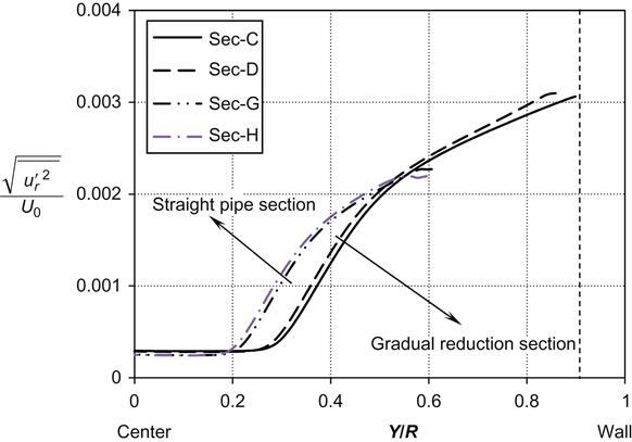
The variation of cross-stream (![]() ) fluctuating velocity components along the radius of the reducer was measured for both Reynolds numbers as shown in Figures 6.15 and 6.16. It has been found that the cross-stream (
) fluctuating velocity components along the radius of the reducer was measured for both Reynolds numbers as shown in Figures 6.15 and 6.16. It has been found that the cross-stream (![]() ) fluctuating velocity component in the core region almost vanishes. It is ascertained that the cross-stream fluctuating velocity component in the reducer section is higher than for the straight pipe section. In the reducer, the straining causes a severe reduction of the stream-wise fluctuating velocity component, and a similar gain in the cross-stream component, without changing the total kinetic energy.
) fluctuating velocity component in the core region almost vanishes. It is ascertained that the cross-stream fluctuating velocity component in the reducer section is higher than for the straight pipe section. In the reducer, the straining causes a severe reduction of the stream-wise fluctuating velocity component, and a similar gain in the cross-stream component, without changing the total kinetic energy.
6.9.2 Variation of Fluctuating Velocity Components Along Reducer Wall
The variations of both stream-wise (![]() ) and cross-stream (
) and cross-stream (![]() ) fluctuating velocity components along the reducer model were measured at a distance of 0.08 R from its wall. The results are presented in Figures 6.16 and 6.17 in the form of the RMS value of a respective fluctuating velocity component related to the mean in the 101.8 mm diameter pipe versus the distance from the section A–A measured along the axis of the reducer in the direction of flow.
) fluctuating velocity components along the reducer model were measured at a distance of 0.08 R from its wall. The results are presented in Figures 6.16 and 6.17 in the form of the RMS value of a respective fluctuating velocity component related to the mean in the 101.8 mm diameter pipe versus the distance from the section A–A measured along the axis of the reducer in the direction of flow.
 (
( ) and (
 ) along the X-axis at the distance of 0.08 R from the internal surface of the reducer: Re=27,130 and V=0.268 m s−1 (101.8 mmϕ pipe).
The stream-wise (![]() ) and cross-stream (
) and cross-stream (![]() ) fluctuating velocity components exhibit the following trends (as shown in Figure 6.17) as flow passes through the concentric reducer. For both Reynolds numbers, the stream-wise fluctuating component shows only a slight variation at the entry to the reducer, but it then increases more in the section between D–D to F–F. When the rate of contraction starts diminishing near the section F–F, the component
) fluctuating velocity components exhibit the following trends (as shown in Figure 6.17) as flow passes through the concentric reducer. For both Reynolds numbers, the stream-wise fluctuating component shows only a slight variation at the entry to the reducer, but it then increases more in the section between D–D to F–F. When the rate of contraction starts diminishing near the section F–F, the component ![]() shows a decrease for the inlet velocity of 0.268 m s−1 and a sharp decrease for the inlet velocity of 0.432 m s−1. The overall increase of
shows a decrease for the inlet velocity of 0.268 m s−1 and a sharp decrease for the inlet velocity of 0.432 m s−1. The overall increase of ![]() did not exceed 18% of its value at the entry to the reducer.
did not exceed 18% of its value at the entry to the reducer.
The cross-stream fluctuating velocity component ![]() reveals a remarkable increase between B–B to E–E and starts decreasing sharply after passing F–F. The cross-stream fluctuating velocity component
reveals a remarkable increase between B–B to E–E and starts decreasing sharply after passing F–F. The cross-stream fluctuating velocity component ![]() increases about twofold for the lower velocity and about 1.5-fold for the higher velocity (Figure 6.18).
increases about twofold for the lower velocity and about 1.5-fold for the higher velocity (Figure 6.18).
 () and () along the X-axis at the distance of 0.08 R from the internal surface of the reducer: Re=43,740 and V=0.432 m s−1 (101.8 mmϕ pipe).
As we discern from the theory, the value of the cross-stream fluctuating velocity component ![]() outside of the boundary layer is dominating parameters determining the deposition rate of particles suspended in the flowing fluid. The gradient of
outside of the boundary layer is dominating parameters determining the deposition rate of particles suspended in the flowing fluid. The gradient of ![]() pointing toward the solid surface determines both the rate of turbulent diffusion and the rate of turbophoresis for the particles depositing in the diffusion-impaction regime. It is ascertained that the increase in cross-stream fluctuating velocity component in the reducer has a strong influence to promote scale growth on the wall. In contrast, an increase in the stream-wise fluctuating velocity component is less pronounced but it accelerates the erosion of the deposited scale on the wall.
pointing toward the solid surface determines both the rate of turbulent diffusion and the rate of turbophoresis for the particles depositing in the diffusion-impaction regime. It is ascertained that the increase in cross-stream fluctuating velocity component in the reducer has a strong influence to promote scale growth on the wall. In contrast, an increase in the stream-wise fluctuating velocity component is less pronounced but it accelerates the erosion of the deposited scale on the wall.
6.9.3 Variation of Turbulent Kinetic Energy Along Radius
The variation of turbulent kinetic energy along the radius of the reducer was measured for both Reynolds numbers as shown in Figures 6.19 and 6.20. It has been found that the increase in turbulent kinetic energy is about threefold higher for the higher inlet velocity of 0.432 m s−1 than it is for the lower inlet velocity of 0.268 m s−1 in the reducer, and the level of turbulent kinetic energy remains constant in the core region. The variation in the turbulent kinetic energy supports the variation in the fluctuating velocity component.


6.10 Conclusions
This chapter dealt with particle deposition mechanisms and scale growth on solid walls of pipework in the Bayer process. A numerical study has been performed to assess the variation of fluctuating velocity components of water flow through the concentric reducer. According to the particle deposition theory in the diffusion-impaction regime, the cross-stream ![]() fluctuating velocity component is a dominant parameter controlling the variation of the particle deposition rate as flow passes through the reducer. The flow velocity of the fluid and the geometry of the pipe fittings affect the particle deposition rate. The cross-stream,
fluctuating velocity component is a dominant parameter controlling the variation of the particle deposition rate as flow passes through the reducer. The flow velocity of the fluid and the geometry of the pipe fittings affect the particle deposition rate. The cross-stream, ![]() fluctuating velocity component in the reducer is greater than the stream-wise
fluctuating velocity component in the reducer is greater than the stream-wise ![]() fluctuating velocity component in the reducer; it is believed that this is one of the reasons for more particle deposition as well as more scale growth in the concentric reducer. In contrast, the stream-wise
fluctuating velocity component in the reducer; it is believed that this is one of the reasons for more particle deposition as well as more scale growth in the concentric reducer. In contrast, the stream-wise ![]() fluctuating velocity component is responsible for erosion of deposited particles from the solid wall.
fluctuating velocity component is responsible for erosion of deposited particles from the solid wall.
Nomenclature
![]() Particle flux due to Brownian diffusion (kg m−2 s−1)
Particle flux due to Brownian diffusion (kg m−2 s−1)
![]() Brownian diffusion coefficient of a particle (m2 s−1)
Brownian diffusion coefficient of a particle (m2 s−1)
![]() Cunningham slip correction factor
Cunningham slip correction factor
![]() Drag force on a particle (kg m s−2)
Drag force on a particle (kg m s−2)
![]() Drag coefficient of spherical particle
Drag coefficient of spherical particle
![]() Gravitational force on a particle (kg m s−2)
Gravitational force on a particle (kg m s−2)
![]() Instantaneous stream-wise velocity (m s−1)
Instantaneous stream-wise velocity (m s−1)
![]() Thermopherotic force coefficient
Thermopherotic force coefficient
![]() Particle diffusive flux due to Brownian diffusion (kg m−2 s−1)
Particle diffusive flux due to Brownian diffusion (kg m−2 s−1)
![]() Fluctuating airborne particle concentration (kg m−3)
Fluctuating airborne particle concentration (kg m−3)
![]() Instantaneous local airborne particle concentration (kg m−3)
Instantaneous local airborne particle concentration (kg m−3)
![]() Dimensionless deposition velocity of particle to a wall
Dimensionless deposition velocity of particle to a wall
![]() Average deposition velocity of particles to wall (m s−1)
Average deposition velocity of particles to wall (m s−1)
![]() Time-average particle flux to the surface (kg m−2 s−1)
Time-average particle flux to the surface (kg m−2 s−1)
![]() Time-average concentration of particle in fluid (kg m−3)
Time-average concentration of particle in fluid (kg m−3)
![]() Mass eroded divided by the total mass of particle impinging on a material surface
Mass eroded divided by the total mass of particle impinging on a material surface
![]() Particle impinging velocity (m s−1)
Particle impinging velocity (m s−1)
![]() Cross-stream component of instantaneous velocity (m s−1)
Cross-stream component of instantaneous velocity (m s−1)
![]() Time-averaged value of the cross-stream velocity component (m s−1)
Time-averaged value of the cross-stream velocity component (m s−1)
![]() Fluctuating component of cross-stream velocity (m s−1)
Fluctuating component of cross-stream velocity (m s−1)
![]() Root-mean-square of the fluctuating cross-stream velocity
Root-mean-square of the fluctuating cross-stream velocity
![]() Stream-wise component of instantaneous velocity (m s−1)
Stream-wise component of instantaneous velocity (m s−1)
![]() Time-averaged value of the stream-wise velocity component (m s−1)
Time-averaged value of the stream-wise velocity component (m s−1)
![]() Fluctuating component of stream-wise velocity (m s−1)
Fluctuating component of stream-wise velocity (m s−1)
![]() Root-mean-square of the fluctuating stream-wise velocity
Root-mean-square of the fluctuating stream-wise velocity
Greek symbols
![]() Dimensionless particle relaxation time
Dimensionless particle relaxation time
![]() Lifetime of smallest eddies; Kolmogorov timescale of fluctuations based on the volume-averaged viscous energy dissipation (s)
Lifetime of smallest eddies; Kolmogorov timescale of fluctuations based on the volume-averaged viscous energy dissipation (s)
![]() Wall shear stress (kg m−1 s−2)
Wall shear stress (kg m−1 s−2)
![]() Kinematic viscosity of fluid (m2 s−1)
Kinematic viscosity of fluid (m2 s−1)
![]() Dynamic viscosity (kg m−1 s−1)
Dynamic viscosity (kg m−1 s−1)
![]() Particle velocity in axial direction (m s−1)
Particle velocity in axial direction (m s−1)
![]() Fluctuating wall normal velocity (m s−1)
Fluctuating wall normal velocity (m s−1)